Article

A Hybrid Geometric Morphometric Deep Learning Approach for Cut and Trampling Mark Classification

by
Lloyd A. Courtenay
1,2,3,*,
Rosa Huguet
2,3,4,
Diego González-Aguilera
1 and
José Yravedra
5,6
1
Department of Cartographic and Terrain Engineering, Higher Polytechnic School of Ávila, University of Salamanca, Hornos Caleros 50, 05003 Ávila, Spain
2
Área de Prehistoria, Universitat Rovira i Virgili (URV), Avignuda de Catalunya 35, 43002 Tarragona, Spain
3
Institut Català de Paleoecologia Humana i Evolució Social (IPHES), C/ Marcellí Domingo s/n, Campus Sescelades URV (Edifici W3) E3, 43700 Tarragona, Spain
4
Unit Associated to CSIC, Departamento de Paleobiologia, Museo de Ciencias Naturales, C/ José Gutiérrez Abascal, s/n, 28006 Madrid, Spain
5
Department of Prehistory, Complutense University, Prof. Aranguren s/n, 28040 Madrid, Spain
6
Director of the C. A. I. Archaeometry and Archaeological Analysis, Complutense University, Professor Aranguren s/n, 28040 Madrid, Spain
*
Author to whom correspondence should be addressed.
Appl. Sci. 2020, 10(1), 150; https://doi.org/10.3390/app10010150
Submission received: 28 October 2019 / Revised: 18 December 2019 / Accepted: 19 December 2019 / Published: 23 December 2019

Abstract

:

Featured Application

Cut mark identification and analysis is a fundamental component for archaeological investigation. Cut mark analysis, however, has been the root of great debates, with some authors claiming to have the oldest cut marks in or outside of Africa. If these marks were to truly be anthropic in nature, then the repercussions of these findings would produce a paradigm shift for our understanding of human evolution. Unfortunately, the majority of methods available for cut mark classification are namely qualitative in nature. Here we provide a new, highly powerful artificially intelligent neural network classification model that can be used to quantitatively and more objectively overcome these issues, using 3D digital microscopy, Deep Learning and Geometric Morphometrics to obtain up to 100% accuracy in some cases.

Abstract

The concept of equifinality is currently one of the largest issues in taphonomy, frequently leading analysts to erroneously interpret the formation and functionality of archaeological and paleontological sites. An example of this equifinality can be found in the differentiation between anthropic cut marks and other traces on bone produced by natural agents, such as that of sedimentary abrasion and trampling. These issues are a key component in the understanding of early human evolution, yet frequently rely on qualitative features for their identification. Unfortunately, qualitative data is commonly susceptible to subjectivity, producing insecurity in research through analyst experience. The present study intends to confront these issues through a hybrid methodological approach. Here, we combine Geometric Morphometric data, 3D digital microscopy, and Deep Learning Neural Networks to provide a means of empirically classifying taphonomic traces on bone. Results obtained are able to reach over 95% classification, providing a possible means of overcoming taphonomic equifinality in the archaeological and paleontological register.

Graphical Abstract

1. Introduction

The publication of the ‘oldest’ anthropic evidence of any type is always a problematic issue, usually drawing attention, criticism, and eventual debate on the quality of these findings from the entire archeological and paleontological community. Perfect examples of such debates can be observed in the claims of ~3.4 Ma cut marks from Dikika, Ehtiopia [1], which have since been heavily criticized and rejected [2,3]. Likewise, sites claiming to have ~2.6 Ma cut marks outside of Africa in the province of Quranwala, India [4], have drawn some speculation to their authenticity. In the Americas, ~130 ka anthropic bone breakage [5] are also noted to be located in areas with highly abrasive sediments and problematic taphonomic contexts. The current consensus for the oldest cut marks in Africa, however, remains to be those of Gona [6], dated to approximately between 2.1 and 2.58 Ma, while other promising results have been localized with 1.9 and 2.4 Ma in Northern Africa [7].
Taphonomic debates revolving around these topics are essential in understanding features of human evolution, considering how current theories argue meat-eating to be a fundamental component of our evolution [8,9,10,11]. The concept of butchery contains a multitude of different implications beginning with resource acquisition [8,12,13,14,15], as well as the cognitive technical capacities to manufacture the instruments used for such activities [16,17,18,19,20]. Dates of cut marks at 3.3 Ma implicate Australopithecine populations to be the first users of tools and butcherers in hominin pre-history [1], however authors are yet to come to an agreement as to whether these individuals were physically capable of such practices [16,17,18,19,20]. While an argument has been proposed to say that natural edges of unknapped stones could be used for butchery practices [1], other authors argue that experimentation is yet to be found that supports this claim [3]. Nevertheless, if these findings were to be real, then strong empirical evidence would be needed in support of such a hypothesis.
Recent advances in the development of new methodologies for the study of Bone Surface Modifications (BSMs) have been able to reveal interesting patterns in the in-depth study of taphonomic traces. The implementation of Geometric Morphometric studies has been able to reveal a means of inferring different tool use [21] as well as raw material management [21,22,23] through cut mark morphologies. Moreover, when applied to the carnivore induced BSMs, analysts have been able to differentiate between carnivore agents based on tooth mark morphologies [24,25,26,27]. The innovative introduction of Artificial Intelligence (AI) in taphonomy [26,27,28,29,30,31] has additionally been able to overcome multiple barriers imposed by subjectivity [32]. This presents a powerful tool for the construction of classification models, presenting a series of efficient tools for the processing of complex data.
Here we present the power of Feed Forward Neural Networks (FFNN) trained through Deep Learning (DL) for the processing of morphological data obtained with advanced 3D digital microscopy. These efforts attempt to overcome issues imposed by equifinality and subjectivity in taphonomic research, as well as complement previously obtained data regarding the effectivity of Machine Learning (ML) algorithms for the processing of Geometric Morphometric information [26]. Through this, we present a new means of classifying cut marks and trampling marks through their morphological attributes, as well as an empirically objective and quantitative approximation to their morphological description and characterization.

2. Materials and Methods

Experimental samples consisted of 80 cut marks and 251 trampling marks (Figure 1). Sample sizes where chosen in accordance with statistical power tests [33,34], defining a minimum sample size of 59 individuals as significant for the type of analysis performed within this paper (Cohen’s d = 0.52, α = 0.05, power = 0.8).
Cut marks (Figure 1A) were produced using simple flakes knapped by a single right-handed individual, experienced and familiar with lithic materials from the Olduvai Gorge and other Lower Pleistocene sites. The raw material used for these experiments was obtained directly from the Naibor Soit Inselberg of the Olduvai Gorge (Tanzania) [23]. This raw material consists of a coarse-grained quartzite frequently found in multiple sites of Beds I and II of the Olduvai Gorge. Cut marks were produced on a mixture of adult bovid and suid individuals on a number of different anatomical elements, including femora, tibiae, and humerii. All cut marks were produced by a single right-handed individual, perpendicular to the bone while the bone was fresh and the meat intact.
Trampling mark samples (Figure 1B) were obtained from Domínguez-Rodrigo et al. [36]’s sample. These traces were produced under a number of different experimental conditions. Experiments were carried out using cervid bones obtained from a legal organized hunting party. Anatomical elements present a mixture of axial and appendicular elements, including femora, tibiae, radii, ulnae, humerii, vertebrae, ribs, and scapulae. The majority of the meat from these bones were removed with metal knives, then sectioned into smaller pieces using an electric saw. Each bone was then examined to avoid misclassifying BSMs produced by the defleshing and sectioning processes. The sample was then separated into multiple subsamples that were subjected to different experimental conditions. The first variable considered was the sediment type. Five different sedimentary conditions were used, the first consisting in fine-grained sands (60–200 µm), followed by medium-grained sands (200–600 µm), coarse-grained sands (0.6–2 mm), a combination of the different sand types in a clay stratum, and finally gravels (>2 mm). Additional variables considered the time exposed to trampling (10 s or 2 min), the individuals producing the trampling (all students of varying weights), and whether the bones were dry or fresh when buried. For more details consult citation reference [36].

2.1. Digital Reconstruction Technique

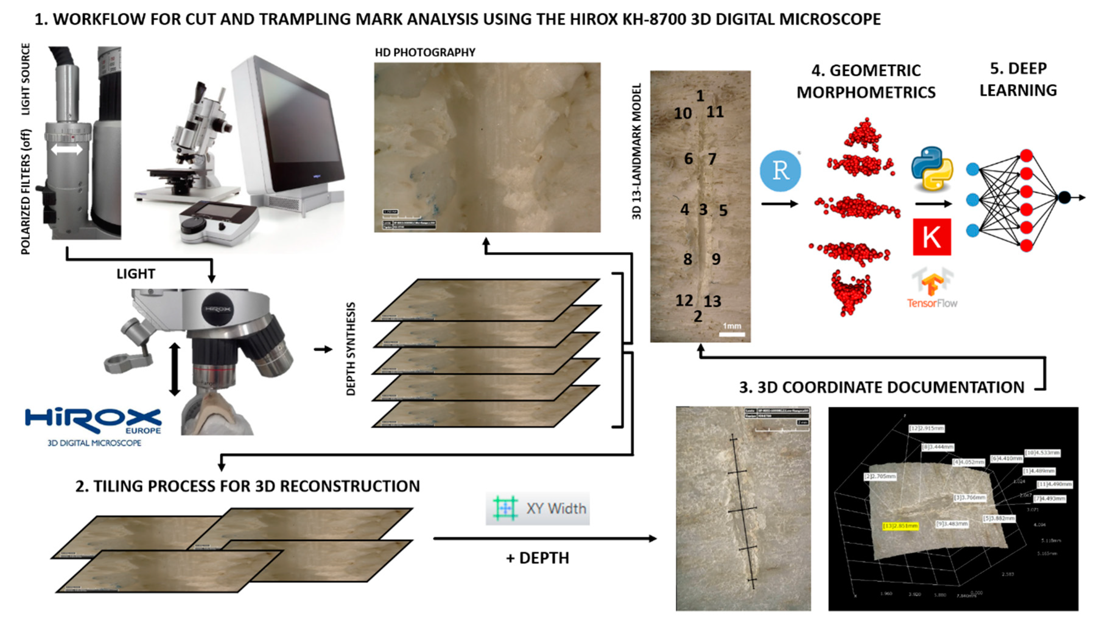
A combination of two different methodological approaches was used for this study, the first concerning the 3D digital reconstruction protocol via advanced digital microscopy [37] followed by the processing of this data via a 3D 13-landmark model [21].
The digitalization process was performed using the HIROX KH-8700 3D Digital Microscope with an MXG-5000 REZ triple objective revolving lens located in the Institut Català de Paleoecologia Humana I Evolució Social (IPHES), Tarragona, Spain. The HIROX is equipped with a high intensity LED light source that can be positioned around the subject of study. For this study, the light source was positioned directly above the object, combining both coaxial and ring lighting conditions without the use of any polarized filters. Digital reconstructions of each trace were performed between 100× (Field of View (FOV) = 1516 µm) and 200x (FOV = 3032 µm) magnification, using either the low or medium range lens. Three-dimensional reconstructions were produced using the HIROX’s mosaic tiling function, specifying a minimum of 30 photos per tile. This process takes approximately 13 min to complete per mark [37]. Collection of 3D landmark data was performed directly within the HIROX’s system software, employing the use of multiple measurement systems to obtain x, y, and z coordinates for the position of each landmark. This landmark data was then formatted and imported into R (https://www.r-project.org/) for further statistical analysis.
Further technical details regarding the microscope and a detailed description of the reconstruction protocol can be consulted in [37], as briefly and graphically described in Figure 2.

2.2. Geometric Morphometrics

Geometric morphometric analysis was performed in the free statistical software R (https://www.r-project.org/), employing the use of multiple packages that can be consulted in Appendix Table A1.
For the Geometric Morphometric analysis of both linear traces, a 3D 13-landmark model was used [21]. This model combines landmark types I and II to capture the internal as well as external morphological features of each trace. Landmark data is fist processed using a full Procrustes fit and an orthogonal tangent projection [38], known as Generalized Procrustes Analysis (GPA), normalizing data for further multivariate statistical analyses. GPA is a common practice in Geometric Morphometrics for the standardization of form information through multiple superimposition procedures, including translation, rotation, and scaling. Differences through this are revealed through patterns of variation and covariation that can be assessed statistically [39,40]. Principal Components Analyses (PCA) are performed on this data to reduce the complex combination of variables to fewer dimensions [39]. Additional thin plate splines, grid warpings, and mean shapes were calculated to visualize morphological variation across the Principal Component (PC) scores [39]. Degree of variance is then assessed using pairwise Multiple Variance Analyses (MANOVA). Depending on the inter-group homogeneity within each sample, MANOVA calculations were adjusted either using the Wilks or Hotelling–Lawley formula for inhomogeneous and homogeneous samples, respectively.
Samples were also processed using a Canonical Variance Analysis (CVA). CVA consists in the transformation of the raw PCA data, whereby pooled within-group dispersion are manipulated in a scaling process, thus standardizing within-group variance, and finally rotating the axes to be redrawn as a CVA graph [40]. Distances were then calculated between the groups with permutated p-values from the pooled within-group covariance matrices, calculating the degree of separation between samples in the form of Procrustes and Mahalanobis distances with their associated p-values of significance.
To ensure the efficiency of the learning process, PC scores were bootstrapped 1000× and extracted for the construction of Deep Learning Feed Forward Neural Network models.

2.3. Deep Learning

Deep Learning applications were programmed in Python (https://www.python.org/), using a number of different packages that can be consulted in Appendix Table A2. Algorithms conceptualized for supervised training and classification of samples consisted in the development of Feed Forward Neural Networks (FFNN). Neural Networks are modeled and coded to replicate brain patterns that are able to process highly complex and large sets of data [41], consisting of multiple nodes or perceptrons, which are connected by weighted axons or edges. These networks are designed to recognize patterns in order to interpret data, utilizing components of mathematics, calculus, linear algebra, and statistics to train and perform different tasks [42,43]. Likewise, this can be performed in a supervised, semisupervized, or unsupervised manner.
The FFNN designed for this study was constructed in TensorFlow 2.0 using the Keras API [41]. All Deep Learning implications were therefore run using TensorFlow as a backend engine on a portable laptop’s CPU (Intel® CoreTM i5 6300HQ), executed in a Conda (https://www.anaconda.com) virtual environment. The network was trained using the PC scores as dependencies, employing NumPy to convert PC scores into 64-bit floating point matrices. The associated class labels were indexed as separate 64-bit floating point vectors. PC scores are frequently used in Machine and Deep Learning as a method for projecting high-dimensional data into a new feature space that is useful for the training of AI models. Here we used the top 10 PC scores, representing 93% of the sample’s variance, using these PC scores to train models to classify unknown individuals.
A combination of neurons in a mixture of hidden layers are then used to map out the relationships between the dependency inputs (x) and the label outputs (y) [42,43]. A generalized mathematical representation of a single neuron can thus be represented as [42]:
y ( x ) = f ( i = 1 n w i x i )
where w are the weights connecting each neuron and f() represents an activation function that varies according to the position within the network [42]. Considering the case at hand consists in a binary classification problem, the label values were converted into a string of 1s and 0s indicating whether the taphonomic trace is anthropic (1) or not (0). In order to ensure that the model therefore only produces an output between 1 and 0, a sigmoid activation function is used for the final layer, described mathematically as [42]:
f ( x ) = 1 1 + e x
While all hidden layers were activated using the Rectified Linear Unit (ReLU) function [42]:
f ( x ) = max ( 0 , x )
During the learning process, the training of the model searches for the optimal combination of weights that can efficiently map out the y(x) relationship. Neural Networks are stochastic; therefore, weight initialization is performed at random [41,42,43,44]. The tuning of these weights was performed using back propagation and gradient descent via a stochastic optimization algorithm [42,43,45,46,47,48] and a binary cross entropy loss function [42,43].
For the purpose of configuring the neural network and finding the right hyperparameters during optimization, a series of trial runs were performed. These alternated between different combinations of hyperparameters, searching for the best results without overfitting. These trials employed typical practices of Deep Learning techniques [44], including changing the number of hidden layers, number of neurons per layer, batch size, epoch size, kernel constraints, weight regularization, the presence, position, or threshold of dropout layers as well as different optimization algorithms and learning rates. A summary of the hyperparameters tested can be consulted in Table 1.
Models were trained and evaluated using training, validation, and test splits. This is common practice in both Machine and Deep Learning [41,44,55]. The train-test split consisted of a 70:30% split ratio, respectively. During training, the training sample was further split using 30% for validation. FFNN were then trained on training and validation data, optimizing weights to improve the accuracy and reduce the loss. Learning curves were plotted to evaluate the increase/decrease of accuracy and loss over each iteration epoch. The metric used to evaluate the learning process while the model was being fit was set to ‘accuracy’. These learning curves could then be used to diagnose model behavior, thus evaluating whether the model was under- or overfitting on the training and validation data [44].
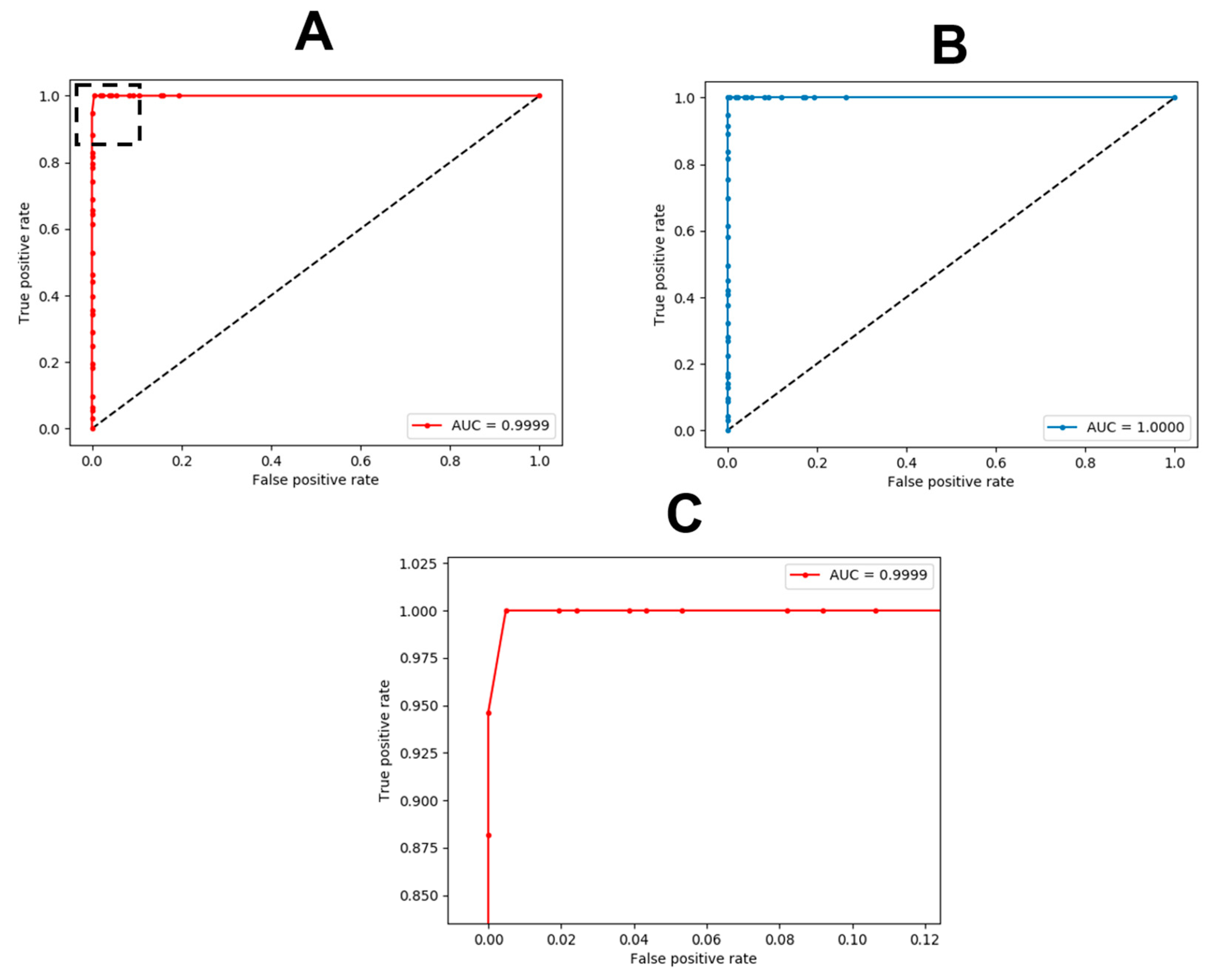
Final evaluation of the model was performed using the test set. The model was used to predict this ‘unknown’ data, recording both the accuracy and the loss obtained when predicting the missing label values from this data. The final metrics employed and evaluated using the test set consisted of sensitivity, specificity, and kappa values obtained via confusion matrices. The kappa (κ) statistic adjusts accuracy by considering the possibility of a correct prediction by change alone [55]. The resulting value is presented between −1 and 1, with a κ > 0.8 considered as a powerful predictive model. Sensitivity and specificity tests combine the frequencies and ratios of Type I and Type II statistical errors in proportion with the rest of the confusion matrix [56]. Values between 0 (poor) and 1 (high performing) indicate the predictive power of the model [55,56,57]. Further examination of the relationship between sensitivity and specificity in models was performed through the plotting of Receiver Operating Characteristic (ROC) curves and calculation of Area Under Curve (AUC) values [55,56]. ROC curves and AUC results are interpreted through the amount of space represented underneath the curve: the larger the area (AUC ≈ 1), the more accurate the model is when making predictions [55].
Considering the stochastic nature of FFNNs, evaluation and training was performed 30 times, taking averages of each numeric result to provide the final results. Results across all 30 iterations are provided as Tables S1 and S2. Confidence intervals were then calculated using the 2nd Standard Deviation (±2SD), thus representing approximately 95% of the deviation from the mean.
The final Python code used for this study is available in the form of a Jupyter Notebook online at https://github.com/LACourtenay/Deep-Neural-Network-for-Cut-Mark-Classification.

3. Results

3.1. Geometric Morphometrics

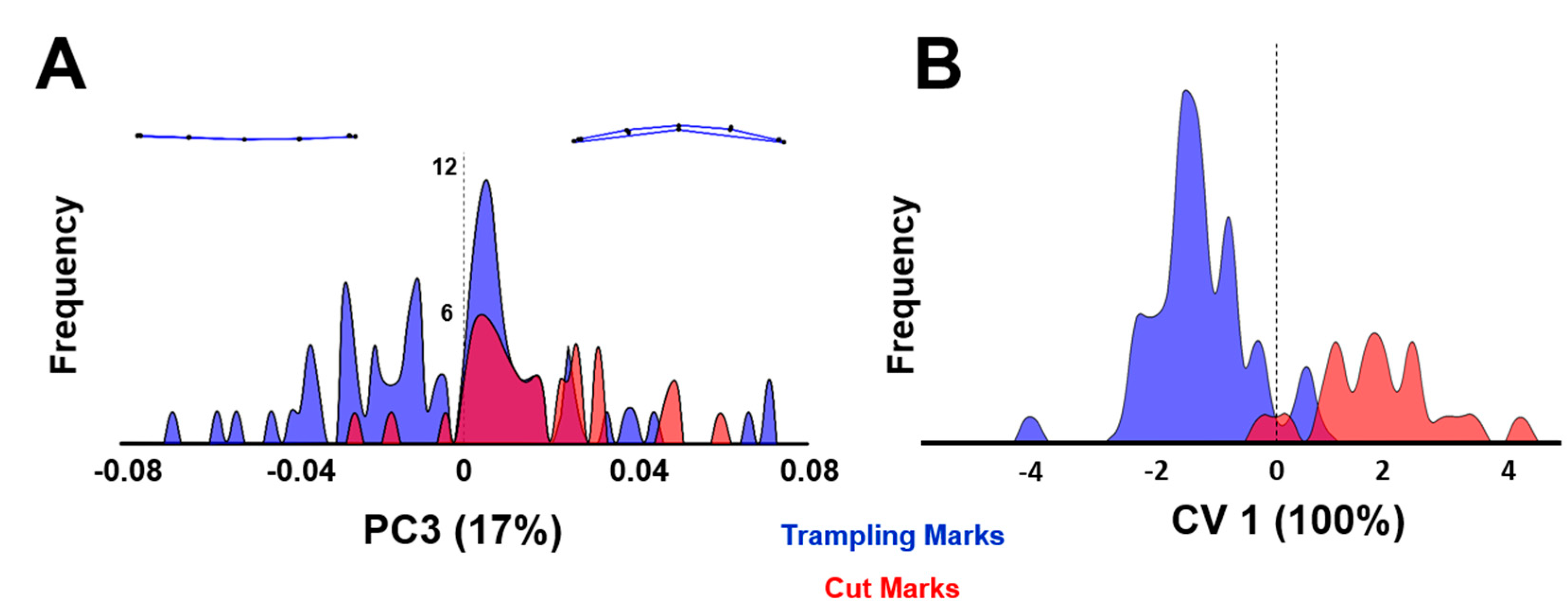
PCA was able to produce up to 32 PC scores, with the first 10 representing up to 93% of the total variance (Figure 3). The first two components of this analysis represent a cumulative variance of 52% of the sample, displaying a high degree of overlapping among trampling samples and anthropogenic cut marks. Regardless, trampling marks can be seen to represent a much greater degree of variability, with a much larger proportion of the sample displaying a trend toward a wider and more superficial morphology. Cut marks occupy a much smaller percentage of the overall feature space, leaning much closer to the end of PC1 that is represented by a finer groove. Additionally, trampling marks are also seen to vary greatly across the second principal component, which is represented by variations in groove trajectory. Contrarily, cut marks display a restricted distribution. Analysis of thin plate splines across PC3 displays a much clearer tendency for cut marks to lean toward deeper marks (Figure 4A), with trampling marks occupying primarily a percentage of feature space that is represented by very superficial traces.
Exploring these variations through numerical results highlight significant differences between samples, with MANOVA of p = 0.001 between both groups. Mahalanobis (D = 3.4403, p < 0.0001) and Procrustes (D = 0.0297, p = 0.0001) distance calculations also concur, with a clear separation between groups in CVA graphs (Figure 4B), represented by a total of 100% across the single axis of this figure.

3.2. Deep Learning

Initial trials prior to hyperparameter optimization and tuning began by achieving a model accuracy of approximately 70%, while overfitting proved to be a considerable issue with most model training and validation sets, even at this low degree of accuracy. After hyperparameter optimization, the final model obtained between 97.63% and 100% accuracy differentiating between trampling and cut marks (Figure 5, Table 2), presenting variation due to the stochastic nature of the model during weight initialization. The final model employed the use of 6 layers, 5 standard neural layers, and 1 dropout layer (Figure 5A and Figure S1). The inclusion of a larger density layer after the input (number of neurons = 20) produced a significant boost in accuracy, yet in order to prevent this additional layer from producing an over generalization of the data, a dropout layer with a constraint threshold of 0.5 was included directly afterwards (Figure 5A and Figure S1). A number of different positions for the dropout layer were tried and tested, yet the best results were obtained positioning said dropout in-between layers 3 and 5. An additional “UnitNorm” weight constraint was used to reduce overfitting, while the best training performance was obtained using the Adam optimization algorithm (learning rate (α) = 0.001, decay (β1) = 0.9). No additional regularization or kernel initialization techniques were found necessary for the final model.
The final training process used 900 epochs and a microbatch size of 64, obtaining an average accuracy of 99.55 ± 1.32% across training, testing, and validation samples (Figure 5B, Table 2 & Table S1). Loss on all accounts highlights the FFNN to be a powerful classifier with high confidence when assigning class labels to new individuals (Figure 5C). In training the average loss was recorded at 0.05, while 0.02 was recorded for validation and 0.01 for testing (Table 2, Table S1).
Further model evaluation through confusion matrices obtained on model testing was able to confirm the FFNN to be a highly efficient classification model, differentiating between cut and trampling marks with κ values of 1 ± 0.008 (Table 3, Table S2). Likewise, both sensitivity and specificity values averaged at 1 with the lowest specificity value being recorded at 0.995 and all sensitivity values obtaining 1 as well (Figure 6, Table 3, Table S2). ROC graphs almost always display a perfect right hand angle rather than a curve (Figure 6), with AUC values averaging at 1 ± 1.2 x 10⁻⁴.
Finally, FFNN training time averaged at 10.87 s while taking as little as ~17 milliseconds when making predictions.

4. Discussion and Conclusions

BSM analysis remains to be a very important component of taphonomic studies, whereby their identification and in-depth analysis can reveal multiple components regarding early hominin populations [11,12,13,14,15], their development [6,7,23], and their associated paleoecologies [14,24,28]. Nevertheless, issues imposed by equifinality have led to complications in their identification and interpretation [1,2,3,4,5], requiring more objective and empirical methods that can be used for BSM classification and characterization [21,22,23,24,25,26,27,30,58].
In recent years, debates regarding the protocol used to identify cut marks have ranged from simple observational criteria [58] to developments with a more complex multivariate protocol [36] and advanced microscopic studies [59]. With the integration of ML to the processing of qualitative data, analysts have been able to improve the processing of archaeological data sets to a considerable degree [29]; nevertheless, the subjective nature upon which this data is obtained makes some of these advances debatable [32]. One alternative has been proposed utilizing DL convolutional neural network architectures for image processing and classification [30], presenting promising results for automated BSM identification. Here, we additionally present the combined usage of advanced digital microscopy, Geometric Morphometrics, and artificially intelligent computational algorithms for cut mark identification and characterization. On both accounts, ML and DL have effectively proven to outperform human performance [29,30,32], presenting a more objective and precise means of studying microscopic traces.
The present results are able to develop data observed by multiple authors [12,36,37,58], yet employing new empirical means of quantifying these conclusions. Geometric morphometric characterization of trampling and cut marks concur that the most significant features of cut marks are their depth and straight trajectory, while trampling marks are more variable presenting much more superficial morphologies alongside other irregularities [37]. Furthermore, the ability of high-resolution 3D digital microscopy to overcome limitations imposed by the superficial nature of some traces [37] can also be considered a significant improvement from previous efforts [21,22]. While equifinality can still be observed to a certain degree, considering the high degree of overlap in most of these samples, it is important to point out the high dimensionality of PCA results derived from morphological data, as seen in how MANOVA testing is still able to identify significant differences between samples. Moreover, FFNN efficiently differentiates experimental samples with high levels of confidence on all accounts, considering their ability to extract complex patterns from difficult data [60].
The present study additionally complements previous efforts to implement ML algorithms in Geometric Morphometric analyses, expanding the available toolbox for morphological studies [26,61,62,63,64,65,66]. Courtenay et al. [26]’s original attempts to implement neural network architectures for tooth mark classification performed poorly, attributed by the authors to the model’s superficial nature. The complexity of the model here supports this observation. These results thus confirm model configuration and tuning to be essential for efficient classification, requiring extensive experimentation to find the optimal model. This would also explain the mixed results obtained by similarly superficial models in applications for systematic biology [61,62,63,64,65,66].
The field of AI can be seen to have exponentially grown since its conceptualization, providing algorithmic computational means of processing complex data sets. Many of these algorithms have presented significant advances for other disciplines, including medical research [67], pharmaceutics [68], business studies [69], engineering [70], and any other fields that require the advanced processing of large and complex data sets [60]. In prehistoric archaeology, ML and DL have arrived relatively late, yet present promising results. Nevertheless, problems of true experimental analogy are needed before these approaches can be applied on a broader scale. Here, Naibor Soit quartzite is used, considering this raw material’s importance in many Pleistocene sites of the Olduvai Gorge; however, if this approach were to be applied to other sites in Europe, Asia, or the Americas, then the experimental protocol and reference sample should be adjusted accordingly. Moreover, analysts should be aware of the possible overlapping traces that may increase the effects of taphonomic equifinality over time, such as fluvial abrasion, chemical alterations, and general loss of cortical surfaces [71,72], to name a few.
In other practical cases, the drawbacks of DL can be presented by limited sample sizes as well as the cost of training. This is especially apparent in archaeology and palaeoanthropology considering the conservation and preservation of the fossil record present considerable limitations. Nevertheless, Geometric Morphometric data has still proven to be a powerful type of input data for training, proving relatively fast to learn patterns from >1 min. Furthermore, considering the nature of the landmark data involved and its consequent transformation through GPA and PCA dimensionality reduction methods, this type of input data is less prone to issues presented by sample size as opposed to studies concerning, for example, Computer Vision and image processing-based techniques [54,73,74,75,76], the latter requiring large amounts of parameters (usually in the millions), which are hard to learn from small datasets [76].
Needless to say, as with the case of any innovative methodological introduction in archaeological and paleontological research, a large-scale use of these techniques is usually slow and requires large experimental programs to truly fine tune these results and examine their limitations.
DL and ML provide a significant advance for classification problems and predictive modeling [55], almost regardless of the type of data being analyzed. Advances in data science are presenting new means of automating data collection and processing, presenting a new empirical basis that can be used to confirm or reject cases of controversial taphonomic interpretations [1,4,5]. Neural Networks are highly versatile computational algorithms and can be adapted to most data sets [41,60]. Their success, however, is highly dependent on the tuning of their configuration and the developments available when considering the options feature engineering and hyperparameter optimization may provide [44,54,60,75,76]. Here, we have tested the potential of Deep Learning on the processing of morphological data to provide a hybrid approach that efficiently overcomes one of the taphonomy’s biggest questions. The present work thus demonstrates an example of how advanced microscopy and developed artificially intelligent algorithms may provide a promising future for archaeological and paleontological science.

Supplementary Materials

The following are available online at https://www.mdpi.com/2076-3417/10/1/150/s1: Figure S1: Visualization of the Neural Network Architecture. Bias neurons are represented in green, hidden neurons in blue and the dropout layer in red., Table S1: Accuracy and Loss Results from 30 prediction iterations on training, validation and test data, and Table S2: Results from 30 prediction iterations on test data.

Author Contributions

Conceptualization, L.A.C., R.H., and J.Y.; methodology, L.A.C.; software, L.A.C.; validation, L.A.C.; formal analysis, L.A.C.; investigation, L.A.C.; resources, L.A.C., R.H., and J.Y.; data curation, L.A.C.; writing—original draft preparation, L.A.C.; writing—review and editing, L.A.C., R.H., D.G.-A., and J.Y.; visualization, L.A.C.; supervision, R.H. and J.Y.; project administration, R.H., D.G.-A., and J.Y.; funding acquisition, R.H. and D.G.-A. All authors have read and agreed to the published version of the manuscript.

Funding

This research received no external funding.

Acknowledgments

First we would like to thank Manuel Domínguez-Rodrigo for providing the experimental samples used within this study. We would also like to acknowledge his inspirational work in this field. We would like to thank all the staff and members of both the IPHES and the Rovira I Virgili Univeristy. The corresponding author would also like to acknowledge the support provided by the TIDOP Groups 1 & 2 from the Department of Cartographic and Land Engineering of the Higher Polytechnics School of Avial, University of Salamance, and especially the help, advice, and support provided by Diego González-Aguilera and Miguel Ángel Maté-González. We would also like to thank Andreu Ollé for his advice, support, and interest in this research, as well as his technical support regarding the microscope and the lithic implements used within this study. We would also like to thank the helpful comments and suggestions provided by two anonymous reviewers and the editorial staff of MDPI. Finally, this work was supported by MICINN-FEDER PGC2018-093925-B-C32 and the AGUAR project number SGR 2017-1040: the Universitat Rovira I Virgili (2014, 2015, and 2016 PFR-URV-B2-17).

Conflicts of Interest

The authors declare no conflicts of interest.

Appendix A

For the purpose of this study, a mixture of R (https://www.r-project.org/) (Table A1) and Python (https://www.python.org/) (Table A2) were used for data science applications.
Table A1. Table presenting the R libraries used for geometric morphometric applications.
LibraryUsed For:Link
GeomorphGeneralized Procrustes Analysis
Principal Components Analysis
Thin Plate Splines
https://cran.r-project.org/web/packages/geomorph/geomorph.pdf
ShapesCanonical Variate Analysishttps://cran.r-project.org/web/packages/shapes/shapes.pdf
RVAideMemoireMultivariate Variance Analysishttps://cran.r-project.org/web/packages/RVAideMemoire/RVAideMemoire.pdf
Table A2. Table presenting the Python libraries used for Deep Learning applications.
LibraryUsed for:Link
TensorFlow 2.0.
Keras API
Neural Network Construction
Hyperparameter Optimization
https://www.tensorflow.org/
https://keras.io/
NumpyNumerical applications and operations
Slicing, indexing and transformation of data
https://www.numpy.org/
PandasLoading datahttps://pandas.pydata.org/
MatplotlibPlotting learning curves and ROC resultshttps://matplotlib.org/
Scikit-LearnModel evaluationhttps://scikit-learn.org/
For handling of Python and Deep Learning applications, the open source Anaconda (https://www.anaconda.com/) software was used to manage libraries and internal environments for Deep Learning. For debugging of Python code Jupyter Notebook (https://jupyter.org/) was used. For debugging of R code, R-Studio was used (https://www.rstudio.com/).

References

  1. McPherron, S.P.; Alemseged, Z.; Marean, C.W.; Wynn, J.G.; Reed, D.; Geraads, D.; Bobe, R.; Béarat, H. Evidence for stone-tool-assisted consuption of animal tissues before 3.39 million years ago at Dikika, Ethiopia. Nat. Lett. 2010, 466, 857–860. [Google Scholar] [CrossRef]
  2. Domínguez-Rodrigo, M.; Pickering, T.R.; Bunn, H.T. Experimental study of cut marks made with rocks unmodified by human flaking and its bearing on claims of ~3.4-Million-Year-Old butchery evidence from Dikika. J. Arch. Sci. 2012, 39, 205–214. [Google Scholar] [CrossRef]
  3. Domínguez-Rodrigo, M.; Alcalá, L. 3.3 million year old stone tools and butchery traces? More evidence needed. Paleoanthropology. 2016, 2016, 46–53. [Google Scholar]
  4. Malassé, A.D.; Moigne, A.M.; Singh, M.; Calligaro, T.; Karir, B.; Gaillard, C.; Kaur, A.; Bharwaj, V.; Pal, S.; Abdessadok, S.; et al. Intentional cut marks on bovid from the Quranwala Zone, 2.6 Ma, Siwalik Frontal Range, Northwestern India. Comptes Rendus Palevol 2016, 15, 317–339. [Google Scholar] [CrossRef] [Green Version]
  5. Holen, S.R.; Deméré, T.A.; Fisher, D.C.; Fullagar, R.; Paces, J.B.; Jefferson, G.T.; Beeton, J.M.; Cerutti, R.A.; Rountret, A.N.; Vescera, L.; et al. A 130,000 year old archaeological site in Southern California, USA. Nature 2017, 544, 479–483. [Google Scholar] [CrossRef] [PubMed]
  6. Domínguez-Rodrigo, M.; Pickering, T.R.; Semaw, S.; Rogers, M.J. Cutmarked bones from Pliocene archaeological sites at Gona, Afar, Ethiopia: Implications for function of the world’s oldest stone tools. J. Hum. Evol. 2005, 48, 109–121. [Google Scholar] [CrossRef] [PubMed]
  7. Sahnouni, M.; Parés, J.M.; Duval, M.; Cáceres, I.; Harichane, Z.; van der Made, J.; Pérez-González, A.; Abdessadok, S.; Kandi, N.; Derradji, A.; et al. 1.9-Million-Year and 2.4-Million-Year-Old Artifacts and Stone Tool-Cutmarked bones from Ain Boucherit, Algeria. Science 2019, 362, 1297–1301. [Google Scholar] [CrossRef] [PubMed] [Green Version]
  8. Bunn, H.T. Meat Eating and Human Evolution: Studies on the Diet and Subsistence Patterns of Plio-Pleistocene Hominids in East Africa. Ph.D. Thesis, University of California, Oakland, CA, USA, 1982. [Google Scholar]
  9. Milton, K. Primate Diets and Gut Morphology: Implications for Hominid Evolution. In Food and Evolution: Toward a Theory of Human Food Habits; Harris, M., Ross, E.B., Eds.; Temple University: Philadelphia, PA, USA, 1987; pp. 93–115. [Google Scholar]
  10. Aiello, L.C.; Wheeler, P. The expensive tissue hypothesis. Curr. Anthropol. 1995, 36, 199–221. [Google Scholar] [CrossRef]
  11. Stanford, C.B.; Bunn, H.T. Meat Eating and Human Evolution; Oxford University: Oxford, UK, 2001. [Google Scholar]
  12. Binford, L.R. Bones: Ancient Men and Modern Myths; Academic Press: New York, NY, USA, 1981. [Google Scholar]
  13. Blumenschine, R. Percussion marks, tooth marks and experimental determinations of hominid and carnivore access to long bones at FLK Zinjanthropus, Olduvai Gorge, Tanzania. J. Hum. Evol. 1995, 29, 21–51. [Google Scholar] [CrossRef]
  14. Domínguez-Rodrigo, M. Meat-eating by early hominids at the FLK-22 Zinjanthropus Site, Olduvai Gorge, Tanzania: An experimental approach using cut mark data. J. Hum. Evol. 1997, 33, 669–690. [Google Scholar] [CrossRef]
  15. Domínguez-Rodrigo, M.; Barba, R. New estimates of tooth mark and percussion mark frequencies at the FLK-Zinj Site: The carnivore-hominid-carnivore hypothesis falsified. J. Hum. Evol. 2006, 50, 170–194. [Google Scholar] [CrossRef] [PubMed]
  16. Toth, N.; Schick, K. The Oldowan: Case Studies into the Earliest Stone Age; Stone Age Institute Press: Gosport, England, 2006. [Google Scholar]
  17. Key, A.J.M.; Dunmore, C.J. The evolution of the Hominin thumb and the influence exerted by non-dominant hand during stone tool production. J. Hum. Evol. 2015, 78, 60–69. [Google Scholar] [CrossRef] [PubMed]
  18. Toth, N.; Schick, K. An Overview of the Cognitive Implications of the Oldowan Industrial Complex. Azania Arch. Res. Afr. 2018, 53, 3–39. [Google Scholar] [CrossRef] [Green Version]
  19. Semaw, S.; Roberts, M.J.; Quade, J.; Renne, P.R.; Butler, R.F.; DOmínguez-Rodrigo, M.; Stout, D.; Hart, W.S.; Pickering, T.; Simpson, S.W. 2.6 million year old stone tools and associated bones from OGS-6 and OGS-7, Gona, Afar, Ethiopia. J. Hum. Evol. 2003, 45, 169–177. [Google Scholar] [CrossRef]
  20. Domalain, M.; Bertin, A.; Daver, G. Was Australopithecus Afarensis able to make the Lomekwian Stone Tools? Towards a realistic biomechanical simulation of hand force capability in fossil hominins and new insights on the role of the fifth digit. Comptes Rendus Palevol 2017, 16, 572–584. [Google Scholar] [CrossRef] [Green Version]
  21. Courtenay, L.A.; Yravedra, J.; Maté-González, M.Á.; Aramendi, J.; González-Aguilera, D. 3D analysis of cut marks using a new geometric morphometric methodological approach. J. Arch. Anthr. Sci. 2019, 11, 651–665. [Google Scholar] [CrossRef]
  22. Maté-González, M.Á.; Palomeque-González, J.F.; Yravedra, J.; González-Aguilera, D.; Domínguez-Rodrigo, M. Micro-photogrammetric and morphometric differentiation of cut marks on bones using metal knives, quartzite and flint flakes. J. Arch. Anthr. Sci. 2016, 10, 805–816. [Google Scholar] [CrossRef]
  23. Courtenay, L.A.; Yravedra, J.; Aramendi, J.; Maté-González, M.Á.; Martín-Perea, D.M.; Uribelarrea, D.; Baquedano, E.; González-Aguilera, D.; Domínguez-Rodrigo, M. Cut marks and raw material exploitation in the Lower Pleistocene Site of Bell’s Korongo (BK, Olduvai Gorge, Tanzania): A geometric morphometric analysis. Quat. Int. 2019, 526, 155–168. [Google Scholar] [CrossRef]
  24. Aramendi, J.; Maté-González, M.A.; Yravedra, J.; Cruz Ortega, M.; Arriaza, M.C.; González-Aguilera, D.; Baquedano, E.; Domínguez-Rodrigo, M. Discerning carnivore agency through the three-dimensional study of tooth pits: Revisiting crocodile feeding leistoc at FLK-Zinj and FLK NN3 (Olduvai Gorge, Tanzania). Palaeogeog. Palaeoclimat., Palaeoecol. 2017, 488, 93–102. [Google Scholar] [CrossRef]
  25. Yravedra, J.; García Vargas, E.; Maté González, M.A.; Aramendi, J.; Palomeque-González, J.; Vallés-Iriso, J.; Matasanz-Vicente, J.; González-Aguilera, D.; Domínguez-Rodrigo, M. The use of micro-photogrammetry and geometric morphometrics for identifying carnivore agency in bone assemblage. J. Arch. Sci. Rep. 2017, 14, 106–115. [Google Scholar] [CrossRef]
  26. Courtenay, L.A.; Yravedra, J.; Huguet, R.; Aramendi, J.; Maté-González, M.Á.; González-Aguilera, D.; Arriaza, M.C. Combining Machine Learning Algorithms and Geometric Morphometrics: A Study of Carnivore Tooth Marks. Palaeogeo Palaeoclim. Palaeoecol. 2019, 522, 28–29. [Google Scholar] [CrossRef]
  27. Yravedra, J.; Maté-González, M.Á.; Courtenay, L.A.; González-Aguilera, D.; Fernández Fernández, M. The use of canid tooth marks on bone for the identification of livestock predation. Sci. Rep. 2019, 9, 16301. [Google Scholar] [CrossRef] [PubMed] [Green Version]
  28. Arriaza, M.C.; Domínguez-Rodrigo, M. When Felids and Hominins ruled at Olduvai Gorge: A Machine Learning Analysis of Skeletal Profiles of the Non-Anthropogenic Bed I Sites. Quat. Sci. Rev. 2016, 139, 43–52. [Google Scholar] [CrossRef]
  29. Domínguez-Rodrigo, M. Successful classification of experimental Bone Surface Modifications (BSM) through Machine Learning algorithms: A solution to the controversial use of BSM in paleoanthropology? J. Arch. Anthro. Sci. 2019, 11, 2711–2725. [Google Scholar] [CrossRef]
  30. Byeon, W.; Domínguez-Rodrigo, M.; Arampatzis, G.; Baquedano, E.; Yravedra, J.; Maté-González, M.A.; Koumoutsakos, P. Automated identification and deep classification of cut marks on bones and its palaeoanthropological implications. J. Comp. Sci. 2019, 32, 36–43. [Google Scholar] [CrossRef]
  31. Moclán, A.; Domínguez-Rodrigo, M.; Yravedra, J. Classifying agency in bone breakage: An experimental analysis of fracture planes to differentiate between hominin and carnivore dynamic and static loading using machine learning (ML) algorithms. Archae. Anthro. Sci. 2019, 11, 4463–4680. [Google Scholar] [CrossRef]
  32. Domínguez-Rodrigo, M.; Saladié, P.; Cáceres, I.; Huguet, R.; Yravedra, J.; Rodríguez-Hidalgo, A.; Martín, R.; Pineda, A.; Marín, J.; Gené, C.; et al. use and abuse of cut mark analyses: The Rorschach Effect. J. Arch. Sci. 2017, 86, 14–23. [Google Scholar] [CrossRef]
  33. Domínguez-Rodrigo, M.; Juana, S.; Galán, A.B.; Rodríguez, M. A New Protocol to Differentiate Trampling Marks from Butchery Marks. J. Archaeol. Sci. 2009, 36, 2643–2654. [Google Scholar] [CrossRef]
  34. Cohen, J. Statistical Power Analysis for Behavioural Sciences; Lawrence Erlbaum Assoc.: Mahwah, NJ, USA, 1988. [Google Scholar]
  35. Courtenay, L.A.; Maté-González, M.Á.; Aramendi, J.; Yravedra, J.; González-Aguilera, D.; Domínguez-Rodrigo, M. Testing Accuracy in 2D and 3D Geometric Morphometric methods for cut mark identification and classification. PeerJ 2018, 6, e5133. [Google Scholar] [CrossRef] [Green Version]
  36. Yravedra, J.; Diez-Martín, F.; Egeland, C.P.; Maté-González, M.Á.; Palomeque-González, J.F.; Arriaza, M.C.; Aramendi, J.; García Vargas, E.; Estaca-Gómez, V.; Sánchez, P.; et al. FLK-West (Lower Bed II, Olduvai Gorge, Tanzania): A newearly Acheulean site with evidence for human exploitation of fauna. Boreas 2017, 46, 486–502. [Google Scholar] [CrossRef]
  37. Courtenay, L.A.; Yravedra, J.; Huguet, R.; Ollé, A.; Aramendi, J.; Maté-González, M.Á.; González-Aguilera, D. New taphonomic advances in 3D digital microscopy: A morphological characterisation of trampling marks. Quat Int. 2019, 517, 55–66. [Google Scholar] [CrossRef]
  38. Dryden, I.L.; Mardia, K.V. Statistical Shape Analysis; John Wiley & Sons: Chichester, UK, 1998. [Google Scholar]
  39. Bookstein, F. Morphometric Tools for Landmark Data: Geometry and Biology; Cambridge University Press: New York, NY, USA, 1991. [Google Scholar]
  40. Klingenberg, C.P.; Monteiro, L.R. Distances and Directions in Multidimensional Shape Spaces: Implications for Morphometric Applications. Soc. Syst. Biol. 2005, 54, 678–688. [Google Scholar] [CrossRef] [PubMed] [Green Version]
  41. Chollet, F. Deep Learning with Python; Manning: New York, NY, USA, 2017. [Google Scholar]
  42. Bishop, C. Neural Networks for Pattern Recognition; Oxford University Press: New York, UK, USA, 1995. [Google Scholar]
  43. Bishop, C. Pattern Recognition and Machine Learning; Springer: Berlin/Heidelberg, Germany, 2006. [Google Scholar]
  44. Brownlee, J. Better Deep Learning: Train. Faster, Reduce Overfitting and Make Better Predictions; Machine Learning Mastery: Melbourne, Australia, 2019. [Google Scholar]
  45. Zhang, T. Solving Large Scale Linear Prediction Problems Using Stochastic Gradient Descent Algorithms. In Proceedings of the Twenty-First International Conference on Machine Learning – ICML ’04, Alberta, Canada, 4–8 July 2004. [Google Scholar] [CrossRef]
  46. Hinton, G. Neural Networks for Machine Learning Online Course. Available online: https://www.coursera.org/learn/neural-netoworks/home/welcome (accessed on 28 November 2019).
  47. Duchi, J.; Hazan, E.; Singer, Y. Adaptive Subgradient Methods for Online Learning and Stochastic Optimization. J. Mach. Learn. Res. 2011, 12, 2121–2159. [Google Scholar]
  48. Kingma, D.P.; Ba, J.L. Adam: A Method for Stochastic Optimization. In Proceedings of the 3rd International Conference for Learning Representations, San Diego, CA, USA, 5–7 May 2015; arXiv: 1412.6980. [Google Scholar]
  49. Glorot, X.; Bordes, A.; Bengio, Y. Deep Sparse Rectifier Neural Networks. In Proceedings of the 14th International Conference on Artificial Intelligence, Lauderdale, FL, USA, 22–24 June 2011. [Google Scholar]
  50. Maas, A.L.; Hannun, A.Y.; Ng, A.Y. Rectifier Nonlinearities Improve Neural Network Acoustic Models. In Proceedings of the 30th International Conference on Machine Learning, Atlanta, GA, USA, 16–21 June 2013. [Google Scholar]
  51. He, K.; Zhang, X.; Ren, S.; Sun, J. Delving Deep into Rectifiers: Surpassing Human-Level Perfomanca on ImageNet Classification. arXiv 2015, arXiv:1502.01852v1. [Google Scholar]
  52. Klambauer, G.; Unterthiner, T.; Mayr, A. Self-Normalizing Neural Networks. Adv. Neural Inf. Process. Syst. 2017, arXiv:1706.02515v5. [Google Scholar]
  53. Krogh, A.; Hertz, J.A. A simple weight decay can improve generalization. Adv. Neural Inf. Process. Syst. 1991, 4, 950–957. [Google Scholar]
  54. Srivastava, N. Improving Neural Networks with Dropout. Master’s Thesis, University of Toronto, Toronto, ON, Canada, 2013; pp. 12–13. [Google Scholar]
  55. Kuhn, M.; Johnson, K. Applied Predictive Modelling; Springer: New York, NY, USA, 2013. [Google Scholar]
  56. Sing, T.; Sander, O.; Beerenwinkel, N.; Lengauer, T. ROCR: Visualizing classifier performance in R. Bioinform. Apps. Note 2005, 21, 3940–3941. [Google Scholar] [CrossRef]
  57. Fawcett, T. An introduction to ROC analysis. Pattern Recog. Lett. 2006, 27, 861–874. [Google Scholar] [CrossRef]
  58. Blumenschine, R.J.; Marean, C.W.; Capaldo, S.D. Blind tests of inter-analyst correspondence and accuracy in the identification of cut marks, percussion marks, and carnivore tooth marks on bone surfaces. J. Arch. Sci. 1996, 23, 493–507. [Google Scholar] [CrossRef]
  59. Pante, M.C.; Muttart, M.V.; Keevil, T.L.; Blumenschine, R.J.; Njau, J.K.; Merritt, S.R. A new high resolution 3D quantitative method for identifying Bone Surface Modifications with implications for the Early Stone Age archaeological record. J. Hum. Evol. 2017, 102, 1–11. [Google Scholar] [CrossRef]
  60. Najafabadi, M.M.; Villanustre, F.; Khoshgoftaar, T.M.; Seliya, N.; Wald, R.; Muharemagic, E. Deep Learning Applications and Challenges in Big Data Analytics. J. Big Data 2015, 2, 1–21. [Google Scholar] [CrossRef] [Green Version]
  61. Manusco, S. Elliptic Fourier Analysis (EFA) and Artificial Neural Networks (ANNs) for the identification of grapevine (Vitis vinifera L.) genotypes. Vitis 1999, 38, 73–77. [Google Scholar]
  62. Dobigny, G.; Baylac, M.; Denys, C. Geometric morphometrics, neural networks and diagnosis of sibling Teterillus species (Rodentia, Gerbillinae). Biol. J. Linn. Soc. 2002, 77, 319–327. [Google Scholar] [CrossRef]
  63. Baylac, M.; Villemant, C.; Simbolotti, G. Combining geometric morphometrics with pattern recognition for the investigation of species complexes. Biol. J. Linn. Soc. 2003, 80, 89–98. [Google Scholar] [CrossRef] [Green Version]
  64. Bocxlaer, B.V.; Schultheiβ, R. Comparison of morphometric techniques for shapes with few homologous landmarks based on machine learning approaches to biological discrimination. Paleobiology 2010, 36, 497–515. [Google Scholar] [CrossRef]
  65. Lorenz, C.; Ferraudo, A.S.; Suesdek, L. Artificial Neural Network applied as a methodology of mosquito species identification. Acta Tropica. 2015, 152, 165–169. [Google Scholar] [CrossRef]
  66. Soda, K.J.; Slice, D.E.; Naylor, G.J.P. Artificial neural networks and geometric morphometric methods as a means of classification: A case study using teeth from Carcharhinus sp. (Carcharinidae). J. Morphol. 2016, 278, 131–141. [Google Scholar] [CrossRef]
  67. Richter, A.N.; Khohgoftaar, T.M. A review of statistical and machine learning methods for modeling cancer risk using structured clinical data. Artif. Intell. Med. 2018, 90, 1–14. [Google Scholar] [CrossRef] [Green Version]
  68. Ekins, S. The Next Era: Deep Learning in pharmaceutical research. Pharm. Res. 2016, 33, 259–2603. [Google Scholar] [CrossRef]
  69. Nolle, T.; Luettgen, S.; Seeliger, A.; Mühlhäuser, M. Analyzing business process anomalies using autoencoders. Mach. Learn. 2018, 107, 1875–1893. [Google Scholar]
  70. Ibrahim, M.R.; Haworth, J.; Cheng, T. Understanding cities with machine eyes: A review of deep computer vision in urban analytics. Cities 2019, 96, 1–13. [Google Scholar] [CrossRef]
  71. Pineda, A.; Saladié, P.; Vergés, J.M.; Huguet, R.; Cáceres, I.; Vallverdú, J. Trampling versus Cut Marks on chemically altered surfaces: An experimental approach and archaeological application at the barranc de la Boella Site (la Canonja, Tarragona, Spain). J. Arch. Sci. 2014, 50, 84–93. [Google Scholar] [CrossRef]
  72. Gümrükçu, M.; Pante, M.C. Assessing the Effects of Fluvial Abrasion on Bone Surface Modifications using High Resolution 3D Scanning. J. Arch. Sci. Rep. 2018, 21, 208–221. [Google Scholar]
  73. Bharadwak, S.; Bhatt, H.S.; Vatsa, M.; Sing, R. Domain specific learning for newborn face recognition. IEEE Trans. Info. Forens. Sec. 2016, 11, 1630–1641. [Google Scholar] [CrossRef]
  74. Keshari, R.; Vatsa, M.; Singh, R. Learning structure and strength of CNN filters for small sample size training. arXiv 2018, arXiv:1803.11405v1. [Google Scholar]
  75. D’Souza, R.N.; Huang, P.Y.; Yeh, F.C. Small data challenge: Structural analysis and optimization of Convolutional Neural Networks with small sample size. bioRxiv 2018. [Google Scholar] [CrossRef]
  76. Feng, S.; Zhou, H.; Dong, H. Using deep neural network with small dataset to predict material defects. Mater. Des. 2019, 162, 300–310. [Google Scholar] [CrossRef]
Figure 1. Photographic examples of (A,B) experimental and (C,D) archaeological taphonomic traces. Photographic documentation using the HIROX KH-8700 microscope of experimental (A) cut and (B) trampling marks. Scanning Electron Microscope photographs of (C) inconspicuous taphonomic traces that could be cut marks and (D) clear cut marks found on antelope bone from Frida Leakey Korongo West of the Olduvai Gorge (Tanzania). Photos by L.A.C. Archaeological remains studied first by J.Y. [35] and later by L.A.C.
Applsci 10 00150 g001
Figure 2. Graphical description of the proposed methodological workflow using the HIROX KH-8700 3D Digital Microscope, as described in detail through Courtenay et al. [21,37]. Figure by L.A.C.
Applsci 10 00150 g002
Figure 3. Principal Components Analysis comparing Cut and Trampling Mark morphologies. Extreme shape changes can be observed at the extremity of each PC score.
Applsci 10 00150 g003
Figure 4. Principal components and Canonical Variance Analysis comparing Cut and Trampling Mark morphologies. (A) Distribution of samples across Principal Component 3 with extreme shape changes graphically presented at the extremity of each side of the axis. (B) Distribution of samples in Canonical Variance Analyses.
Applsci 10 00150 g004
Figure 5. Feed Forward Neural Network Architecture and Learning Curve. (A) Visualization of the Neural Network Architecture including input and output shape for each layer, n° of adjustable parameters, and the type of layer. A graphical representation of this has been provided as Supplementary Figure S1. (B) Accuracy learning curve for validation and training over epochs. (C) Loss learning curve for validation and training over epochs.
Applsci 10 00150 g005
Figure 6. ROC curves with AUC values for Neural Network performance. (A) Worst recorded performance of the Neural Network model, obtaining an AUC of 0.9999. (B) best recorded performance of the Neural Network model, obtaining an AUC of 1. (C) Detail of dotted-square in (A), showing the slight perfection affecting this model’s achievement of a perfect right-angle “curve”.
Applsci 10 00150 g006
Table 1. List of hyperparameters and settings tested during optimization of final Feed Forward Neural Networks (FFNN) model architecture and configurations.
HyperparameterTested SettingsReferences
Number of LayersBetween 1 and 7[41,42,44]
Node Density *Between 3 and 20[41,42,44]
Activation Function *ReLU, Leaky ReLU, Tanh[49,50,51,52]
Kernel InitializerNone, Uniform[51,53]
Dropout **None, Present with a threshold of 0.5 between 0.5 and 0.9[54]
Weight RegularizerNone, l2 with a threshold between 0.01 and 0.00001[53]
Weight ConstraintUnitNorm, MaxNorm, MinMaxNorm[54]
Training EpochsBetween 150 and 2000[41,42,44]
Batch Size4, 8, 16, 32, 64, 128, 256[41,42,44]
OptimizerStochastic Gradient Descent, RMSProp, AdaGrad, Adam[45,46,47,48]
 Learning RateBetween 0.1 and 0.00001
 DecayBetween 0.9 and 0.0001
 MomentumBetween 0.99 and 0.1
* With exception of the final layer of the network which always consisted of 1 neuron with a sigmoid activation function. ** Positioning of dropout layers within the model’s architecture was also tested.
Table 2. Performance accuracy and loss of training, validation, and testing of Neural Network after 30 iterations. All accuracy values are presented in percentages.
TrainingValidationTesting
AccuracyMax100.00100.00100.00
Mean99.5699.5099.59
Upper CI100.00100.00100.00
Lower CI98.9798.7498.95
Min98.4397.6398.00
LossMax0.130.090.02
Mean0.050.020.01
Upper CI0.080.050.01
Lower CI0.020.000.00
Min0.000.000.00
Table 3. Average Neural Network performance evaluation on test sets.
Mean2 SD
Sensitivity1.0000.000
Specificity0.9990.004
Kappa0.9970.008
AUC1.0000.000