Featured Application
Fuel cell electric vehicles (FCEVs) balancing electricity demand and supply through vehicle-to-grid (V2G) have the potential to become the world’s biggest virtual power plants. Especially in regions with large seasonal effects in electricity generation and demand, FCEV2G could replace large-scale fast-reacting back-up power plants facing low capacity factors.
Abstract
Renewable, reliable, and affordable future power, heat, and transportation systems require efficient and versatile energy storage and distribution systems. If solar and wind electricity are the only renewable energy sources, what role can hydrogen and fuel cell electric vehicles (FCEVs) have in providing year-round 100% renewable, reliable, and affordable energy for power, heat, and transportation for smart urban areas in European climates? The designed system for smart urban areas uses hydrogen production and FCEVs through vehicle-to-grid (FCEV2G) for balancing electricity demand and supply. A techno-economic analysis was done for two technology development scenarios and two different European climates. Electricity and hydrogen supply is fully renewable and guaranteed at all times. Combining the output of thousands of grid-connected FCEVs results in large overcapacities being able to balance large deficits. Self-driving, connecting, and free-floating car-sharing fleets could facilitate vehicle scheduling. Extreme peaks in balancing never exceed more than 50% of the available FCEV2G capacity. A simple comparison shows that the cost of energy for an average household in the Mid Century scenario is affordable: 520–770 €/year (without taxes and levies), which is 65% less compared to the present fossil situation. The system levelized costs in the Mid Century scenario are 71–104 €/MWh for electricity and 2.6–3.0 €/kg for hydrogen—and we expect that further cost reductions are possible.
1. Introduction
The Paris Agreement, which pledges to keep global warming well below 2 degrees Celsius above pre-industrial levels and to limit the increase to 1.5 degrees Celsius, needs a boost [1]. The highest emitting 100 cities, or so-called urban areas, account for 18% of the global carbon footprint [2,3]. Therefore, cities are increasingly focusing on and shaping the trajectory and impacts of climate change and air quality [4,5,6,7,8,9]. The C40 Cities Climate Leadership Group connects more than 90 of the world’s largest cities, representing over 650 million people and one-quarter of the global economy [10]. C40 is focused on tackling climate change and driving urban action that reduces greenhouse gas emissions and climate risks.
More than 54% of the world’s population lives in urban areas (cities, towns, or suburbs) [11]; in Europe, this is almost 75% [12]. Energy consumption is growing rapidly in urban areas [7]. A smart, integrated, and combined centralized and decentralized approach is essential for creating sustainable urban energy systems [12,13,14,15,16]. By coupling energy sectors through electrification and hydrogen [17,18,19,20], major problems related to the intermittent nature of many renewables, such as wind and solar, can be solved, and synergies benefiting all sectors can be created [21,22,23,24,25,26]. Both the Hydrogen Council and the World Energy Council support and leverage the enabling role of hydrogen and fuel cell solutions around the world [27,28].
Inspired by the concept of a “Hydrogen Economy” [29,30,31,32,33,34,35], the authors designed a 100% renewable, reliable, and cost-effective energy system for power, heat, and transportation for smart urban areas in Europe [36]. The system covers the annual energy consumption of the main energy functions in urban areas, namely road transportation and, in residential and services buildings, space heating and cooling, hot water, lighting, and electrical appliances. The heating and transportation system is all-electric in its final energy use. Heating is by means of electric powered heat pumps and transportation by hydrogen fuel cell-powered electric vehicles; no other technologies are used for these applications. Local solar and large-scale wind electricity provide all renewable energy, together with hydrogen and electricity, as intermediate energy carriers. Fuel cell electric vehicles (FCEVs) provide transportation and energy distribution and balance the intermittent solar and wind electricity production by converting renewable hydrogen into electricity. This concept of grid-connected FCEVs providing grid services when parked—also known as vehicle-to-grid (V2G)—has already been demonstrated on a small scale with one V2G-ready commercial Hyundai ix35 FCEV and an all-electric house [37,38]. FCEVs providing power to electric appliances (also referred to as vehicle-to-load, V2L), small grids, or homes (vehicle-to-home, V2H) [39] are being developed by several FCEV manufacturers [40,41,42,43], although none of them have reported connecting an FCEV to a low-voltage national AC grid.
European regions have different climatic conditions [44] (including supplement of [44]), which have an impact on the energy consumption of buildings [45,46,47], especially for space heating and cooling [48,49,50,51,52]. In addition, the different average building and household types, sizes, and compositions in European countries also impact the energy consumption in buildings [53,54,55]. Vehicle ownership and the average number of kilometers driven per year determine the final road transportation energy consumption, which varies among European countries [56,57]. The regional availability and magnitude of solar and wind energy differ significantly across Europe [58,59,60,61,62]. Wind and solar power generation across European regions exhibits hourly, diurnal, and strong seasonal behavior [63,64], as well as intra-annual [65,66,67] or decadal/multi-decadal variability [68,69,70,71,72].
Average European statistics, average hourly energy consumption, and production profiles for an average day during an average year were used to calculate system component sizes, including safety margins [36]. Rough estimations, such as several days without sun or wind power, were used to define the required back-up and balancing power and energy storage sizes [36]. Hourly modeling will capture the biggest variations for larger systems and is, therefore, more adequate to dimension flexibility requirements [73]. Modeling on an hourly basis and tailoring to geographical energy demand and climatic conditions will give a better insight into hourly, diurnal, and seasonal energy production and consumption mismatch, in other words, the energy storage requirements, and the system design and its related cost.
The question is: can solar and wind electricity, together with fuel cell electric vehicles and hydrogen as an energy carrier, provide year-round 100% renewable, reliable, and affordable energy for power, heat, and transportation for smart urban/city areas in two different European climates?
To address this question, this study performed a techno-economic scenario analysis and design for a 100% renewable, reliable, and cost-effective energy system. The energy systems provide year-round power, heat, and transportation for smart urban areas. The total system cost and energy performance are compared for two different technology development scenarios and two European climate zones for five years (2012–2016). Analyzing the system over five years will give insight into the inter-annual variability of the cost and energy performance. To our knowledge, no such comprehensive study has been performed up to now. Many studies and pilot projects investigate stand-alone and national grid-connected renewable energy systems using hydrogen as energy storage and stationary fuel cells for the reconversion of the stored hydrogen [74,75,76,77,78]. Some studies use the produced hydrogen for transportation [79,80,81,82,83,84] or solely use the fuel cell in the vehicle as an electric generator [85,86,87,88,89] without considering hydrogen production. Integration of FCEVs through V2G into a local electricity network for operating in island mode, emergency power, or balancing local renewables has been done mostly on a smaller or a very large scale [90,91,92,93,94]. Some studies include a cost analysis [95,96,97], do not compare with a future scenario with improved cost and efficiency (scenario and trend analysis) [98], are dependent on the grid electricity, do not compare different climate zones nor include inter-annual variability [99], or do not include seasonal hydrogen storage [98]. The authors of [100] focus on a small-scale system in a specific region without considering hydrogen transportation, although includes a future cost scenario. The authors of [101] look into urban areas and road transportation in different regions in different Japanese climate zones, but the described system is not 100% renewable and does not include economics or consider V2G electricity services with FCEVs. A study [102] performs a future techno-economic 100% renewable energy analysis, including multi-annual variability for multiple large national and trans-national regions. Various energy sectors are coupled, where hydrogen is used as energy storage and road transportation fuel along with several other energy carriers and storage techniques. However, here too, but also here V2G electricity services with FCEVs are not considered.
2. Materials and Methods
2.1. Approach
The techno-economic scenario analysis of a fully autonomous renewable and reliable integrated transportation and energy system for a smart city area is performed in four steps:
- Location selection, system design and dimensioning, technological and economic characterization for the system components in two technology development scenarios (Section 2.2).
- Developing a calculation model for hourly simulation of all energy flows for multiple years and sizing of system components, for two different European climates zones in two technology development scenarios (Section 2.3).
- Calculating the cost of energy for the two technology development scenarios in two climate zones based on the sizing and economic characterization of the system components (Section 2.4).
- Inter-annual variability analysis of wind and solar energy production on the cost of energy (Section 2.5).
2.2. Location Selection, System Design and Dimensioning, System Components, and Scenarios
2.2.1. Location Selection
The following criteria apply to the selection of two locations in different European climate zones. They are listed in order of significance (Figure 1):
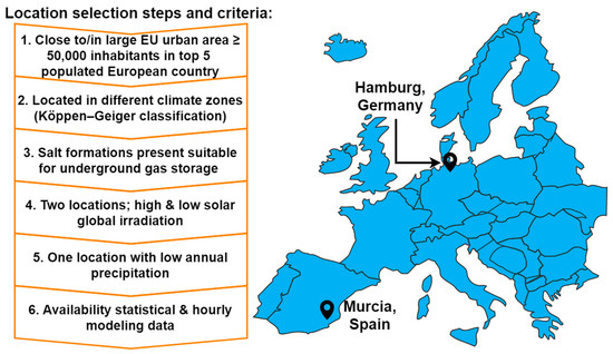
Figure 1.
Location selection steps and criteria resulted in the urban area of Hamburg in Germany and Murcia in Spain.
- Close to a large European functional urban area [12] or city with at least 50,000 inhabitants, preferably in one of Europe’s five most populous countries [103].
- Located in different European climate zones, as defined by the Köppen–Geiger climate classification [44] and supplement of [44].
- Located in a region with underground salt formations suitable for underground gas storage [104].
- One location should have a relatively high, and one location should have a relatively low solar global irradiation compared to European measurements [59,60,62].
- One location should have a relatively low annual precipitation compared to European measurements [105].
- All required statistical and hourly modeling data should be available for the selected locations (wind velocity, solar irradiation, precipitation, building energy consumption, etc.).
The urban area of Hamburg in Germany and Murcia in Spain were selected, see Figure 1. Hamburg is the cooler, windier, and rainier area; Murcia is the warmer, sunnier, and dryer area. In Appendix A.1, Table A1 shows key figures characterizing Hamburg in Germany and Murcia in Spain and their climates.
2.2.2. System Design and Dimensioning
The smart city area energy and transportation system is designed in such a way that it fulfills the following design requirements:
- uses only electricity and hydrogen as energy carriers and is all-electric in end-use
- uses only hydrogen as seasonal energy storage and fuel to power all road vehicles
- can be applied to an average European city area and is a scalable design
- can be operated in a network of multiple smart city areas and renewable hydrogen and electric energy hubs or centers [32,106,107,108,109,110]
- can be integrated into existing infrastructure and buildings
- is not dependent on an in-urban area underground hydrogen pipeline transportation network
- uses abundant renewable energy sources in Europe: local solar and large-scale wind only
- is independent of high and medium voltage electricity grids, natural gas, and district heating grids or the expansion of these.
By applying the design requirements, the integrated system design of the smart city area has the following seven major elements and functional energy performance and conversion steps (Figure 2 and Table 1):
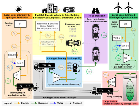
Figure 2.
Smart city area components, electricity, water, hydrogen flows, and transportation. fuel cell electric vehicles (FCEV), fuel cell electric vehicle; V2G, vehicle-to-grid.

Table 1.
Components, energy, and water flow in the smart city area (Figure 2).
- Local solar electricity and hydrogen production (orange): Local rooftop solar electricity and rainwater collection, purification, and storage systems (S1–S3) produce solar electricity (ES) and pure water (H2OS). A part of the solar electricity is directly consumed (EDC) in buildings and other sub-systems. The remaining surplus solar electricity (ES) is used with purified water (H2OS) in the hydrogen production, purification, and compression system (S4–S6) for filling tube trailers (TT1) with hydrogen (HS).
- Fuel cell electric vehicle-to-grid, building electricity consumption, and smart grid control (yellow): The smart electric grid is managed by a controller, which connects all buildings, grid-connected FCEVs (FCEV1and2), the hydrogen fueling station (HFS1-HFS4), solar electricity and hydrogen production (S1–S6), and the tube trailer filling station (SHS2) at the seasonal hydrogen storage (SHS1). The directly consumed solar electricity (EDC) is divided amongst the all-electric residential and services sector buildings (EB), HFS (EHFS), and SHS (ESHS) electricity consumption. Any shortage of electricity is met by the electricity produced from hydrogen (EV2G) through parked (at home or in public or commercial spaces) and V2G connected FCEVs (FCEV1and2).
- Hydrogen tube trailer transportation (grey): Tube trailers (TT1) towed by tube trailer tractors (TT2) transport hydrogen from either the local solar hydrogen production or the SHS to the HFS, or from the local solar hydrogen production to the SHS.
- Hydrogen fueling station (blue): Hydrogen from tube trailers is further compressed (HFS1) and stored at high pressure (HFS2). A chiller (HFS3) cools the dispensed hydrogen (HHFS), including sufficient dispensers (HFS4) to provide hydrogen for both road transportation (Hroad) and V2G (HV2G) use.
- Road transportation (purple): A fleet of road transportation FCEVs, namely passenger cars, vans, buses, trucks, and tractor-trailers.
- Large-scale and shared wind hydrogen production (green): A large-scale wind turbine park (W1) that is not located near or in smart city areas is shared with other smart city areas and renewable hydrogen hubs and consumers. All wind electricity (EW) is used with purified water (H2OW) from local surface water or seawater in hydrogen production (W4), purification (W5), and compression system (W6), which includes a water collection and purification system (W2 and W3). The hydrogen produced (HW) is stored in a large-scale underground seasonal hydrogen storage (SHS1).
- Large-scale and shared seasonal hydrogen storage (red): Large-scale underground seasonal hydrogen storage (SHS1), including a tube trailer filling and emptying station (SHS2).
The system design configuration is sufficiently flexible to allow other renewable energy sources, if present, to be used (e.g., offshore wind, biomass, or hydropower). However, this was not analyzed in this study. The smart urban area operates in a network of multiple smart urban areas, hydrogen fueling stations, other renewable hydrogen and electric energy hubs, and other hydrogen and electricity consumers (not part of this study). Hydrogen is produced within the smart urban areas from local surplus solar electricity and at large-scale wind parks. These large-scale wind parks, as well as the large-scale seasonal underground hydrogen storage, are jointly owned by the smart urban areas and other hydrogen consumers. Hydrogen is transported via tube trailers from the smart urban areas to hydrogen fueling stations, or the large-scale and shared underground seasonal hydrogen storage [104,111].
The size of a Hamburg- or Murcia-based illustrative smart city area for this study was determined using the dispersion of supermarkets and gas stations in Europe, Germany, and Spain. In the EU 28 countries, for every 2000 households, there is one medium-sized supermarket and one gas station [55,112,113,114]. In Germany and Spain, there is one gas station per 2600 and 1700 households, respectively [55,113,114]. Thus, 2000 households are a good indicator for dimensioning the smart integrated city area; see Table 2 (common parameters). This hydrogen fueling station will serve a similar vehicle population as current gasoline stations [115,116]. Total capital cost per capacity for large HFS (≥1500 kg/day) is lower than for smaller HFS [117], thus also defining the minimum size of this scalable and illustrative smart city area.
Table 2.
Characteristics of the modeled smart city areas.
On average, 2000 households in Germany and Spain correspond to, respectively, 4310 and 5083 people, with 2364 and 1846 passenger cars and 156 and 410 other vehicles, according to German and Spanish national statistical data [55,57,113,118,119,120]. See Table 2 (local parameters).
The floor area of residential and services buildings is derived from national statistical data and scaled to 2000 households: German and Spanish average household floor area S-hh is, respectively, 91.60 and 91.78 m2 [54,55]. Residential and service sector roofs will be used for solar electricity systems and rainwater collection [121,122,123,124]. Solar electricity systems are installed on all technically suitable roof areas: 9 m2 per person on residential buildings and 4 m2 per person on service sector buildings area [125,126]. Facçades are not considered.
For ease of comparison between Hamburg and Murcia, the roof area available for solar electric modules and rainwater collection in Murcia is based on the Hamburg parameters.
2.2.3. Technological and Economic Characterization of System Components in Two Scenarios
The technological and economic characteristics of the selected components will be listed according to the latest available figures in two technology development scenarios. The two scenarios, in different time frames, can be characterized as follows:
- The Near Future scenario uses current state-of-the-art renewable and hydrogen technology and current energy demand for buildings and transportation. It is an all-electric energy system, which means space heating is done using heat pumps, meeting the present heat demand for houses and buildings. Only commercially available hydrogen technologies are used. For all systems, including hydrogen technologies, current technology characteristics and cost figures are used. The Near Future scenario presents a system that could be implemented in 2020–2025.
- In the Mid Century scenario, a significant reduction in end-use energy consumption is assumed. Hydrogen and fuel cell technologies have become mature with mass production and performing on the cost and efficiency targets projected for 2050. Also, for all the other technologies, such as solar, wind, and electrolyzers, the learning curves are taken into account.
The detailed technical and cost-related parameters of the system components are presented in Appendix A.2 Table A2 and Table A3. The technology selection for the system components and sizing methods is based on the component description in [36].
2.3. Calculation Model and Hourly Simulation
Figure 3 shows the simplified simulation scheme of the calculation model, consisting of five major steps that are executed hourly for an entire year. A detailed description and input data are described in Appendix B, Table A4, Table A5 and Table A6.
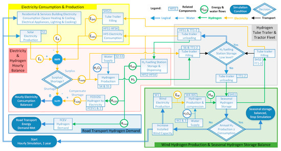
Figure 3.
Simplified hourly simulation scheme.
- Electricity consumption and production (yellow; see description in Appendix B.1)
- Road transport hydrogen demand (blue; see description in Appendix B.2)
- Electricity and hydrogen hourly balance (red; see description in Appendix B.3)
- Hydrogen tube trailer and tractor fleet (grey; see description in Appendix B.4)
- Wind hydrogen production and seasonal storage balance (green; see description in Appendix B.5)
Two sets of energy balances are calculated, on both an hourly and an annual basis (Figure 3 in red and green) for both hydrogen and electricity energy carriers. Energy consumption takes place in buildings and for mobility. Energy production is by roof-top solar and wind turbines and covers all energy consumption needs, taking into account all efficiencies of the different energy conversion and storage processes.
The amount of rooftop area available for solar electricity systems is fixed in both scenarios and locations for ease of comparison of the system performance between the two climates. The amount of installed wind capacity is the degree of freedom in the calculation model and completes the annual energy balance.
The system is simulated for five years using weather data from 2012 to 2016, which results in varying hourly electricity production consumption profiles, as well as electricity production per installed capacity. For ease of comparison between the years, the annual building electricity demand is kept constant.
2.4. Calculating the Cost of Energy
Three components of the cost of energy (CoE) will be calculated for each location in both scenarios.
- Smart city area total system cost of energy (TSCoESCA) in euros per year (Appendix C.1).
- System levelized cost of energy for electricity (SLCoEe) in euros per kWh and for hydrogen (SLCoEH) in euros per kg of hydrogen (Appendix C.2).
- Cost of energy for households (CoEhh) in euros per household per year (Appendix C.3).
2.4.1. Smart City Area Total System Cost of Energy
The TSCoESCA in euros per year is the sum of the total annual capital and operation and maintenance costs TCi (€/year) of the total number of components (n) in the smart city area. The TCi of an individual component is calculated using the annual capital cost CCi (€/year) and operation and maintenance cost OMCi (€/year); cost formulas used are listed in Appendix C.1.
The cost analyses are in constant 2015 euros. An exchange rate of 0.88 USD to 1 EUR is used as in [36]. The website [128] is used to convert all USD values to USD2015 values. A weighted average cost of capital WACC of 3% is used from Appendix A of [102].
2.4.2. System Levelized Cost of Energy
The system levelized cost of energy, for either electricity SLCoEe (€/kWh) or hydrogen SLCoEH (€/kg H2), is calculated by allocating a share of the TSCoESCA (€/year) related to either electricity TSCoESCA,e (€/year) or hydrogen consumption TSCoESCA,H (€/year). These shares are then divided by either the annual electricity consumption ECe (kWh/year) or the annual hydrogen consumption ECH (kg H2/year), resulting in, respectively, the SLCoEe (€/kWh) or the SLCoEH (€/kg H2). The cost formulas used are listed in Appendix C.2.
2.4.3. Cost of Energy for Households (Without Taxes and Levies)
Cost of Energy for a single household CoEhh (€/hh/year), here calculated without taxes and levies, consists of the cost of energy for the building energy CoEhh,B (€/hh/year) and the transportation energy CoEhh,T (€/hh/year). The cost formulas used are listed in Appendix C.3.
2.5. Inter-Annual Variability Analysis
Multiple years of hourly solar global irradiation data and hourly average wind speed data recorded at both locations will be used to analyze the inter-annual variability and its impact on the smart city area total system cost of energy (TSCoESCA).
3. Energy Balance Results and Discussion
3.1. Annual Energy Balance Results
Key energy balance parameters for FCEV2G, solar electrolyzer, and SHS usage for Hamburg and Murcia in the Near Future and Mid Century scenarios are summarized in Table 3. Detailed background figures that serve as input to Table 3 can be found in Appendix D (Figure A1, load duration curves, Figure A2, hourly electricity balance for an entire year, Figure A3, SHS storage level, and monthly hydrogen flows).
Table 3.
Key energy balance parameters for FCEVs through vehicle-to-grid (FCEV2G), solar electrolyzer, and SHS usage for Hamburg and Murcia in the Near Future and Mid Century scenarios.
The annual energy balances of Hamburg and Murcia in the Near Future and Mid Century scenarios are shown in Figure 4 and Figure 5.
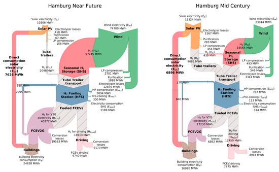
Figure 4.
Annual energy balance for Hamburg for the Near Future scenario (left) and Mid Century scenario (right).
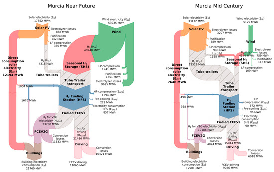
Figure 5.
Annual energy balance for Murcia for the Near Future scenario (left) and the Mid Century scenario (right).
The key energy balance parameters and annual energy balances of the years 2012–2015 show similar outcomes. Several major trends can be seen when looking at the FCEV2G, wind and solar electricity production, direct consumption of solar electricity, and seasonal hydrogen storage.
- Reliable electricity supply can be realized at all times, as extreme FCEV2G peaks never exceed 50% of the car fleet. Maximums of 760 and 772 cars, 32% and 42% of the car fleet in Hamburg and Murcia in the Near Future scenario, are reduced to 391 and 275 cars, 17% and 15% of the car fleet in the Mid Century scenario. The above maximums are extreme outliers, and values close to these occur for only a few hours per year (Figure A1).
- In the Mid Century scenario, FCEV2G usage is comparable to driving. In the Near Future scenario, the fleet average FCEV2G hours are 880 h/year compared to 440 h in Mid Century scenario at 10 kW/car output for Hamburg. For Murcia, this is 670 h and 330 h. The Mid Century scenarios’ FCEV2G hours are similar to the average driving hours for passenger cars: 310 and 280 h/year for, respectively, Hamburg and Murcia.
- The 87% higher solar electricity output in the Mid Century scenario in both locations results in less required external wind-to-hydrogen production to close the energy balance. This, together with more than a 30% reduction in building and road transportation energy consumption, and improvements in energy conversion processes, results in reductions of 70% and 90% of wind electricity production for, respectively, Hamburg and Murcia.
- The 490% higher solar hydrogen production in the Mid Century scenario in both locations compared to the Near Future scenario. Due to lower building electricity consumption and higher solar electricity production, there is more solar surplus electricity for hydrogen production. In Hamburg, solar electrolyzer power consumption always peaks in the summer’s time, whereas, in Murcia, solar electrolyzer power consumption peaks in winter (Figure A2).
- The 40% and 56% higher coverage of electricity consumption with direct solar electricity production in the Mid Century scenario in, respectively, Hamburg and Murcia compared to the Near Future scenario. Due to higher solar radiation and lower building and system electricity consumption, a higher percentage can be met directly with solar electricity. Nighttime electricity consumption has to be met with FCEV2G electricity production.
- The 15%–25% lower seasonal hydrogen storage requirements in the Mid Century scenario due to a better match of higher solar electricity production and lower building electricity demand compared to the Near Future scenario. For Hamburg, the maximum storage content of hydrogen occurs in the fall for both scenarios, whereas, in Murcia, this period shifts from spring to fall. The minimum storage content occurs in winter for both locations and scenarios. In the Mid Century scenario, a typical salt cavern [104] (Table A3) could serve approximately 23 similarly operating smart city areas in Hamburg and 40 Murcia smart city areas.
- The 40% lower seasonal hydrogen storage and FCEV2G requirements in Murcia compared to Hamburg, in all scenarios. In the Mid Century scenario, solar electricity alone is almost able to supply all of Murcia’s energy needs for buildings and road transportation (despite its 21% higher consumption of road transportation hydrogen; Appendix B.2). If approximately 15% more solar panels were to be installed, either on facades, in public spaces, or nearby solar fields, the entire energy demand could be met with solar energy. The reason for the lower SHS and FCEV2G requirements in Murcia compared to Hamburg is the better match in time (daily and seasonal) between solar electricity production and building electricity consumption. In addition, Murcia also has a relatively higher solar electricity output and lower building demand compared to Hamburg. In the Mid Century scenario in Murcia, the same solar system produces 73% more electricity than in Hamburg.
- Relatively, 70% and 30% more seasonal hydrogen storage is needed in the Mid Century scenario for, respectively, Hamburg and Murcia. Even though absolute hydrogen and electricity production, energy consumption, and seasonal hydrogen storage decrease in the Mid Century scenario, the higher dependency on solar electricity production increases the seasonal effect. Hence, there is an increase in relative seasonal hydrogen storage compared to the annual hydrogen and electricity production in the Mid Century scenario.
3.2. FCEV2G Usage and Electricity Balance Discussion and Results
Figure 6 provides further insight into seasonal and hourly FCEV2G usage. The FCEVs needed for producing V2G electricity (# cars left y-axis, % of car fleet right y-axis) are shown by means of boxplots for every hour of the day. For both locations and scenarios, usage is shown separately for both the colder winter period (in blue, left, 1 October–31 March) and the warmer summer period (in orange, right, 1 April–30 September).
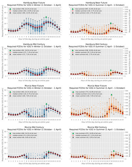
Figure 6.
Boxplots showing the hourly average FCEVs needed for producing V2G electricity (# left y-axis, % of all cars right y-axis) throughout the day during the colder winter period (in blue, left, 1 October–31 March) and the warmer “summer” period (in orange, right, 1 April–30 September) in the Near Future and Mid Century scenarios for, respectively, Hamburg and Murcia. The black crosses represent the mean values, the red lines represent the medians, and the green triangles represent the maxima. Based on a normal distribution, the bars represent the interquartile range, IQR, the difference between the first and third quartiles (Q1 and Q3), approximately 50%. The upper and lower whiskers represent the data points within the ranges [Q1–(Q1-1.5×IQR)] and [Q3+(Q3+1.5×IQR)], approximately 44%. Dots indicate outliers, outside aforementioned ranges, the remaining approx. 1%.
- Reliable electricity supply can be realized at all hours of the day, as extreme FCEV2G peaks never exceed 50% of the total car fleet. The number of cars needed to balance the system peaks in the morning (06:00–09:00) and the late afternoon/early evening (16:00–20:00) and correspond to driving rush hours. These peaks are extreme outliers, and values close to these occur for only a small number of hours per year (Figure A1).
- In Murcia, virtually no cars are required during daylight hours. This is valid in all scenarios and seasons, except for some moments. In Hamburg, this is only the case in the summer period, for both scenarios.
- Hamburg faces a greater seasonal, and Murcia a greater day-night storage challenge, particularly in the Mid Century scenario. In Hamburg, peak FCEV2G electricity production occurs in the winter period, whereas, in Murcia, the production is highest in both the summer and the winter period (see also Figure A2).
- On average, less than 22% and 13% of all cars are required during peak hours (17:00–19:00), in, respectively, the Near Future and the Mid Century scenario (black crosses).
- In Murcia, the mean FCEV2G usage is highest in summer. In Hamburg, the mean FCEV2G usage is highest in winter. Electricity demand in Murcia is dominated by space cooling, whereas, in Hamburg, it is dominated by space heating. In the Mid Century scenario, the mean daily FCEV2G usage in the winter period in Hamburg is 7.3% of all cars, whereas, in Murcia, the figure is 4.6%. In summer, this is 3% of all cars in Murcia and 2.7% of all cars in Hamburg.
- Relatively more FCEV2G electricity is produced outside regular driving hours (20:00–06:00) [129] than during regular driving hours (06:00–20:00). In the Mid Century scenario, up to 60% of all FCEV2G electricity production in Murcia takes place during the 10 night hours (20:00–06:00); the remaining 40% FCEV2G electricity is produced during the 14 regular driving hours (06:00–20:00). In Hamburg, in the Mid Century scenario, the figures are 50% during the 10 regular driving hours and 50% during the 14 regular driving hours.
4. Cost of Energy Results and Discussion
4.1. Total System Cost of Energy
The total system cost of energy per year TSCoE (k€/year) in the Near Future and Mid Century scenarios for Hamburg and Murcia is shown in Figure 7. The subsystems are grouped into hydrogen and electricity. The average component installed capacities and their total annual costs (TCi) are listed in Appendix E Table A7 and serve as input for Figure 7. The following major trends can be observed when comparing both locations and scenarios.
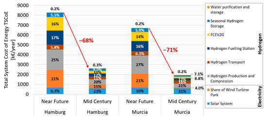
Figure 7.
Total system cost of energy (TSCoE) for the component categories in the Near Future and Mid Century scenarios for Hamburg and Murcia. The subsystems are grouped into “Hydrogen” and “Electricity”.
- The 70% reduction in TSCoE in the Mid Century compared to the Near Future scenario for both locations. Higher efficiencies, lower final energy consumption, and increased favorable match between solar electricity production and final energy consumption significantly reduce installed capacities, thus costs. Economies of scale also reduce both installed capital and operation and maintenance costs.
- The 20–30% lower TSCoE for Murcia compared to Hamburg for both scenarios. For Murcia, the TSCoE is 1.9 million euros/year in the Mid Century scenario, whereas, for Hamburg, it is 2.6 million euros/year. The reason for this is the lower final transportation and building electricity demand and lower storage and reconversion requirements.
- Variations in TSCoE from year to year are very small, 2.2–4.0% (coefficient of variation CV in Table A7 in Appendix E). This can be explained by the variations in daily and annual wind and solar electricity production, as well as the varying mismatch between solar electricity production and consumption. Seasonal hydrogen storage has relatively higher cost variations (8–12%) in comparison to other components, as the SHS is responsible for coping with all the above-mentioned variations.
- The cost of hydrogen components in the Mid Century scenario drops up to 75%. For both locations, in the Near Future scenario, the hydrogen components represent about 70% of the TSCoE; this reduces to 63% on average. As hydrogen technology is relatively new, economies of scale have a bigger impact on future cost reductions than on solar and wind electricity technology. In addition, the increase in solar output reduces storage requirements.
- Hydrogen transportation, seasonal hydrogen storage, and the solar system are the only components that share in the total costs’ relative increase compared to all other components. This is because the cost reductions for these components are relatively lower compared to the other components. The relatively higher use of seasonal hydrogen storage in the Mid Century scenario compared to the annual hydrogen production (see Section 3.1) is another contributing factor.
4.2. System Levelized Cost of Energy
The levelized and system levelized cost of electricity and hydrogen for Hamburg and Murcia in the Near Future and the Mid Century scenario are listed in Table 4. The values represent the average of the five simulated years. The levelized cost of energy (LCoE) and SLCoE parameters are calculated using the total costs (TCi, Appendix E) of the various components and the corresponding energy flows (Figure 4 and Figure 5). Detailed calculation methods can be found in Appendix C and [36].
Table 4.
Levelized (LCoE) and system levelized cost of energy (SLCoE) parameters for Hamburg and Murcia in the Near Future and Mid Century scenarios.
- The system levelized cost of energy of electricity (SLCoEe) is 239 and 176 €/MWh in the Near Future scenario for, respectively, Hamburg and Murcia, and 104 and 71 €/MWh in the Mid Century scenario. The SLCoEe is calculated by summing the costs of solar and FCEV2G electricity for buildings and dividing it by the total building electricity consumption. The total costs of solar electricity for buildings are calculated by multiplying the solar electricity consumption of buildings (Figure 4 and Figure 5) by the levelized cost of energy of solar electricity (LCoEe,S). The total FCEV2G electricity costs are calculated by multiplying the FCEV2G electricity for buildings by the system levelized cost of energy of FCEV2G electricity (SLCoEe,V2G).
- All SLCoEe reduce by approximately 60% in the Mid Century scenario compared to the Near Future scenario. Also, in Murcia, the SLCoEe is about 30% lower compared to Hamburg. In Murcia, a larger part of the building load can be directly covered by cheap and abundant solar electricity (even for hydrogen production) in both scenarios. As a result, less hydrogen production, storage, dispensing, and FCEV2G electricity are required.
- The levelized cost of energy of hydrogen from surplus solar electricity (LCoEH,S in €/kg H2) in this system is always higher than the levelized cost of energy of hydrogen from wind electricity (LCoEH,W in €/kg H2). The levelized cost of energy of hydrogen (LCoEH,W&S) before transportation and storage is based on hydrogen from both wind and solar. Even in Murcia, in the Mid Century scenario, the cost of solar electricity (LCoEe,S) is lower than the cost of wind electricity LCoEe,W. The reason for this is that a significantly higher capacity factor is achieved when the electrolyzer is connected to the wind turbine than to the solar electricity system, which only uses surplus solar electricity peaks.
- The system levelized cost of energy of hydrogen (SLCoEH) is 70–80% higher than the combined levelized cost of energy of hydrogen from solar and wind (LCoEH,W&S). The SLCoEH includes the costs of hydrogen transportation by tube trailers, seasonal and fueling station storage, and dispensing on top of the solar and wind electricity costs, and the electrolyzers and low-pressure compressors, which is only the case for the LCoEH,W&S.
4.3. LCoE and SLCoE Comparison with Other Studies
Studying “100% renewable energy systems” is relatively new [130], and no integrated transportation and energy systems are the same. Comparing the SLCOEe with other 100% renewable energy systems should be taken as a general indication since there are many differences; for example, differences in geographical locations, renewable energy sources, energy carriers, storage technologies, and simulation criteria, such as energy self-sufficiency ratios or cost input parameters. Despite such differences, we can, to a certain extent, compare some subsystem costs, onshore wind and solar electricity, stored and dispensed hydrogen, and all-time available system electricity costs, including daily and seasonal storage.
- Onshore wind electricity costs (LCoEe,W) are relatively low in comparison with other studies. Near Future scenario 24–27 €/MWh compared to 30–50 €/MWh for 2025 [131], and Mid Century scenario 16–18 €/MWh with 20–35 €/MWh for 2050 [131]. There are three reasons for this. First, the exclusion of grid connection costs of 11.5% [132,133] in this study, because of the direct coupling between the wind turbine and the electrolyzer. Second, the use of a lower WACC (3%) compared to other studies (3.5–10%) [131]. Third, the placement of wind turbines on sites with good wind conditions, resulting in good onshore wind capacity factors (33–38%).
- Rooftop solar electricity costs (LCoEe,S) are comparable to the average small rooftop and utility-scale solar electricity costs, also known as community-scale or large rooftop. Near Future scenario costs of 38–68 €/MWh are similar to 20–90 €/MWh [134,135] in 2025, and Mid Century scenario costs of 18–32 €/MWh to 15–44 €/MWh [134] in 2050. The aforementioned values from the literature have similar global horizontal irradiation, although higher WACC (4–5%) [134,135].
- Stored and dispensed hydrogen costs (SLCoEH) are similar or lower compared to other studies. Near Future scenario costs of 4.9–5.2 €/kg H2 are similar to the 4–7 €/kg H2 according to studies by the Fuel Cell Hydrogen Joint Undertaking (FCH JU) and United States Department of Energy (US DoE) [136,137,138,139]. The SLCoEH in the Mid Century scenario of 2.6–3.0 €/kg H2 is slightly lower than the US DoE targets of dispensed hydrogen (3.3–3.9 €/kg H2) [140]. The major reasons for this are the higher electricity and expensive electrolyzer costs assumed by the US DoE.
- System electricity costs (SCLoEe) are similar to or lower than those in other studies on 100% renewable energy systems, including energy and transportation. The Near Future scenario SCLoEe of 179–239 €/MWh is lower compared to the transportation and energy system of the United States National Renewable Energy Laboratory (NREL) [3]. The difference can be explained by the system’s smaller scale, higher, and older component cost figures, and the use of stationary fuel cells instead of FCEV2G technology. The Mid Century scenario SLCoE-e of 71–104 €/MWh is close to the SLCoEe of 88 €/MWh for an average European smart city area, excluding seasonal hydrogen storage [36]. Several hydrogen electricity reconversion pathways in the north of Germany have been designed and evaluated for the year 2050, including underground seasonal hydrogen storage [141]. The study reports higher values of 176–247 €/MWh, although it confirms that the costs are dominated in all pathways by the costs of purchasing electricity [141]. The authors of [102] and [142] report similar values of 75–85 €/MWh and 100 €/MWh for 100% renewable and self-sufficient energy systems in 2050. Although they have similar system electricity costs, there are several differences: [102] and [142] use different storage technologies simultaneously, include more sectors (industry, agriculture, fishing, and forestry) and renewable energy sources, and either simulate for entire countries (Germany and Spain) [102] or cities in a different continent (North America) [142].
4.4. Cost of Energy for Households (Without Taxes and Levies)
Total system costs or system levelized energy costs do not represent the combined effect of energy-saving measures, higher efficiencies, and decreased costs. Therefore, the cost of energy for an average household CoEhh (€/hh/year) is introduced as an example. To put the designed system into perspective, a comparison with today’s household energy costs would be interesting to make. This, however, is not as straightforward as it seems.
The developed system and the technologies used are very different from today’s fossil-based energy and transportation system. Cities today are not self-sufficient: They import energy from both the national and the international power and fuel network. These national and international electricity and fuel supply chain networks also come at a cost. This, however, falls outside the scope of this study.
The analyzed size of this system is very small; one could compare it to a neighborhood within these big urban areas or a very small village. In addition, only the building and the road transportation sector are analyzed and integrated here. Increasing the system size and combining several different sectors would create more integration opportunities and reduce costs. For example, the equipment could be shared to avoid underutilization.
Environmental and health savings and welfare creation (e.g., jobs) [143] compared to the present fossil system are difficult to express in costs for this specific and small-scale system. In the present situation, taxes and levies on energy can represent a great part of the energy costs for household consumers, but future estimates of taxes and levies are not within the scope of this study.
Summarizing, it is very difficult to make a fair cost comparison. Nevertheless, a very simple energy cost comparison for an average household is shown below, without any taxes or levies. The present fossil situation is compared with the designed 100% renewable system in the Near Future and the Mid Century scenarios. Additional background data for the present situation can be found in Appendix F.
The cost of energy for a single household CoEhh (€/hh/year) consists of the cost of energy for the building energy CoEhh,B (€/hh/year) and the transportation energy CoEhh,T (€/hh/year); see Table 5. The Near Future scenario CoEhh shows an increase compared to the present situation, although not by several magnitudes. For Murcia, the increase is only 30% in the Near Future scenario. This shows that even though new hydrogen technologies are used, Near Future scenario costs can come close to the present situation costs and thus give reason to explore further. We should bear in mind that the Near Future scenario only changes technologies (e.g., electric water heating and heat pumps for heating) and has no significant energy savings as in the Mid Century scenario. However, in reality, the installation of a heat pump often goes hand in hand with energy-saving measures like insulation. What’s more, any further integration with other sectors and increasing the system size could also further reduce costs.
Table 5.
The annual cost of energy for households (CoEhh) without taxes and levies for the Present, Near Future, and Mid Century scenarios in Hamburg and Murcia.
The cost of energy for households (without taxes and levies) in the Mid Century scenario is significantly lower (up to 65%) compared to the present situation—namely 770 and 520 €/year per household for Hamburg and Murcia, respectively.
Therefore, the designed system is not only renewable and reliable but also affordable.
5. Discussion
The designed and analyzed integrated transportation and energy system is an extreme hypothetical scenario, because:
- The city area is not connected to any national electricity or natural gas grid or a transportation fuel network. It is self-sufficient and stand-alone.
- Only the residential, services, and road transportation sectors have been taken into account as energy consumers (e.g., not industry, agriculture, rail, or air transportation sectors).
- Space heating and hot water production are all-electric.
- It uses a single set of technologies for road transportation, transportation fuel, energy storage, and balancing, namely hydrogen, hydrogen production, and fuel cells (FCEVs), (no batteries or Battery Electric Vehicles, BEVs).
- The city area is relatively small, based on approximately 5000 people.
In the future, a mix of multiple energy carriers, storage methods, and energy technologies could all work together. Cities in Europe already have connections to national electricity and sometimes natural gas grids. In addition, all sectors should be considered, not only the residential, services, and road transportation sectors. Increasing the system size and combining several different sectors would create more integration opportunities and could reduce costs.
However, the calculated energy costs of the designed system are affordable and in line with other studies. This gives reason to explore whether variations in system designs and balancing methods can reduce total system costs even further. The system designs and balancing methods discussed below are a non-exhaustive selection of possible options.
5.1. Other System Designs
- A national electricity grid connection would make it possible to import electricity or export peaks of solar electricity to other cities or electricity consumers in different sectors, such as industry, for example, by importing lower-cost onshore or offshore wind electricity during periods of insufficient solar electricity production (e.g., at night). This would reduce the need for hydrogen storage and FCEV2G electricity. High solar output at midday in the Mid Century scenario results in high surplus peaks to be absorbed by the solar electrolyzer. Exporting these high peaks of solar electricity to, for example, industrial cooling warehouses would reduce solar electrolyzer installed capacity and costs. Using only one electrolyzer connected to the national grid and placed next to the hydrogen station could reduce hydrogen transportation. Smart placement of electrolyzers in the electricity grid could obviate electricity grid congestion and reduce or avoid the need for expensive capacity expansion [144].
- A hydrogen pipeline network [32,145,146,147,148,149] could reduce hydrogen transportation via tube trailers and fueling station capacity. Multiple electrolyzers and hydrogen fueling stations could be interconnected via a pipeline network [150]. In this way, tube trailer hydrogen transportation could be replaced, and hydrogen transportation costs reduced. Furthermore, the partial re-compression of hydrogen when emptying a tube trailer could also be reduced or avoided altogether. The compressor could even be omitted, provided the electrolyzer hydrogen output pressure is higher than the pipeline pressure. In the case of parked FCEVs delivering V2G electricity, the fuel cell could be connected directly to the hydrogen distribution pipeline network, instead of using hydrogen from the on-board hydrogen tank [151]. Not using hydrogen from the 700 bar tank eliminates the need for refueling for V2G purposes, which in turn reduces the required capacity of hydrogen fueling stations.
- Import of low-cost renewable hydrogen could partially replace, possibly costlier, local hydrogen production and seasonal hydrogen storage, and thus total system costs. Locally and at certain times of the year, there could be insufficient solar and onshore wind sources available to produce hydrogen. Regions with abundant and low-cost hydro, solar, or wind power [152,153,154,155,156,157,158] could produce low-cost hydrogen for export. This hydrogen could be imported at demand centers instead of being produced and stored on-site. Several ideas already exist, for example, producing hydrogen (far) offshore [159] from fixed or floating wind [32,160,161,162] and solar structures [163,164], or wave energy [165] and bringing the hydrogen onshore via existing natural gas or newly built pipelines [32] or ships [166,167]. The onshore pipeline network would then distribute the hydrogen to the consumers.
- Using a lower-cost mix of renewable energy sources. In this study, the rooftop solar surface area was kept equal in both locations, even though solar electricity is more expensive in Hamburg than in Murcia. Therefore, using the lowest cost renewable energy source locally available could reduce total system costs even further. For example, hydropower, offshore wind, biomass, concentrated solar power, by-product hydrogen, or tidal or wave energy could result in lower-cost electricity than onshore wind or solar Photovoltaic (PV).
- Tailor electricity mix and its supply pattern to local demand. In Murcia, solar electricity production has a better time match with electricity consumption on both a daily and a seasonal basis. During the day, solar electricity production in summer aligns well with electricity demand in buildings for space cooling. Therefore, a lower total system cost can be achieved by tailoring the renewable energy mix to allow for a better match between the production pattern and the demand pattern [61,63,65,102,142,168,169,170,171,172,173,174,175,176,177]. This would result in lower hydrogen production, storage, transportation, fueling, and FCEV electricity production costs.
5.2. Other Balancing Methods
- Using a mix of FCEVs, BEVs, or fuel cell plug-in hybrid electric vehicle (FCPHEV) and stationary batteries [84,87,178,179,180]. Instead of only using hydrogen and FCEV2G for both daily and seasonal energy balancing, other technologies could be used in parallel. For example, batteries in BEVs or FCPHEV, as well as stationary batteries, could be used for storing or releasing peak surplus or shortage of electricity [181] for day-to-day storage. Especially in Murcia, this could result in lower total system costs, as the day-to-day storage is more prevalent in Murcia [182]. Capacity factors of electrolyzers could be improved, and so decrease costs. FCEVs and hydrogen production and storage could subsequently be used for energy balancing for longer periods, up to entire seasons [182].
- Using other CO2-free hydrogen carriers for energy transportation, short and long-term energy storage. There are several other proven and available carriers today, such as liquefied hydrogen [183,184,185,186,187], ammonia (NH3) [188], or liquid organic hydrogen carriers (LOHC) [189,190]. Transporting liquid hydrogen can be less costly compared to compressed hydrogen when volumes and distances are larger. Ammonia storage and LOHC storage are becoming commercial applications at scale, and both represent reasonable alternatives in the absence of salt caverns.
- Increase passenger car FCEV2G power output, use other FCEVs and stationary fuel cells for combined heat and power. At the moment, only passenger cars with an output of 10 kW/car while having a 100 kW fuel cell system on-board are used for FCEV2G electricity. This limitation is mainly because of potential insufficient cooling radiator capacity when parked and providing FCEV2G electricity [38]. If V2G output could be increased by enhancing cooling capacity, then proportionally fewer passenger cars would be needed. Cooling capacity could be enhanced by installing, for example, a bigger radiator and cooling fans, or by using two-phase cooling fluids with a higher cooling capacity [191]. Commercial vehicles (vans, trucks, buses) are more widely used than passenger cars, although often not during the night. By also using commercial for V2G purposes [192], the number of passenger cars would be reduced. In the case of an underground hydrogen pipeline network, stationary fuel cells [193,194,195,196,197,198] could provide heat and power to buildings, and when necessary, FCEV2Gs could provide peak power.
- Internet Technology (IT) usage for demand response forecasting, scheduling, virtual power plants, and autonomous driving. Weather and electricity demand forecasting [199,200,201,202,203,204,205,206,207,208] in combination with demand response [21,26,209,210,211] could potentially avert peaks in temporal surplus or shortage of electricity. This would reduce installed capacity cost. Combining the output of thousands of grid-connected FCEVs would create so-called virtual power plants [212,213] with potentially large capacities. Similar to mobility as a service (MaaS) [214,215,216,217,218], power or electricity as a service (PaaS or EaaS) could be introduced. To create these markets, additional pricing structures, contract types, and aggregators scheduling and operating the cars will be required [219,220,221,222]. Upcoming technologies could facilitate the scheduling of cars, for example, self-driving, free-floating, cloud-connected car-sharing fleets [223,224,225], together with inductive (wireless) self-connecting V2G infrastructure [226,227,228,229,230]. As mentioned earlier, most FCEV2G electricity is required at night, whereas most people travel and work during the day. So, even if car-sharing spreads widely and the total number of cars decreases, at night, car-sharing fleets will be used less and, therefore, will be available to provide power.
6. Conclusions
The designed and modeled system for smart urban areas is based on wind, solar, and hydrogen, where fuel cell electric vehicles provide year-round 100% renewable, reliable, and affordable energy for power, heat, and transportation in two different European climates.
The two locations in different climate zones—namely Murcia in Spain and Hamburg in Germany—were selected based on several criteria. Both are close to or in a large European urban area in one of the five most populated countries. Located in a different climate zone according to the Köppen–Geiger classification, Hamburg has a temperate oceanic climate (Cfb), and Murcia a hot semi-arid climate (BSh). Both locations have salt formations suitable for underground hydrogen gas storage. One location has a high level of solar radiation (Murcia), while the other has a low level (Hamburg).
The two designed smart city areas have the climate characteristics of Hamburg and Murcia; the dimensions are based on, respectively, German and Spanish statistical data. The smart city areas consist of 185,000 m2 floor area of residential sector buildings, and for Hamburg and Murcia, respectively, 93,000 m2 and 38,000 m2 floor area services sector buildings. Hamburg and Murcia have, respectively, a total of 2500 and 2250 fuel cell electric vehicles (FCEVs), of which 2360 and 1850 are passenger cars that can be used for producing electricity via vehicle-to-grid (V2G), so-called fuel cell electric vehicle to grid (FCEV2G). Two thousand households with a total of approximately 4300–5000 inhabitants are the minimum viable economic size for dimensioning the smart city area, as statistically, there is one gas station and one retail food shop per 2000 households. Smaller capacity fueling stations are relatively costlier.
The designed smart city area system is 100% renewable. All electricity and hydrogen can be supplied by solar and wind to fulfill the energy demand for power, heat, and transportation. The transportation and energy sectors are fully integrated, and their final energy use is all-electric. Electricity is generated by solar modules on all roofs. Surplus solar electricity is converted via water-electrolysis with rainwater into pure hydrogen. The hydrogen is compressed and transported by tube trailer modules to the nearby hydrogen fueling station (HFS) or underground seasonal hydrogen storage (SHS). At the HFS, the hydrogen is further compressed to fuel all types of FCEVs, from passenger cars, vans, buses to trucks, and tractor-trailers. In the case of a temporary shortage of solar electricity, the fuel cells in the parked and grid-connected passenger cars provide the necessary electricity (FCEV2G) by converting hydrogen from the on-board hydrogen storage tanks. At parking places at home, the office, or the local shopping area, vehicle-to-grid points connect the cars to the smart city electrical grid. The SHS is filled with hydrogen from surplus solar electricity and via a very short pipeline with hydrogen produced from wind electricity from an onshore wind turbine park. The stored hydrogen in the SHS is transported via tube trailers to the hydrogen fueling station.
The designed smart city area system is reliable at all times and independent of other energy systems and grid connections. The energy balance is simulated on an hourly basis for an entire year for a Near Future and a Mid Century scenario. Five years are simulated using climate data input from the years 2012–2016, although no significant differences in the energy balance are observed.
Reliable electricity supply can be realized at all times, as extreme peaks in the FCEV2G electricity supply never exceed 50% of the car fleet. Maximums of 32% and 42% of all cars (760 and 772 cars) in Hamburg and Murcia in the Near Future scenario drop to 17% and 15% of all cars (391 and 275 cars) in the Mid Century scenario. These maximums are extreme outliers, and values close to these only occur for a few hours per year. On average, less than 13% of all cars are required during peak hours (17:00–19:00) in the Mid Century scenario. FCEV2G usage is comparable to driving in the Mid Century scenario. There is an average of 440 FCEV2G hours per year per car compared to 310 driving hours per year for Hamburg. For Murcia, there are about 330 FCEV2G hours per year and 280 driving hours. The average number of FCEV2G hours could be reduced significantly by increasing the output per car or using other vehicles, such as buses, trucks, or vans. The passenger cars are limited to 10% (10 kW) of their maximum output (100 kW).
The underground seasonal hydrogen storage (SHS) guarantees year-round storage of hydrogen for driving and electricity production. A typical size SHS can serve around 20 smart city energy and transportation systems based on Hamburg in both scenarios, the equivalent of 86,000 people and 50,000 vehicles (passenger cars, vans, trucks, buses, and tractor-trailers). In the case of Murcia, this is about 30 smart city systems in the Near Future and 40 in the Mid Century scenarios. For the Near Future and Mid Century scenarios in Murcia, this is, respectively, the equivalent of 153,000 and 203,000 people with 68,000 and 90,000 vehicles (passenger cars, vans, trucks, buses, and tractor-trailers).
The designed smart city area system is affordable, and further cost reductions are possible. It is very difficult to make a fair cost comparison between today’s energy system and the one proposed in this study in the Mid Century scenario. Nevertheless, a very simple energy cost comparison for an average household shows that the cost of energy for households (without taxes and levies) in the Mid Century scenario can be 65% lower compared to the present situation—namely 770 and 520 €/year per household for, respectively, Hamburg and Murcia.
The developed system and the technologies used are very different from today’s fossil-based energy and transportation system. The designed and analyzed integrated transportation and energy system is an extreme hypothetical scenario because:
- The city area is not connected to any national grid; it is self-sufficient and stand-alone.
- Only the residential, services, and road transportation sectors have been taken into account as energy consumers.
- Space heating and hot water production are all-electric.
- It uses a single set of technologies for road transportation, transportation fuel, energy storage, and balancing; hydrogen, hydrogen production, and fuel cells (FCEVs and no batteries or BEVs).
- The city area is relatively small, based on approximately 5000 persons.
Increasing the system size and combining several different sectors would create more integration opportunities and could reduce costs. Environmental and health savings and welfare creation (e.g., jobs) compared to the present fossil system are difficult to express in costs for this specific and small-scale system. In the future, multiple energy carriers, storage methods, and energy technologies could work in parallel. The system levelized costs in the Mid Century scenario are 71–104 €/MWh for electricity and 2.6–3.0 €/kg for hydrogen. These results compare favorably with other studies describing fully renewable power, heat, and transportation systems. This gives reason to explore whether variations in system designs and balancing methods and technologies can further reduce total system costs.
Author Contributions
Conceptualization, V.O. and A.J.M.v.W.; methodology, V.O. and A.J.M.v.W.; software, G.S. and T.S.; validation, V.O., T.S., and A.J.M.v.W.; formal analysis, V.O., G.S., and T.S.; investigation, V.O., G.S., and T.S.; resources, V.O., G.S., and T.S.; data curation, V.O., G.S., and T.S.; writing—original draft preparation, V.O.; writing—review and editing, A.J.M.v.W.; visualization, V.O., G.S., and T.S.; supervision, A.J.M.v.W.; project administration, A.J.M.v.W.; funding acquisition, A.J.M.v.W. All authors have read and agreed to the published version of the manuscript.
Funding
This work was supported by the Dutch Research Council (NWO) [Program “Uncertainty Reduction in Smart Energy Systems (URSES)”, Project number 408-13-001].
Acknowledgments
We thank the Agencia Estatal de Meteorología (AEMET) for providing detailed weather data for multiple years and locations in Spain, which was essential for running the simulations.
Conflicts of Interest
The authors declare no conflict of interest. The funders had no role in the design of the study; in the collection, analyses, or interpretation of data; in the writing of the manuscript, or in the decision to publish the results.
Appendix A. Locations Selection, System Design, Dimensioning, and Components
Appendix A.1. Location Selection
Table A1 shows some key figures characterizing Hamburg in Germany and Murcia in Spain and their climates. Respectively, 1.8 and 1.5 million inhabitants live in urban areas [231,232,233]. Hamburg has a temperate oceanic (Cfb), and Murcia a hot semi-arid (BSh) climate, according to the Köppen–Geiger climate classification [44,234,235,236,237]. Local weather station data from 2012 to 2016 [238,239,240] are used to calculate the five-year average (µ) and annual coefficient of variation (CV, also known as the relative standard variation) of the average annual wind speed, solar global horizontal irradiation, precipitation, air temperature, daily maximum and minimum air temperatures, heating degree days (HDD) [127,241], and cooling degree days (CDD) [50,51].
Table A1.
Key figures, characterizing the climate of the two locations, Hamburg and Murcia.
Table A1.
Key figures, characterizing the climate of the two locations, Hamburg and Murcia.
| Key Figures | Locations | |
|---|---|---|
| Hamburg, Germany | Murcia, Spain | |
| No. of inhabitants of urban area (# x 1,000,000) [231,232,233] | 1.8 | 1.5 |
| Climate zone (Köppen–Geiger) (-) [44,234,235,236,237] | temperate oceanic (Cfb) | hot semi-arid (BSh) |
| Weather station data | ||
| Weather station height above sea-level (m) 1 [238,239] | 11 | 61 |
| Weather station location 1 [238,239] | 53°38′ N, 9°59′ E | 38°0′ N, 1°10′ W |
| Weather data 2012–2016 means and standard deviations | µ (CV) | µ (CV) |
| Wind speed at 10 m above ground (m/s) 1 [238,242] | 4.1 (4.3%) | 3.9 (4.3%) |
| Solar global horizontal irradiation (kWh/m2/year) [238,240] | 1020 (4%) | 1855 (1.8%) |
| Precipitation (l/m2/year) [238,240] | 735 (4.9%) | 255 (24%) |
| Air temperature (°C) [238,240] | 9.9 (5.9%) | 19.1 (2.8%) |
| Daily maximum air temperature (°C) [238,240] | 13.4 (5.1%) | 25.5 (2.2%) |
| Daily minimum air temperature (°C) [238,240] | 6.3 (8.7%) | 13.7 (4.4%) |
| Heating Degree Days (°C·day/year) 2 [238,240] | 3066 (6.5%) | 854 (16%) |
| Cooling Degree Days (°C·day/year) 2 [238,240] | 101 (24%) | 1245 (6.9%) |
1 Wind speeds measured at the nearby Almeria Airport weather station are used [242,243] because, at the Murcia weather station [239,240], wind speeds are economically less favorable for wind turbines. The non-wind weather data of the Murcia weather station is more complete than that of the Almeria Airport weather station. The Almeria Airport weather station is 21 m above sea-level and has the following coordinates: 36°50′ N, 2°21′ W. The Murcia weather station five-year average (2012–2016) and coefficient of variation of the average annual wind speed at 10 m above ground are 2.4 m/s and 2.8%, respectively. 2 Calculated with a base temperature of 18 °C as in [50,51,127].
Appendix A.2. Technological and Economic Characterization of System Components in Two Scenarios
Table A2 lists the specific energy consumption and production (SEC and SEP) (kWhe/kg H2) in the Near Future and Mid Century scenarios for the different energy conversion processes, from rainwater collection to hydrogen production, fueling, and reconversion to electricity. Alkaline water electrolysis technology is chosen as, at the moment, it is cheaper than Proton Exchange Membrane (PEM) electrolysis technology [136,244]. The electrolyzer is coupled directly to the direct current renewable energy source, so there is no AC/DC conversion needed at the electrolyzer [245]. Current state-of-the-art alkaline electrolysis technology can respond sufficiently fast [136,246,247] to short-term solar and wind power fluctuations [248,249,250,251,252,253,254]. The alkaline water electrolysis part-load efficiency curve is used from [255], and its maximum efficiency point (higher heating value (HHV)-based) is 88.8% [256,257,258] for the Near Future and 92.6% for the Mid Century scenario [258,259]. SEC for hydrogen purification is, respectively, 1.3 and 1.1 kWhe/kg H2 in the Near Future and the Mid Century scenario [260,261]. After purification, drying, and oxygen removal, the hydrogen meets the purity required for FCEVs [262] at a pressure of 15 bar and 30 bar in, respectively, the Near Future and the Mid Century scenario [136,256,257,259]. Compression SEC for all compressors (S6, W6, HFS1, and SHS2) in the Near Future scenario is in the range of 0.5–3.1 kWhe/kg H2, and in the Mid Century scenario 0.4–2.5 kWhe/kg H2 [115,263,264,265,266]. The reduction in SEC in the Mid Century scenario is due to the increase in isentropic efficiency from 60% to 80% [263] and, for compressors S6 and W6, also the higher hydrogen output pressure of the electrolyzers. The compressor at the wind park (W6) has an outlet pressure of 180 bar, the maximum SHS operating pressure [104], which is assumed to be constant in this study. The operating pressure range of hydrogen tube trailers in both scenarios is 30–500 bar with an effective storage capacity of 1014 kg H2 [136,267,268,269]. By applying a smart consolidation strategy for emptying and filling tube trailers at the SHS [263,264,270,271], the net electricity consumption is simplified as compressing hydrogen from 180 bar to 500 bar (SHS2). The electricity consumption of compressor S8 is modeled as the compression of hydrogen from the hydrogen purification output pressure of 30 bar to 500 bar. The combined compressor capacity at the HFS (HFS1) is the largest of all compressors and is modeled with a variable inlet pressure of 30–500 bar (emptying the tube trailers) and fixed outlet pressure of 875 bar of the storage (HFS2). Hydrogen cooling SEC for fueling at 700 bar is 0.20 and 0.15 kWhe/kg H2 in, respectively, the Near Future and the Mid Century scenario [177,178], and is assumed to be constant over the entire operating range of the chiller. In this study, no reduction in specific electricity consumption is foreseen in the Mid Century scenario for reverse osmosis [272,273,274]. The specific energy production SEP by the FCEV is, respectively, 20.3 and 23.6 kWhe/kg H2 in the Near Future and the Mid Century scenario. These values correspond to a tank-to-grid efficiency, ηTTG, [37] (analogous to tank-to-wheel, ηTTW, efficiency when driving) of, respectively, 51.5% and 60% (HHV) [275,276]. Furthermore, it is assumed that the SEC and SEP of the conversion processes are location independent.
Table A2.
Specific energy consumption SEC or production SEP (kWhe/kg H2) of the energy conversion processes in the smart city area for both scenarios and locations.
Table A2.
Specific energy consumption SEC or production SEP (kWhe/kg H2) of the energy conversion processes in the smart city area for both scenarios and locations.
| Label (See Figure 2 and Table 2) | Energy Conversion Processes | Specific Energy Consumption/Production (SEC/SEP) | |
|---|---|---|---|
| Near Future [kWhe/kg H2] | Mid Century [kWhe/kg H2] | ||
| W4 and S4 | Alkaline water electrolysis [246,255,256,257,258,259] | 44.4–50.0 1,2 | 42.6–47.7 1,2 |
| S5 and W5 | Hydrogen purification [260,261] | 1.3 | 1.1 |
| S6 | Compressor at local solar (500 bar) [115,263,264,265,266] | 3.0 3 | 1.8 3 |
| W6 | Compressor at wind turbine park to SHS (180 bar) [115,263,264,265,266] | 1.9 3 | 1.0 3 |
| HFS1 | Compressor at HFS ([30–500]–875 bar) [115,263,264,265,266] | 0.5–3.1 1 | 0.4–2.5 1 |
| SHS2 | Compressor at SHS (180–500 bar) [115,263,264,265,266] | 0.8 | 0.6 |
| HFS3 | Chiller [277,278] | 0.20 | 0.15 |
| S2 and W2 | Reverse Osmosis—rainwater/surface water [272,273,274] | 0.006 | 0.006 |
| FCEV1 | FCEV hydrogen to electricity [275,276,279] | 20.3 | 23.6 |
1 Direct current electrical consumption [259] at 15–100% load in the Near Future scenario and 10–100% load in the Mid Century scenario. 2 15 and 30 bar hydrogen outlet pressure in, respectively, the Near Future and the Mid Century scenario. 3 15 and 30 bar hydrogen inlet pressure in, respectively, the Near Future and the Mid Century scenario.
Table A3.
Economic parameters of the smart city area components for the Near Future and the Mid Century scenario. ICi = installed capital cost; OMi = annual operational and maintenance cost expressed as an annual percentage of the installed investment cost; LT = lifetime.
Table A3.
Economic parameters of the smart city area components for the Near Future and the Mid Century scenario. ICi = installed capital cost; OMi = annual operational and maintenance cost expressed as an annual percentage of the installed investment cost; LT = lifetime.
| Label | Subsystems and Components | Near Future | Mid Century | ||||
|---|---|---|---|---|---|---|---|
| ICi | OMi [%/year] | LTi [years] | ICi | OMi [%/year] | LTi [years] | ||
| Solar and wind electricity production | |||||||
| S1 | Solar electricity system [134,280,281] | 725 €/kWp | 2.8% | 25 | 440 €/kWp | 2.3% | 30 |
| W1 | Wind turbine park [132,133,280,281,282,283,284] | 975 €/kW | 2% | 25 | 800 €/kW | 1% | 25 |
| Hydrogen production and compression | |||||||
| S4 and S5 | Alkaline electrolyzer, including H2 purification at solar system [136,285,286,287,288] | 575 1 €/kW | 2.5% 2 | 203 | 200 €/kW | 2.5% 2 | 30 3 |
| W4 and W5 | Large-scale alkaline electrolyzer, including H2 purification at wind turbines [136,285,286,287,288] | 480 1 €/kW | 4.2% 2 | 203 | 200 €/kW | 4.4% 2 | 30 3 |
| S6 | Compressor at solar system [267,289] | 10,030/9630 €/kg H2/h 4 | 4% | 15 | 3445/3325 €/kg H2/h 4 | 2% | 15 |
| W6 | Compressor at wind turbine park to SHS [267,289] | 8250/8915 €/kg H2/h 4 | 4% | 15 | 3515/6260 €/kg H2/h 4 | 2% | 15 |
| Hydrogen transport | |||||||
| TT1 | Tube trailer storage [136,190,267] | 830 €/ kg H2 | 2% | 30 | 510 €/ kg H2 | 2% | 30 |
| TT2 | Trailer tractors [136,190,267] | 160,000 €/ tractor | 61/65% 5 | 8 6 | 160,000 €/tractor | 63/62% 5 | 8 6 |
| Hydrogen fueling station (HFS) | |||||||
| HFS1 | Compressor at HFS [267,289] | 8375/8820 €/kg H2/h 4 | 4% | 10 | 3630/3670 €/kg H2/h 4 | 2% | 10 |
| HFS2 | Storage HFS 875 bar [263,290,291] | 920 €/kg H2 | 1% | 30 | 575 €/ kg H2 | 1% | 30 |
| HFS3 | Chiller units [263,289] | 143,875 €/kg H2/min | 2% | 15 | 118,520 €/kg H2/min | 2% | 15 |
| HFS4 | Dispensers units [260,261,263,289] | 91,810 €/unit | 1.1% | 10 | 72,890 €/unit | 0.9% | 10 |
| Fuel cell electric vehicle to grid (FCEV2G) | |||||||
| FCEV1 | Replacement of fuel cell system in FCEV for V2G use [36,38,275,276,292,293,294,295,296,297,298,299,300,301,302,303,304,305,306,307] | 3970 €/100 kW | 5% | 4100 h 7 | 2650 €/100 kW | 5% | 8000 h 7 |
| FCEV2 | Smart grid, control, and V2G infrastructure [134] | 6400 €/4-point dischargers | 5% | 15 | 3200 €/4-point dischargers | 5% | 15 |
| Seasonal hydrogen storage (SHS) | |||||||
| SHS1 | SHS plant (3733 ton H2 cavern) [104] | 107,000,000 €/plant | 0.5% | 30 | 107,000,000 €/plant | 0.5% | 40 |
| SHS2 | Compressor at SHS [267,289] | 3470/3825 €/kg H2/h 4 | 4% | 15 | 1560/1665 €/kg H2/h 4 | 2% | 15 |
| Water purification and storage | |||||||
| S2 and W2 | Water purification [272] | 1,200 €/m3/day | 4.8% | 25 | 1,200 €/m3/day | 4.8% | 25 |
| S3 and W3 | Pure-water tank [121,122,123,124] | 120 €/m3 | 0.33% | 50 | 120 €/m3 | 0.33% | 50 |
1 The size of the electrolyzer at the solar system is smaller than 10 MW and, therefore, still has a higher IC in the Near Future scenario than the wind connected electrolyzer. 2 The OM includes stack replacement [36], which is calculated based on an average of 13 and 24 operating hours per day for, respectively, solar and wind-powered electrolyzers. 3 System LT is 20 and 30 years, and stack economic operating lifetime is 80,000 and 90,000 h in, respectively, the Near Future and the Mid Century scenario. 4 Figures for, respectively, Hamburg/Murcia. The compressor IC costs are dependent on, for example, mass flow capacity, discharge pressure, and pressure ratio [36]. 5 Figures for, respectively, Hamburg/Murcia. The OM is defined by the amount of hydrogen transported [36] and differs per location and scenario. 6 Lifetime of 8 years based on approximately 75,000 km/year; for the cost calculation [36], only the required driven kilometers are included, i.e., there are no “idling” costs. 7 Lifetime = economic lifetime in driving operating hours. The economic lifetime calculation when using the FCEV for both driving and V2G is explained in [36].
Appendix B. Detailed Description and Background Data of the Calculation Model and Hourly Simulation
Appendix B.1. Electricity Consumption and Production
The yellow rectangle in Figure 3 includes the electricity consumption of the services and residential buildings (EB), the HFS compressor and chiller (EHFS), the SHS compressor (ESHS), and the solar electricity production (ES). EHFS and ESHS are calculated by multiplying the hourly hydrogen throughputs by the specific energy consumption component values SEC (kWhe/kg H2) from Table A2.
The electricity consumption of the services and residential buildings (EB) in the Near Future and the Mid Century scenario is based on the energy consumption at present, called the Present Situation. Therefore, first, the Present annual specific energy consumption of the residential and services buildings SECB (kWh/m2/year) is defined for each location. The method described is applicable to any location within Europe.
Building energy consumption is divided into six energy consumption categories:
- Space heating
- Space cooling
- Water heating
- Cooking
- Lighting
- Electrical appliances
Space heating and cooling depend on the ambient temperature, which is reflected in the number of annual heating and cooling degree days (HDD and CDD; see Table A1). Hamburg and Murcia differ greatly in this regard. Also, within the respective countries (Spain and Germany), locally, the number of HDDs and CDDs [50,51,308] can differ greatly from the national weighted average [118]. Due to a lack of recent and complete studies on building energy demand relations with respect to climatic parameters, a similar method is developed as in [50,51]. For space heating for both the residential and the services sector, a relation between the specific thermal heating demand and the number of HDDs per country is established using [54,55,118]. The specific thermal heating demand is derived from the used fuel mix, useful thermal energy per fuel type, fuel demand, and floor space [54,55,118,127]. The value used as specific thermal demand for space heating in Murcia and Hamburg is taken from countries with a similar number of HDDs as Murcia and Hamburg. For Murcia, the specific thermal demand is based on the specific thermal heating demand of Cyprus, Malta, and Portugal of the available years 2010–2015. For Hamburg, it is based on the specific thermal demand of Germany, Sweden, Finland, and Lithuania.
For space cooling, the relations between CDDs, specific thermal cooling demand, and specific electricity demand from [50,51] are used.
For water heating, cooking, lighting, and electrical appliances, it is assumed the local consumption in the Murcia and Hamburg regions does not differ from the national average values [54,55].
Table A4 shows the specific annual energy consumption for buildings SECB (kWh/m2/year) per energy consumption category, and annual electricity consumption in buildings EB (MWh/year) for the residential and services sector for the Hamburg- and Murcia-based smart city areas in the Present Situation and in the Near Future and Mid Century scenarios. For the Present Situation in Hamburg and Murcia, this is 194 and 173.6 kWh/m2/year and 98.6 and 223.5 kWh/m2/year for the residential and the services sector, respectively. Combining the SECB values with the floor areas from Table A4 results in total annual energy consumption of 51,617 MWh and 26,672 MWh for Hamburg and Murcia, respectively.
SECB values in the Near Future and the Mid Century scenario are fully electric in its end-use and are defined by applying specific energy consumption savings (Table A5) to the Present SECB. Space heating SECB in the Near Future scenario for both residential and services buildings is a conversion of the Present Situation SEC with its fuel mix [54,55] and corresponding useful thermal energy fractions [127] and a heat pump Coefficient of Performance (COP) of 3.5 [309,310,311,312] into the electrical equivalent energy. For the Mid Century scenario, savings for, respectively, the residential and the services sector of 95% and 85% are achieved, based on [313]. Space cooling SECB in the Near Future remains equivalent to the Present SEC [50,51], whereas, in the Mid Century scenario, savings of 70% are realized for both sectors [309,310,313]. In the Near Future scenario, water heating and cooking SEC is realized by electrification of the Present SEC fuel mix [54,55], with the useful thermal energy fractions [127] into the electrical equivalent energy [127]. Only for water heating, savings of 50% are used in the Mid Century [313], due to the combined application of electrification, heat pump usage, solar thermal heating, and other heat recuperation techniques. By extensive use of LED technology for lighting and LED efficiency increase, savings of 20% and 80% are assumed for, respectively, the Near Future and the Mid Century scenario in both sectors [314,315,316]. A total of 0% of net savings are assumed for the SECB of electrical appliances. Although energy savings will be significant, the net savings will be zero due to an increased number and use of electrical appliances, home automation, and IT services [317,318,319].
Hamburg residential and services total SECB values in the Near Future are 83.2 and 103.3 kWh/m2/year, respectively, resulting in total energy consumption of 24,838 MWh/year. In the Mid Century scenario, SEC-B values decrease to 49.8 and 74.2 kWh/m2/year, and the energy consumption to 16,020 MWh/year. Murcia residential and services total SECB values in the Near Future are 82.9 and 170.5 kWh/m2/year, resulting in total energy consumption of 21,760 MWh/year. In the Mid Century scenario, SECB values decrease to 51.3 and 90.8 kWh/m2/year, and the energy consumption to 12,901 MWh/year.
Table A4.
Specific annual energy consumption SECB (kWh/m2/year) per energy consumption category and total annual energy consumption EB (MWh/year) in buildings for the residential and the services sector for the Hamburg- and Murcia-based smart city areas at Present and the Near Future and Mid Century scenarios.
| Energy Consumption Category | Specific Energy Consumption Buildings SECB [kWh/m2/Year] | |||||
|---|---|---|---|---|---|---|
| Hamburg, Germany | Murcia, Spain | |||||
| Present Situation | Near Future | Mid Century | Present Situation | Near Future | Mid Century | |
| Residential sector | ||||||
| Space heating [54] | 131.1 1 | 29.2 | 6.6 | 13.8 1 | 2.7 | 0.7 |
| Space cooling [51] | 0.9 b | 0.9 | 0.3 | 30.2 2 | 30.2 | 9.1 |
| Water heating [54] | 32.3 1 | 24.5 | 16.2 | 16.4 1 | 13.7 | 8.2 |
| Cooking [54] | 7.8 1 | 7.4 | 7.4 | 7.7 1 | 6.7 | 6.7 |
| Lighting [54] | 2.9 2 | 2.3 | 0.6 | 4.9 2 | 3.9 | 1.0 |
| Electrical appliances [54] | 18.9 2 | 18.9 | 18.9 | 25.7 2 | 25.7 | 25.7 |
| Total | 194.0 | 83.2 | 49.8 | 98.6 | 82.9 | 51.3 |
| Services sector | ||||||
| Space heating [55] | 80.3 1 | 18.3 | 12.1 | 48.3 1 | 11.4 | 7.2 |
| Space cooling [50] | 3.4 2 | 3.4 | 1.0 | 43.0 2 | 43.0 | 12.9 |
| Water heating [55] | 8.3 1 | 7.3 | 4.1 | 7.7 1 | 6.4 | 3.8 |
| Cooking [55] | 13.1 1 | 11.5 | 11.5 | 4.1 1 | 3.5 | 3.5 |
| Lighting 3 [55] | 28.8 2 | 23.0 | 5.8 | 71.5 2 | 57.2 | 14.3 |
| Electrical appliances [55] | 39.7 2 | 39.7 | 39.7 | 49.0 2 | 49.0 | 49.0 |
| Total | 173.6 | 103.3 | 74.2 | 223.5 | 170.5 | 90.8 |
| Total annual Energy consumption buildings EB [MWh/year] | ||||||
| Hamburg | Murcia | |||||
| Present Situation | Near Future | Mid Century | Present Situation | Near Future | Mid Century | |
| Residential | 35,541 | 15,241 | 9127 | 18,105 | 15,225 | 9422 |
| Services | 16,130 | 9597 | 6893 | 8567 | 6535 | 3479 |
| Total | 51,671 | 24,838 | 16,020 | 26,672 | 21,760 | 12,901 |
1 Fuel mix [54,55] and useful thermal energy fractions, electricity: 0.97, heat: 0.95, gas: 0.80, oil: 0.72, coal: 0.65, wood 0.55 [127]. 2 electrical energy. 3 Including the electricity used for public lighting [320].
Table A5.
Specific energy consumption savings for the Near Future and Mid Century scenarios compared to the Present Situation.
Table A5.
Specific energy consumption savings for the Near Future and Mid Century scenarios compared to the Present Situation.
| Energy Consumption Category | Specific Energy Consumption Savings Compared to Present Situation | |
|---|---|---|
| Residential Sector | Near Future | Mid Century |
| Space heating [309,310,311,312,313] | 71% 1 | 95% |
| Space cooling [51,309,310,313] | 0% | 70% |
| Water heating [54,55,127,311,313] | 24/16% 2 | 50%/50% 3 |
| Cooking [54,55,127] | 5/13% 2 | 5/13% 2 |
| Lighting [314] | 20% | 80% |
| Electrical appliances [317,318,319] | 0% 4 | 0% 4 |
| Services sector | ||
| Space heating [309,310,311,312,313] | 71% 1 | 85% |
| Space cooling [50,309,310,313] | 0% | 70% |
| Water heating [54,55,127,313] | 12/17% 2 | 50%/50% 3 |
| Cooking [54,55,127] | 12/15% 2 | 12/15% 2 |
| Lighting [314,315,316] | 20% | 80% |
| Electrical appliances [317,318,319] | 0% 4 | 0% 4 |
1 Savings due to heat pump usage, conversion of the Present Situation fuel mix [54,55] with the useful thermal energy fractions (electricity: 0.97, heat: 0.95, gas: 0.80, oil: 0.72, coal: 0.65, wood 0.55) [127] and a heat pump COP of 3.5 [309,310,311,312] into the electrical equivalent energy. 2 Hamburg/Murcia savings due to the electrification of existing primary fossil energy demand for thermal purposes. Conversion of the Present Situation fuel mix [54,55] with the useful thermal energy fractions (electricity: 0.97, heat: 0.95, gas: 0.80, oil: 0.72, coal: 0.65, wood 0.55) [127] into the electrical equivalent energy for the thermal demand [127]. 3 Hamburg/Murcia combined savings due to the application of electrification, heat pump usage, solar thermal heating, and other heat recuperation techniques. 4 Although energy savings will be significant, the net savings will be zero due to an increased number and use of electrical appliances, home automation, and IT services [317,318,319].
Hourly profiles for an entire year are constructed for each energy consumption category, type of building sector, modeled location, and scenario by multiplying the SECB values from Table A4 by normalized profiles:
- Space heating SECB is multiplied by the normalized hourly profile of aggregated natural gas consumption profiles for space heating, only in the residential [321] and the services sector [322], and the daily HDD profile with base temperature 18 °C [323]. The natural gas consumption profiles for space heating only are made by subtracting the natural gas consumption for water heating from the total natural gas consumption profiles.
- Space cooling SECB is multiplied by the hourly CDD profile with base temperature 21 °C [241,323].
- Water heating SECB is multiplied by the normalized hourly profile of the aggregated gas consumption profiles for water heating only. The natural gas consumption for water heating is extracted from the total aggregated natural gas consumption profiles during the period of 3 summer weeks (day 205 of the year onwards) with ambient temperatures above 18 °C, where it is assumed no space heating is taking place [321,322]. As the profiles are based on aggregated values, it is assumed that holiday effects are excluded.
- Cooking, lighting, and electrical appliances SECB values are multiplied by the normalized aggregated electricity consumption profiles for residential [324] and services sector buildings [325].
The solar electricity production (ES) is calculated [326,327] using the hourly global horizontal irradiation values from both Murcia and Hamburg [238,239,240]. The irradiation values are assumed to be equal in both scenarios. With the given fixed roof area available for solar electric modules (Table 2) and the solar electricity system performance ratio and efficiency of, respectively, 0.80 and 0.20 kWp/m2 in the Near Future scenario and 0.90 and 0.33 kWp/m2 in the Mid Century scenario [134,328,329,330,331,332], 11.20 and 18.67 MWp of solar power is installed in the Near Future and Mid Century for Hamburg and Murcia. The solar system inclination is 34° and 39° for, respectively, Murcia and Hamburg [333], both with an azimuth of 0°.
Appendix B.2. Road Transportation Hydrogen Demand
Annual hydrogen consumption for road transportation Hroad (kg H2/year) (blue rectangle in Figure 3) of the passenger cars, vans, trucks, tractor-trailers, and buses is calculated in Table A6 using the German and Spanish national average annual distance driven d [57,119,120] and the estimated vehicle fuel economy, specific energy consumption SECT (kg H2/100 km), in the Near Future and the Mid Century scenario [36]. For Hamburg, this results in Hroad of 479,909 kg H2/year in the Near Future scenario and decreases to 316,129 kg H2/year in the Mid Century scenario. For Murcia, this results in Hroad of 545,192 kg H2/year in the Near Future scenario and decreases to 381,732 kg H2/year in the Mid Century scenario. Hroad is then multiplied by a normalized repeating weekly fueling profile [260].
In the Near Future and the Mid Century scenario, the average annual distance driven is assumed to remain constant. The number of tube trailer tractors for hydrogen transportation and their driven kilometers are assumed to be included in the number of road tractors and the number of kilometers they are driven each year. The road vehicles are owned by either the residential or the services sector, and the road transportation energy is consumed in or between smart city areas. The final energy consumption for motorcycles is not included as it currently represents only about 1% of the total road transportation final energy consumption.
At an average annual speed of 45 km/h for passenger cars [129] in Europe and the average annual distance driven d (Table A6), there are only about 305 and 280 driving hours per year per car for, respectively, Hamburg and Murcia, mostly occurring during daylight hours [129]. For most of the non-driving time, passenger cars are mostly parked at home, the office, or close to a services sector building like a supermarket or hospital [129,334].
Table A6.
The average annual distance driven d and Near Future and Mid Century scenario-specific energy consumption of transport (SECT) for van, truck, tractor-trailer, and bus type FCEVs.
Table A6.
The average annual distance driven d and Near Future and Mid Century scenario-specific energy consumption of transport (SECT) for van, truck, tractor-trailer, and bus type FCEVs.
| Specific Energy Consumption Transportation SECT [kg H2/100 km] | Average Annual Distance Driven d [km/year/vehicle] | |||
|---|---|---|---|---|
| Vehicle Type | Near Future [36] | Mid Century [36] | Hamburg, Germany [119,120] | Murcia, Spain [57] |
| Passenger car | 1.0 | 0.6 | 13,728 | 12,535 |
| Van | 1.3 | 0.9 | 19,388 | 17,704 a |
| Truck | 4.6 | 3.7 | 31,870 b | 37,077 |
| Tractor-trailer | 6.9 | 5.5 | 96,211 | 151,513 |
| Bus | 8.6 | 6.9 | 55,883 | 147,398 |
| Hamburg, Germany | Murcia, Spain | |||
| Annual hydrogen consumption Hroad | Near Future | Mid Century | Near Future | Mid Century |
| Hydrogen [kg H2 /year] | 479,909 | 316,129 | 545,192 | 381,732 |
| Hydrogen Energy c [MWhHHV/year] | 18,913 | 12,459 | 21,486 | 15,044 |
a No data is present for vans in [57]; therefore, the same relation between the average annual distance driven of cars and vans as in Germany is used. b Including commercial vehicles 3.5–6.0 tons. c Based on a higher heating value (HHV) of 39.41 kWh/kg H2.
Appendix B.3. Electricity and Hydrogen Hourly Balance
The red rectangle, in Figure 3, includes both the electricity and the hourly balance. First, the electricity consumption of the services and residential buildings (EB), the HFS compressor and chiller (EHFS), SHS compressor (ESHS) is subtracted from the solar electricity production (ES). Any surplus solar electricity (E-surp) is converted via electrolysis and water (H2OS) into “solar” hydrogen (HS). If there is a shortage of electricity, this is compensated for by electricity from the FCEV2Gs (EV2G) by converting hydrogen (HV2G). The amount of hydrogen consumed for V2G (HV2G) is added the next day to the hydrogen fueling profile for road transportation (Hroad) and follows the same hourly pattern. HV2G and Hroad combined make up the total hydrogen dispensed at the HFS (HHFS).
Appendix B.4. Hydrogen Tube Trailer and Tractor Fleet
The grey rectangle, in Figure 3, shows the hydrogen tube trailer transportation. Once a tube trailer (TT1) is filled with “solar” hydrogen (HS), tube trailer tractors (TT2) transport the tube trailers to the HFS and unload them if the high-pressure storage tank (HFS2) is not full. If HFS2 is full, the tube trailer is emptied at the seasonal hydrogen storage (SHS1). If there is insufficient HS, and HFS2 is not full, tube trailers are filled at the SHS with the compressor (SHS2) and transported to the HFS.
Transportation of the tube trailers is modeled as one hour of unavailability; tube trailer tractor averages driving speed of 50 km/h with a single trip distance of 50 km. With a 2-h loading and unloading time [190] and 8 working hours per shift, one tractor can make two roundtrips per shift. The number of tube trailers at the three locations (solar hydrogen production, HFS, and SHS), together with the maximum number of tube trailers transported at the same time, defines the total number of tube trailers needed.
Appendix B.5. Wind Hydrogen Production and Seasonal Hydrogen Storage Balance
Wind hydrogen production and the seasonal hydrogen storage balance is shown in the green rectangle in Figure 3. As the amount of solar electricity consumption variation is limited due to the limited amount of suitable roof area, the amount of installed wind capacity, together with energy storage, closes both the hourly and the annual energy balance. The large-scale wind turbine park shared with other smart urban areas produces electricity (EW) and is directly connected to a water electrolysis and compression system (W2–W6) and has no connection with any other electricity grid. The wind energy production is sized such that the net amount of consumed hydrogen from the seasonal hydrogen storage in underground salt caverns is zero on a yearly basis. There is no curtailment of wind electricity (EW), and all electricity produced is used for the production and compression of “wind” hydrogen (HW) from water (H2OW).
The wind turbine park performance is based on the 4.2 MW land-based Enercon E-141 EP4 [335] for the Near Future scenario, and, for the Mid Century, it includes future power curve improvements based on [336]. In both scenarios, the hub height is 159 m, and the rotor diameter 141 m. The wind electricity production (EW) is calculated using the hourly wind speed values from both Almeria (see Table A1, footnote 1) and Hamburg [179,180,181,182]. The wind speeds are assumed to be equal in both scenarios and are scaled [337] to the aforementioned hub height with a roughness factor z0 of 0.13 m [338].
Appendix C. Calculating Cost of Energy
Appendix C.1. Smart City Area Total System Cost of Energy
The TSCoESCA in euros per year is the sum of the total annual capital and operation and maintenance costs TCi (€/year) of the total number of components (n) in the smart city area:
The TCi of an individual component is calculated using the annual capital cost CCi (€/year) and operation and maintenance cost OMCi (€/year):
The CCi (€/year) of a component is calculated using the annuity factor AFi (%), installed component capacity Qi (component-specific capacity), and investment cost ICi (€ per component-specific capacity):
Where the annuity factor AFi [339,340] is based on the weighted average cost of capital WACC (%) and the economic lifetime of a component LTi (years):
The annual operation and maintenance costs OMCi (€/year) are expressed as an annual percentage OMi (%) of the Qi and ICi:
Appendix C.2. System Levelized Cost of Energy
The system levelized cost of energy, for either electricity SLCoEe (€/kWh) or hydrogen SLCoEH (€/kg H2), is calculated by allocating a share of the TSCoESCA related to either electricity TSCoESCA,e or hydrogen consumption TSCoESCA,H. These shares are then divided by either the annual electricity consumption ECe (kWh/year) or the annual hydrogen consumption ECH (kg H2/year), resulting in, respectively, the SLCoEe or the SLCoEH:
Appendix C.3. Cost of Energy for Households (Without Taxes and Levies)
Cost of energy for a single household CoEhh (€/hh/year), here calculated without taxes and levies, consists of the cost of energy for the building energy CoEhh,B (€/hh/year) and the transportation energy CoEhh,T (€/hh/year).
The cost of energy for transportation energy CoEhh,T (€/hh/year) is calculated by multiplying the SLCoEH by the average annual distance driven by passenger cars dpassenger car (km/year/vehicle), the number of passenger cars per household nhh,passenger cars (#/hh), divided by the SECT,passenger cars (kg H2/100 km).
The cost of energy for building energy CoEhh,B (€/hh/year) is calculated by multiplying the SLCoEe by the residential building SECB,residential (kWh/m2/year) and the German and Spanish average household floor area Shh from Section 2.2.2.
Appendix D. Energy Balance Figures

Figure A1.
Load duration curves for the simulation, based on 2016 weather data for Hamburg (top) and Murcia (bottom) for the Near Future (left) and Mid Century scenarios (right). Direct solar use (purple), FCEV2G electricity (red), combined FCEV2G and direct solar use (blue), and the solar electrolyzer power consumption (green).

Figure A2.
Hourly electricity balances for an entire year based on 2016 weather data. From top to bottom, Hamburg in the Near Future and Mid Century and Murcia in the Near Future and Mid Century.

Figure A3.
Seasonal hydrogen storage content over the year (black line), from top to bottom Hamburg Near Future and Mid Century and Murcia Near Future and Mid Century. The annual maximum and minimum are indicated by an upward (orange) and downward (green) facing triangle. For every month, the bars on the left side (in) represent the monthly inflow of hydrogen from either solar (yellow) or wind (blue), and the bar on the right (out) shows the monthly outflow to the hydrogen fueling station.
Appendix E. Total System Cost Table
Table A7.
Installed component capacities (Q) and component total annual costs (TCi) in the smart city area Hamburg and Murcia in the Near Future and Mid Century scenario, 2012–2016 average (μ) and coefficient of variation (CV).
Table A7.
Installed component capacities (Q) and component total annual costs (TCi) in the smart city area Hamburg and Murcia in the Near Future and Mid Century scenario, 2012–2016 average (μ) and coefficient of variation (CV).
| Hamburg | Murcia | ||||||||||||||||
|---|---|---|---|---|---|---|---|---|---|---|---|---|---|---|---|---|---|
| Near Future | Mid Century | Near Future | Mid Century | ||||||||||||||
| Label | Subsystems and Components | Qi | TCi | Qi | TCi | Qi | TCi | Qi | TCi | ||||||||
| µ | CV [%] | µ [k€/yr] | CV [%] | µ | CV [%] | µ [k€/yr] | CV [%] | µ | CV [%] | µ [k€/yr] | CV [%] | µ | CV [%] | µ [k€/yr] | CV [%] | ||
| Electricity production | |||||||||||||||||
| S1 | Solar electricity system [MWp] | 11.20 | - | 690 | 18.67 | - | 600 | - | 11.20 | - | 690 | - | 18.67 | - | 600 | - | |
| W1 | Wind turbines park share [MW] | 23.36 | 8.3 | 1760 | 8.3 | 7.26 | 10.1 | 390 | 10.1 | 18.60 | 6.5 | 1400 | 6.5 | 1.43 | 16.4 | 80 | 16.4 |
| Hydrogen production and compression | |||||||||||||||||
| S4 and S5 | Alkaline electrolyzer—solar [MW] | 6.20 | 5.7 | 330 | 4.5 | 14.63 | 4 | 220 | 3.7 | 6.97 | 4.8 | 360 | 3.8 | 16.23 | 5.5 | 240 | 4.9 |
| W4 and W5 | Alkaline electrolyzer share—wind [MW] | 21.95 | 8.3 | 1150 | 8.3 | 6.95 | 10.1 | 130 | 10.1 | 17.48 | 6.5 | 920 | 6.5 | 1.36 | 16.4 | 30 | 16.4 |
| S6 | Compressor—solar [kg H2/h] | 125 | 5.7 | 150 | 3.7 | 308 | 4 | 110 | 2.6 | 140 | 4.8 | 170 | 3.1 | 342 | 5.5 | 120 | 3.6 |
| W6 | Compressor share—wind [kg H2/h] | 441 | 8.3 | 450 | 5.5 | 146 | 10.1 | 50 | 6.7 | 351 | 6.5 | 390 | 4.3 | 29 | 16.4 | 20 | 10.5 |
| Hydrogen transport | |||||||||||||||||
| TT1 | Tube trailer storage [kg H2] | 4620 | 9.5 | 270 | 9.5 | 4400 | 0 | 160 | 0 | 4400 | - | 260 | 0 | 4400 | - | 160 | - |
| TT2 | Tractor-trailers [#] | 1.9 | 6.6 | 200 | 1.7 | 1.1 | 9.5 | 120 | 2.3 | 1.4 | 8.7 | 160 | 1.9 | 1.3 | - | 140 | 0.6 |
| Hydrogen fueling station (HFS) | |||||||||||||||||
| HFS1 | Compressor [kg H2/h] | 489 | 4 | 640 | 4.6 | 240 | 3.4 | 120 | 2.4 | 343 | 9.6 | 480 | 8.3 | 172 | 5.1 | 90 | 8.4 |
| HFS2 | Stationary storage 875 bar [kg H2] | 5705 | 4.6 | 320 | 4.6 | 2715 | 3.2 | 100 | 3.2 | 4051 | 10.7 | 230 | 10.7 | 1954 | 5.5 | 70 | 5.5 |
| HFS3 | Chiller capacity [kg H2/min] | 9.5 | 4.6 | 140 | 4.6 | 4.5 | 3.2 | 60 | 3.2 | 6.7 | 10.7 | 100 | 10.7 | 3.3 | 5.5 | 40 | 5.5 |
| HFS4 | Dispensers units [#] | 29.2 | 4.6 | 340 | 4.6 | 4.5 | 3.2 | 40 | 3.2 | 20.7 | 10.7 | 240 | 10.7 | 3.3 | 5.5 | 30 | 5.5 |
| FCEV2G | |||||||||||||||||
| FCEV1 | Replacement of FC system in FCEV due to V2G use only [#100 kW systems] | 755 | 7.5 | 1190 | 1.2 | 389 | 3.3 | 230 | 0.8 | 774 | 4.3 | 750 | 1.7 | 265 | 2.2 | 140 | 1.2 |
| FCEV2 | Smart grid, Control, and V2G infrastructure [# 4-point dischargers] | 189 | 7.5 | 160 | 7.5 | 97 | 3.2 | 40 | 3.2 | 193 | 4.3 | 170 | 4.3 | 66 | 2.2 | 30 | 2.2 |
| Seasonal hydrogen storage (SHS) | |||||||||||||||||
| SHS1 | Share of SHS plant (3733 ton H2 cavern) [%] | 4.1 | 14.7 | 250 | 14.7 | 3.8 | 7.9 | 200 | 7.9 | 3.9 | 12.9 | 230 | 12.9 | 2.1 | 12.2 | 110 | 12.2 |
| SHS2 | Tube trailer filling (compressor) at SHS [kg H2/h] | 488 | 4.2 | 210 | 8.5 | 239 | 3.4 | 40 | 12.5 | 341 | 9.7 | 160 | 6.3 | 171 | 5 | 30 | 3.2 |
| Water purification and storage | |||||||||||||||||
| S2 | Reverse osmosis—solar [m3/day] | 95 | 8.3 | 12 | 8.3 | 31 | 10.1 | 4 | 10.1 | 75 | 6.4 | 10 | 6.4 | 6.2 | 16.4 | 1 | 16.4 |
| W2 | Reverse osmosis—wind [m3/day] | 6.7 | 3.8 | 0.8 | 3.8 | 20 | 4.5 | 2.6 | 4.5 | 7.6 | 5.7 | 1 | 5.7 | 21 | 2.1 | 2.6 | 2.1 |
| S3 | Pure-water tank—solar [m3] | 13 | 3.8 | 0.1 | 3.8 | 41 | 4.5 | 0.2 | 4.5 | 15 | 5.7 | 0.1 | 5.7 | 42 | 2.1 | 0.2 | 2.1 |
| W3 | Pure-water tank—wind [m3] | 189 | 8.3 | 1 | 8.3 | 63 | 10.1 | 0.3 | 10.1 | 150 | 6.4 | 0.8 | 6.4 | 12 | 16.4 | 0.1 | 16.4 |
| Total | 8290 | 4 | 2620 | 2.2 | 6710 | 3.7 | 1920 | 2.7 | |||||||||
Appendix F. Background Figures Cost of Energy for a Household
Results from previous sections serve as input for the cost of energy for a single household CoEhh (€/hh/year) in Table 5 in Section 4.4- the SECT and average annual distance driven d from Table A6, the specific energy consumption in buildings (SECB) from Table A4, the number of passenger cars and households from Table 2, the average household floor area (Shh) from Section 2.2.2, and the SLCoEe and SLCoEH from Table 4.
For the Present scenario, additional parameters are used as given in the previous sections. An average gasoline fuel consumption of a passenger car in the European Union is approximately 5.6 L/100 km [341]. Gasoline prices without taxes and levies in Germany and Spain in 2017 were 0.500 €/L and 0.544 €/L [342]. For this comparison, it is assumed that natural gas is used for space heating, water heating, cooking, and electricity for space cooling, lighting, and appliances. Average electricity prices without taxes and levies for households in Germany and Spain in 2017 were 164 €/MWh (1000–2500 kWh annual consumption) and 150 €/MWh (5000–15,000 kWh annual consumption), and natural gas prices without taxes and levies were 45 €/MWh (20–200 GJ annual consumption) and 80 €/MWh (<20 GJ annual consumption) [343,344].
References
- Rogelj, J.; Den Elzen, M.; Höhne, N.; Fransen, T.; Fekete, H.; Winkler, H.; Schaeffer, R.; Sha, F.; Riahi, K.; Meinshausen, M. Paris Agreement climate proposals need a boost to keep warming well below 2 °C. Nature 2016, 534, 631–639. [Google Scholar] [CrossRef]
- Moran, D.; Kanemoto, K.; Jiborn, M.; Wood, R.; Többen, J.; Seto, K. Carbon footprints of 13,000 cities. Environ. Res. Lett. 2018, 13, 064041. [Google Scholar] [CrossRef]
- Moran, D.; Kanemoto, K.; Jiborn, M.; Wood, R.; Többen, J.; Seto, K.C. Carbon Footprints of World Cities—Global Gridded Model of Carbon Footprints (GGMCF). 2018. Available online: http://citycarbonfootprints.info/ (accessed on 29 August 2019).
- Hughes, S.; Chu, E.K.; Mason, S.G. Introduction. In Climate Change in Cities; Hughes, S., Chu, E.K., Mason, S.G., Eds.; Springer International Publishing: Berlin/Heidelberg, Germany, 2018; pp. 1–15. [Google Scholar] [CrossRef]
- European Commission. The State of European Cities 2016: Cities Leading the Way to a Better Future; European Commission: Strasbourg, France, 2016. [Google Scholar]
- Watts, M. Commentary: Cities spearhead climate action. Nat. Clim. Chang. 2017, 7, 537–538. [Google Scholar] [CrossRef]
- International Energy Agency (IEA). Cities Lead the Way on Clean and Decentralized Energy Solutions. 2017. Available online: https://www.iea.org/newsroom/news/2017/april/cities-lead-the-way-on-clean-and-decentralized-energy-solutions.html (accessed on 29 August 2019).
- Amann, M.; Bertok, I.; Borken-Kleefeld, J.; Cofala, J.; Heyes, C.; Höglund-Isaksson, L.; Klimont, Z.; Nguyen, B.; Posch, M.; Rafaj, P.; et al. Cost-effective control of air quality and greenhouse gases in Europe: Modeling and policy applications. Environ. Model. Softw. 2011, 26, 1489–1501. [Google Scholar] [CrossRef]
- Mundaca, L.; Busch, H.; Schwer, S. ‘Successful’ low-carbon energy transitions at the community level? An energy justice perspective. Appl. Energy 2018, 218, 292–303. [Google Scholar] [CrossRef]
- C40 Cities Climate Leadership Group. C40 Cities Climate Leadership Group 2018. Available online: http://www.c40.org/about (accessed on 28 August 2019).
- United Nations. The World’s Cities in 2016; UN: New York, NY, USA, 2016. [Google Scholar]
- Eurostat. Urban Europe Statistics on Cities, Towns and Suburbs; Eurostat: Luxembourg, 2016; p. 27. [Google Scholar] [CrossRef]
- De Jong, M.; Joss, S.; Schraven, D.; Zhan, C.; Weijnen, M. Sustainable-smart-resilient-low carbon-eco-knowledge cities; Making sense of a multitude of concepts promoting sustainable urbanization. J. Clean. Prod. 2015, 109, 25–38. [Google Scholar] [CrossRef]
- International Energy Agency (IEA). Cities, Flexibility and Pathways to Carbon-Neutrality. In Nordic Energy Technology Perspectives 2016; Nordic Energy Research: Oslo, Norway, 2016. [Google Scholar] [CrossRef]
- International Energy Agency (IEA). Energy Technology Perspectives 2016—Towards Sustainable Urban Energy Systems; Nordic Energy Research: Oslo, Norway, 2016. [Google Scholar]
- Lund, P.D.; Mikkola, J.; Ypyä, J. Smart energy system design for large clean power schemes in urban areas. J. Clean. Prod. 2015, 103, 437–445. [Google Scholar] [CrossRef]
- Jacobson, M.Z.; Delucchi, M.A.; Cameron, M.A.; Frew, B.A. Low-cost solution to the grid reliability problem with 100% penetration of intermittent wind, water, and solar for all purposes. Proc. Natl. Acad. Sci. USA 2015, 112, 15060–15065. [Google Scholar] [CrossRef]
- Salvi, B.L.; Subramanian, K.A. Sustainable development of road transportation sector using hydrogen energy system. Renew. Sustain. Energy Rev. 2015, 51, 1132–1155. [Google Scholar] [CrossRef]
- Sgobbi, A.; Nijs, W.; De Miglio, R.; Chiodi, A.; Gargiulo, M.; Thiel, C. How far away is hydrogen? Its role in the medium and long-term decarbonisation of the European energy system. Int. J. Hydrogen Energy 2016, 41, 19–35. [Google Scholar] [CrossRef]
- Nastasi, B.; Lo Basso, G. Power-to-Gas integration in the Transition towards Future Urban Energy Systems. Int. J. Hydrogen Energy 2017, 42, 23933–23951. [Google Scholar] [CrossRef]
- Kylili, A.; Fokaides, P.A. European smart cities: The role of zero energy buildings. Sustain. Cities Soc. 2015, 15, 86–95. [Google Scholar] [CrossRef]
- Parra, D.; Swierczynski, M.; Stroe, D.I.; Norman, S.A.; Abdon, A.; Worlitschek, J.; O’Doherty, T.; Rodrigues, L.; Gillott, M.; Zhang, X.; et al. An interdisciplinary review of energy storage for communities: Challenges and perspectives. Renew. Sustain. Energy Rev. 2017, 79, 730–749. [Google Scholar] [CrossRef]
- Steward, D.; Zuboy, J. Community Energy: Analysis of Hydrogen Distributed Energy Systems with Photovoltaics for Load Leveling and Vehicle Refueling; National Renewable Energy Laboratory (NREL): Golden, CO, USA, 2014.
- Alavi, F.; Park Lee, E.; van de Wouw, N.; De Schutter, B.; Lukszo, Z. Fuel cell cars in a microgrid for synergies between hydrogen and electricity networks. Appl. Energy 2017, 192, 296–304. [Google Scholar] [CrossRef]
- Orecchini, F.; Santiangeli, A. Beyond smart grids—The need of intelligent energy networks for a higher global efficiency through energy vectors integration. Int. J. Hydrogen Energy 2011, 36, 8126–8133. [Google Scholar] [CrossRef]
- Calvillo, C.F.; Sánchez-Miralles, A.; Villar, J. Energy management and planning in smart cities. Renew. Sustain. Energy Rev. 2016, 55, 273–287. [Google Scholar] [CrossRef]
- Hydrogen Council. How Hydrogen Empowers the Energy Transition; Hydrogen Council: Brussels, Belgium, 2017. [Google Scholar]
- World Energy Council Netherlands. Bringing North See Energy Ashore Efficiently; World Energy Council: London, UK, 2017. [Google Scholar]
- Yoshida, T.; Kojima, K. Toyota MIRAI Fuel Cell Vehicle and Progress Toward a Future Hydrogen Society. Electrochem. Soc. Interface 2015, 24, 45–49. [Google Scholar] [CrossRef]
- Jeremy, R. The Hydrogen Economy: The Creation of the World-Wide Energy Web and the Redistribution of Power on Earth; Penguin: New York, NY, USA, 2002; pp. 63–67. [Google Scholar]
- Brandon, N.P.; Kurban, Z. Clean energy and the hydrogen economy. Philos. Trans. R. Soc. A Math Eng. Sci. 2017, 375, 20160400. [Google Scholar] [CrossRef]
- van Wijk, A.J.M. The Northern Netherlands Innovation Board. In The Green Hydrogen Economy in the Northern Netherlands—Full Report. Available online: http://profadvanwijk.com/wp-content/uploads/2017/04/NIB-BP-EN-DEF-webversie.pdf (accessed on 29 August 2019).
- Winkler-Goldstein, R.; Rastetter, A. Power to gas: The final breakthrough for the hydrogen economy? Green 2013, 3, 69–78. [Google Scholar] [CrossRef]
- Van Wijk, A.J.M.; van der Roest, E.; Boere, J. Solar Power to the People. 2018. Available online: https://www.alliedwaters.com/wp-content/uploads/2017/11/Solar-Power-to-the-People-EN.pdf (accessed on 29 August 2019).
- Staffell, I.; Scamman, D.; Velazquez Abad, A.; Balcombe, P.; Dodds, P.E.; Ekins, P.; Shah, N.; Ward, K.R. The role of hydrogen and fuel cells in the global energy system. Energy Environ. Sci. 2019, 12, 463–491. [Google Scholar] [CrossRef]
- Oldenbroek, V.; Verhoef, L.A.; van Wijk, A.J.M. Fuel cell electric vehicle as a power plant: Fully renewable integrated transport and energy system design and analysis for smart city areas. Int. J. Hydrogen Energy 2017, 42, 8166–8196. [Google Scholar] [CrossRef]
- Robledo, C.B.; Oldenbroek, V.; Abbruzzese, F.; van Wijk, A.J.M. Case study integrating a hydrogen fuel cell electric vehicle with vehicle-to-grid technology, photovoltaic power and a residential building. Appl. Energy 2018, 215, 615–629. [Google Scholar] [CrossRef]
- Oldenbroek, V.; Hamoen, V.; Alva, S.; Robledo, C.B.; Verhoef, L.A.; van Wijk, A.J.M. Fuel Cell Electric Vehicle-to-Grid: Experimental Feasibility and Operational Performance as Balancing Power Plant. Fuel Cells 2018, 18, 649–662. [Google Scholar] [CrossRef]
- International Energy Agency Hybrid & Electric Vehicle (IEA-HEV). Task 28 “Home Grids and V2X Technologies”. 2017. Available online: http://www.ieahev.org/tasks/home-grids-and-v2x-technologies-task-28/ (accessed on 28 August 2019).
- Toyota Motor Corporation. outline of the Mirai. 2014. Available online: http://newsroom.toyota.co.jp/en/download/13241306 (accessed on 28 August 2019).
- Honda Worldwide Technology Picture Book Power Exporter 9000. 2017. Available online: http://world.honda.com/powerproducts-technology/PowerExporter9000/ (accessed on 28 August 2019).
- Engineering the Extreme Capability of the Colorado ZH2. 2016. Available online: http://www.gm.com/mol/m-2016-oct-1101-zh2.html (accessed on 28 August 2019).
- Barret, S. Hyundai unveils next-gen FCEV NEXO at CES, plus home power. Fuel Cells Bull. 2018, 2018, 2. [Google Scholar] [CrossRef]
- Peel, M.C.; Finlayson, B.L.; McMahon, T.A. Updated world map of the Köppen-Geiger climate classification. Hydrol. Earth Syst. Sci. 2007, 11, 1633–1644. [Google Scholar] [CrossRef]
- Tsikaloudaki, K.; Laskos, K.; Bikas, D. On the establishment of climatic zones in Europe with regard to the energy performance of buildings. Energies 2012, 5, 32–44. [Google Scholar] [CrossRef]
- Reda, F.; Arcuri, N.; Loiacono, P.; Mazzeo, D. Energy assessment of solar technologies coupled with a ground source heat pump system for residential energy supply in Southern European climates. Energy 2015, 91, 294–305. [Google Scholar] [CrossRef]
- Eicker, U.; Colmenar-Santos, A.; Teran, L.; Cotrado, M.; Borge-Diez, D. Economic evaluation of solar thermal and photovoltaic cooling systems through simulation in different climatic conditions: An analysis in three different cities in Europe. Energy Build. 2014, 70, 207–223. [Google Scholar] [CrossRef]
- Werner, S. European space cooling demands. Energy 2016, 110, 148–156. [Google Scholar] [CrossRef]
- Dalin, P.; Nilsson, J.; Rubenhag, A. ECOHEATCOOL, Work Package 2, The European Cold Market, Final Report of WP2 of the Project Funded within the Intelligent Energy Program; Euroheat & Power: Brussels, Belgium, 2006. [Google Scholar]
- Jakubcionis, M.; Carlsson, J. Estimation of European Union service sector space cooling potential. Energy Policy 2018, 113, 223–231. [Google Scholar] [CrossRef]
- Jakubcionis, M.; Carlsson, J. Estimation of European Union residential sector space cooling potential. Energy Policy 2017, 101, 225–235. [Google Scholar] [CrossRef]
- Aebischer, B.; Catenazzi, G.; Jakob, M. Impact of Climate Change on Thermal Comfort, Heating and Cooling Energy Demand in EUROPE. Available online: https://ethz.ch/content/dam/ethz/special-interest/mtec/cepe/cepe-dam/documents/people/baebischer/Aebischer_5_110.pdf (accessed on 29 August 2019).
- Eurostat. Household Composition Statistics. 2016. Available online: http://ec.europa.eu/eurostat/statistics-explained/index.php/Household_composition_statistics (accessed on 28 August 2019).
- Enerdata. ODYSSEE Database—Households 2015. Available online: http://odyssee.enerdata.net/database/ (accessed on 28 August 2019).
- Enerdata. ODYSSEE Database—Services 2015. Available online: http://odyssee.enerdata.net/database/ (accessed on 28 August 2019).
- Eurostat. Stock of Vehicles by Category and NUTS 2 Regions 2015. Available online: http://ec.europa.eu/eurostat/web/products-datasets/-/tran_r_vehst (accessed on 28 August 2019).
- Enerdata. ODYSSEE Database—Transport 2015. Available online: http://odyssee.enerdata.net/database/ (accessed on 28 August 2019).
- Troen, I.; Petersen, E.L. European Wind Atlas; Risø National Laboratory: Roskilde, Denmark, 1989. [Google Scholar] [CrossRef]
- Šúri, M.; Huld, T.A.; Dunlop, E.D.; Ossenbrink, H.A. Potential of solar electricity generation in the European Union member states and candidate countries. Sol. Energy 2007, 81, 1295–1305. [Google Scholar] [CrossRef]
- Huld, T.; Müller, R.; Gambardella, A. A new solar radiation database for estimating PV performance in Europe and Africa. Sol. Energy 2012, 86, 1803–1815. [Google Scholar] [CrossRef]
- Huber, M.; Dimkova, D.; Hamacher, T. Integration of wind and solar power in Europe: Assessment of flexibility requirements. Energy 2014, 69, 236–246. [Google Scholar] [CrossRef]
- Huld, T.; Pinedo-Pascua, I. Photovoltaic Solar Electricity Potential in European Countries; European Commission, Joint Research Centre, Institute for Energy and Transport, Renewable Energy Unit. European Commission - Joint Research Centre: Petten, The Netherlands, 2012.
- Heide, D.; von Bremen, L.; Greiner, M.; Hoffmann, C.; Speckmann, M.; Bofinger, S. Seasonal optimal mix of wind and solar power in a future, highly renewable Europe. Renew. Energy 2010, 35, 2483–2489. [Google Scholar] [CrossRef]
- Kiviluoma, J.; Holttinen, H.; Weir, D.; Scharff, R.; Söder, L.; Menemenlis, N.; Cutululis, N.A.; Lopez, I.D.; Lannoye, E.; Estanqueiro, A.; et al. Variability in large-scale wind power generation. Wind Energy 2016, 19, 1649–1665. [Google Scholar] [CrossRef]
- Monforti, F.; Gaetani, M.; Vignati, E. How synchronous is wind energy production among European countries? Renew. Sustain. Energy Rev. 2016, 59, 1622–1638. [Google Scholar] [CrossRef]
- Pozo-Vazquez, D.; Santos-Alamillos, F.J.; Lara-Fanego, V.; Ruiz-Arias, J.A.; Tovar-Pescador, J. Hydrological, Socioeconomic and Ecological Impacts of the North Atlantic Oscillation in the Mediterranean Region. In The Impact of the NAO on the Solar and Wind Energy Resources in the Mediterranean Area; Springer: Berlin/Heidelberg, Germany, 2011; pp. 213–231. [Google Scholar]
- Santos, J.A.; Rochinha, C.; Liberato, M.L.R.; Reyers, M.; Pinto, J.G. Projected changes in wind energy potentials over Iberia. Renew. Energy 2015, 75, 68–80. [Google Scholar] [CrossRef]
- Nuño, E.; Maule, P.; Hahmann, A.; Cutululis, N.; Sørensen, P.; Karagali, I. Simulation of transcontinental wind and solar PV generation time series. Renew. Energy 2018, 118, 425–436. [Google Scholar] [CrossRef]
- Bett, P.E.; Thornton, H.E.; Clark, R.T. Using the Twentieth Century Reanalysis to assess climate variability for the European wind industry. Theor. Appl. Climatol. 2017, 127, 61–80. [Google Scholar] [CrossRef]
- Kirchner-Bossi, N.; García-Herrera, R.; Prieto, L.; Trigo, R.M. A long-term perspective of wind power output variability. Int. J. Climatol. 2015, 35, 2635–2646. [Google Scholar] [CrossRef]
- François, B. Influence of winter North-Atlantic Oscillation on Climate-Related-Energy penetration in Europe. Renew. Energy 2016, 99, 602–613. [Google Scholar] [CrossRef]
- Pfenninger, S.; Staffell, I. Long-term patterns of European PV output using 30 years of validated hourly reanalysis and satellite data. Energy 2016, 114, 1251–1265. [Google Scholar] [CrossRef]
- Brown, T.W.; Bischof-Niemz, T.; Blok, K.; Breyer, C.; Lund, H.; Mathiesen, B.V. Response to “Burden of proof: A comprehensive review of the feasibility of 100% renewable-electricity systems”. arXiv 2017, arXiv:170905716. [Google Scholar] [CrossRef]
- Zini, G.; Rosa, A.D. Hydrogen systems for large-scale photovoltaic plants: Simulation with forecast and real production data. Int. J. Hydrogen Energy 2014, 39, 107–118. [Google Scholar] [CrossRef]
- Parra, D.; Walker, G.S.; Gillott, M. Modeling of PV generation, battery and hydrogen storage to investigate the benefits of energy storage for single dwelling. Sustain. Cities Soc. 2014, 10, 1–10. [Google Scholar] [CrossRef]
- Castañeda, M.; Cano, A.; Jurado, F.; Sánchez, H.; Fernández, L.M. Sizing optimization, dynamic modeling and energy management strategies of a stand-alone PV/hydrogen/battery-based hybrid system. Int. J. Hydrogen Energy 2013, 38, 3830–3845. [Google Scholar] [CrossRef]
- Wulf, C.; Linßen, J.; Zapp, P. Review of Power-to-Gas Projects in Europe. Energy Procedia 2018, 155, 367–378. [Google Scholar] [CrossRef]
- Kilkiş, B.; Kilkiş, Ş. Hydrogen economy model for nearly net-zero cities with exergy rationale and energy-water nexus. Energies 2018, 11, 1226. [Google Scholar] [CrossRef]
- Davies, H.C.; Datardina, N. A probabilistic model for 1st stage dimensioning of renewable hydrogen transport micro-economies. Renew. Energy 2013, 60, 355–362. [Google Scholar] [CrossRef]
- Dispenza, G.; Sergi, F.; Napoli, G.; Randazzo, N.; Di Novo, S.; Micari, S.; Antonucci, V.; Andaloro, L. Development of a solar powered hydrogen fueling station in smart cities applications. Int. J. Hydrogen Energy 2017, 42, 27884–27893. [Google Scholar] [CrossRef]
- Kurtz, J.; Peters, M.; Muratori, M.; Gearhart, C. Renewable Hydrogen-Economically Viable: Integration into the U.S. Transportation Sector. IEEE Electrif. Mag. 2018, 6, 8–18. [Google Scholar] [CrossRef]
- Rahil, A.; Gammon, R.; Brown, N. Flexible operation of electrolyser at the garage forecourt to support grid balancing and exploitation of hydrogen as a clean fuel. Res. Transp. Econ. 2018, 70, 125–138. [Google Scholar] [CrossRef]
- Chrysochoidis-Antsos, N.; Liu, C.; van Wijk, A. On-site wind powered hydrogen refuelling stations—From national level to a case study in Germany. In Proceedings of the 2018 International Conference on Smart Energy Systems and Technologies (SEST), Sevilla, Spain, 10–12 September 2018; pp. 1–6. [Google Scholar] [CrossRef]
- Robinius, M.; Linßen, J.; Grube, T.; Reuß, M.; Stenzel, P.; Syranidis, K.; Kuckertz, P.; Stolten, D. Comparative Analysis of Infrastructures: Hydrogen Fueling and Electric Charging of Vehicles; Forschungszentrum Jülich GmbH Zentralbibliothek: Jülich, Germany, 2018. [Google Scholar]
- Lipman, T.E.; Edwards, J.L.; Kammen, D.M. Fuel cell system economics: Comparing the costs of generating power with stationary and motor vehicle PEM fuel cell systems. Energy Policy 2004, 32, 101–125. [Google Scholar] [CrossRef]
- Kissock, J. Combined heat and power for buildings using fuel-cell cars. In Proceedings of the ASME International Solar Energy Conference, Albuquerque, NM, USA, 14–17 June 1998; pp. 121–132. [Google Scholar]
- Williams, B.D.; Kurani, K.S. Commercializing light-duty plug-in/plug-out hydrogen-fuel-cell vehicles: “Mobile Electricity” technologies and opportunities. J. Power Sources 2007, 166, 549–566. [Google Scholar] [CrossRef]
- Kempton, W.; Tomic, J.; Letendre, S.; Brooks, A.; Lipman, T. Vehicle-to-Grid Power: Battery, Hybrid, and Fuel Cell Vehicles as Resources for Distributed Electric Power in California; Institute of Transportation Studies: Davis, CA, USA, 2001. [Google Scholar]
- Kempton, W.; Tomić, J. Vehicle-to-grid power fundamentals: Calculating capacity and net revenue. J. Power Sources 2005, 144, 268–279. [Google Scholar] [CrossRef]
- Garmsiri, S.; Koohi-Fayegh, S.; Rosen, M.A.; Smith, G.R. Integration of transportation energy processes with a net zero energy community using captured waste hydrogen from electrochemical plants. Int. J. Hydrogen Energy 2016, 41, 8337–8346. [Google Scholar] [CrossRef]
- Alanne, K.; Cao, S. Zero-energy hydrogen economy (ZEH2E) for buildings and communities including personal mobility. Renew. Sustain. Energy Rev. 2017, 71, 697–711. [Google Scholar] [CrossRef]
- Cao, S. Comparison of the energy and environmental impact by integrating a H2 vehicle and an electric vehicle into a zero-energy building. Energy Convers. Manag. 2016, 123, 153–173. [Google Scholar] [CrossRef]
- Fernandes, A.; Woudstra, T.; van Wijk, A.; Verhoef, L.; Aravind, P.V. Fuel cell electric vehicle as a power plant and SOFC as a natural gas reformer: An exergy analysis of different system designs. Appl. Energy 2016, 173, 13–28. [Google Scholar] [CrossRef]
- Toyota Motor Corporation. Seven-Eleven Japan and Toyota to Launch Joint Next-Generation Convenience Store Project in Autumn 2019 toward Greater CO2 Emissions Reduction. Toyota Newsroom 2018. Available online: https://newsroom.toyota.co.jp/en/corporate/22833613.html (accessed on 28 August 2019).
- Cao, S.; Alanne, K. Technical feasibility of a hybrid on-site H2 and renewable energy system for a zero-energy building with a H2 vehicle. Appl. Energy 2015, 158, 568–583. [Google Scholar] [CrossRef]
- Oldenbroek, V.; Wijtzes, S.; Wijk A van Blok, K. Fuel cell electric vehicle to grid & H2: Balancing national electricity, heating & transport systems a scenario analysis for Germany in the year 2050. In Proceedings of the 2017 IEEE Green Energy and Smart Systems Conference, Long Beach, CA, USA, 6–7 November 2017; pp. 1–6. [Google Scholar] [CrossRef]
- Lord, A.S.; Kobos, P.H.; Borns, D.J. Geologic storage of hydrogen: Scaling up to meet city transportation demands. Int. J. Hydrogen Energy 2014, 39, 15570–15582. [Google Scholar] [CrossRef]
- Mukherjee, U.; Maroufmashat, A.; Ranisau, J.; Barbouti, M.; Trainor, A.; Juthani, N.; El-Shayeb, H.; Michael Fowler, M. Techno-economic, environmental, and safety assessment of hydrogen powered community microgrids; case study in Canada. Int. J. Hydrogen Energy 2017, 42, 14333–14349. [Google Scholar] [CrossRef]
- Farahani, S.S.; Veen R van der Oldenbroek, V.; Alavi, F.; Lee, E.H.P.; van de Wouw, N.; van Wijk, A.; De Schutter, B.; Lukszo, Z. A Hydrogen-Based Integrated Energy and Transport System: The Design and Analysis of the Car as Power Plant Concept. IEEE Syst. Man Cybern. Mag. 2019, 5, 37–50. [Google Scholar] [CrossRef]
- Marchenko, O.V.; Solomin, S.V. Modeling of hydrogen and electrical energy storages in wind/PV energy system on the Lake Baikal coast. Int. J. Hydrogen Energy 2017, 42, 9361–9370. [Google Scholar] [CrossRef]
- Shimizu, T.; Tsukushi, Y.; Hasegawa, K.; Ihara, M.; Okubo, T.; Kikuchi, Y. A region-specific analysis of technology implementation of hydrogen energy in Japan. Int. J. Hydrogen Energy 2019, 44, 19434–19451. [Google Scholar] [CrossRef]
- Jacobson, M.Z.; Delucchi, M.A.; Cameron, M.A.; Mathiesen, B.V. Matching demand with supply at low cost in 139 countries among 20 world regions with 100% intermittent wind, water, and sunlight (WWS) for all purposes. Renew. Energy 2018, 123, 236–248. [Google Scholar] [CrossRef]
- Eurostat. Population Change—Demographic Balance and Crude Rates at National Level. 2017. Available online: http://appsso.eurostat.ec.europa.eu/nui/show.do?dataset=demo_gind (accessed on 28 August 2019).
- Bünger, U.; Michalski, J.; Crotogino, F.; Kruck, O. Compendium of Hydrogen Energy. In Large-Scale Underground Storage of Hydrogen for the Grid Integration of Renewable Energy and Other Applications; Woodhead Publishing: Sawston, UK, 2016; pp. 133–163. [Google Scholar] [CrossRef]
- European Environment Agency. Average annual precipitation 1940–1995 Europe. 2011. Available online: https://www.eea.europa.eu/themes/water/water-resources/figures-and-maps/precipitation/view (accessed on 28 August 2019).
- Andrews, J.; Shabani, B. Re-envisioning the role of hydrogen in a sustainable energy economy. Int. J. Hydrogen Energy 2012, 37, 1184–1203. [Google Scholar] [CrossRef]
- Maroufmashat, A.; Fowler, M.; Sattari Khavas, S.; Elkamel, A.; Roshandel, R.; Hajimiragha, A. Mixed integer linear programing based approach for optimal planning and operation of a smart urban energy network to support the hydrogen economy. Int. J. Hydrog. Energy 2016, 41, 7700–7716. [Google Scholar] [CrossRef]
- E3MLab. PRIMES MODEL VERSION 6, 2016-2017 Detailed Model Description—Hydrogen Supply Sub-Model; E3MLab: Athens, Greece, 2017; pp. 197–200. [Google Scholar]
- Maroufmashat, A.; Elkamel, A.; Fowler, M.; Sattari, S.; Roshandel, R.; Hajimiragha, A.; Walker, S.; Entchev, E. Modeling and optimization of a network of energy hubs to improve economic and emission considerations. Energy 2015, 93, 2546–2558. [Google Scholar] [CrossRef]
- Hydrogen Hub. Local Hydrogen Hubs 2018. Available online: http://www.hydrogenhub.org/#locally (accessed on 28 August 2019).
- Kostowski, W.; Lepszy, S.; Uthke, W.; Chromik, M.; Wierciński, A.; Foltynowicz, M.; Stendera, T. Effectiveness of the Hydrogen Production, Storage and Utilization Chain BT—Renewable Energy Sources: Engineering, Technology, Innovation; Mudryk, K., Werle, S., Eds.; Springer International Publishing: Berlin/Heidelberg, Germany, 2018; pp. 321–331. [Google Scholar]
- EY; Cambridge Econometrics Ltd.; Arcadia International, European Commission. The Economic Impact of Modern Retail on Choice and Innovation in the EU Food Sector—Final Report; Publications Office of the European Union: Luxembourg, Luxembourg, 2011. [Google Scholar]
- Eurostat. Number of Private Households by Household Composition, Number of Children and Age of Youngest Child (1 000). 2015. Available online: http://ec.europa.eu/eurostat/en/web/products-datasets/-/LFST_HHNHTYCH (accessed on 28 August 2019).
- FuelsEurope—Division of the European Petroleum Refiners Association. Number of Petrol Stations in Europe End of 2015; FuelsEurope: Brussels, Belgium, 2016. [Google Scholar]
- Chen, T.-P. Final Report Hydrogen Delivery Infrastructure Options Analysis; DOE award number: DE-FG36–05GO15032; Department of Energy (DOE): San Francisco, CA, USA, 2008.
- Muratori, M.; Bush, B.; Hunter, C.; Melaina, M.W. Modeling hydrogen refueling infrastructure to support passenger vehicles. Energies 2018, 11, 1171. [Google Scholar] [CrossRef]
- Melaina, M.; Penev, M. Hydrogen Station Cost Estimates: Comparing Hydrogen Station Cost Calculator Results with Other Recent Estimates; National Renewable Energy Laboratory (NREL): Golden, CO, USA, 2013.
- Enerdata. ODYSSEE Database—Macro 2015. Available online: http://odyssee.enerdata.net/database/ (accessed on 28 August 2019).
- Kraftfahrt-Bundesamt. Verkehr in Kilometern der deutschen Kraftfahrzeuge im Jahr 2015. 2016. Available online: https://www.kba.de/DE/Statistik/Kraftverkehr/VerkehrKilometer/2015/2015_vk_kurzbericht_pdf.pdf?__blob=publicationFile&v=1 (accessed on 28 August 2019).
- Kraftfahrt-Bundesamt. Der Fahrzeugbestand im Überblick am 1. Januar 2016 gegenüber 1. Januar 2015. 2016. Available online: https://www.kba.de/SharedDocs/Pressemitteilungen/DE/2016/pm_08_16_bestand_01_16_pdf.pdf?__blob=publicationFile&v=8 (accessed on 28 August 2019).
- Sharma, A.K.; Begbie, D.; Gardner, T. Rainwater Tank Systems for Urban Water Supply: Design, Yield, Energy, Health Risks, Economics and Social Perceptions; IWA Publishing: London, UK, 2015. [Google Scholar]
- Sharma, A.K.; Cook, S.; Gardner, T.; Tjandraatmadja, G. Rainwater tanks in modern cities: A review of current practices and research. J. Water Clim. Chang. 2016, 7, 445–466. [Google Scholar] [CrossRef]
- Siems, R.; Sahin, O. Energy intensity of residential rainwater tank systems: Exploring the economic and environmental impacts. J. Clean. Prod. 2016, 113, 251–262. [Google Scholar] [CrossRef]
- Gurung, T.R.; Umapathi, S.; Sharma, A.K. Economics of Scale Analysis of Communal Rainwater Tanks; Urban Water Security Research Alliance: Brisbane, Australia, 2012. [Google Scholar]
- Gutschner, M.; Nowak, S.; Ruoss, D.; Toggweiler, P.; Schoen, T. Potential for building integrated photovoltaics, IEA-PVPS Task 7; IEA Photovoltaic Power Systems Programme (PVPS), NET Nowa Energy & Technology Ltd: St. Ursen, Switzerland, 2002. [Google Scholar]
- International Energy Agency (IEA). Energy Technology Perspectives 2016: Towards Sustainable Urban Energy Systems, Annex H Rooftop Solar PV Potential in Cities; IEA Publications: Paris, France, 2016. [Google Scholar]
- Enerdata. Definition of data and energy efficiency indicators in ODYSSEE data base. Available online: http://www.odyssee-mure.eu/private/definition-indicators.pdf (accessed on 29 August 2019).
- Bureau of Labor Statistics (BLS)—U.S. Department of Labor. Inflation Calculator. 2017. Available online: https://www.bls.gov/data/inflation_calculator.htm (accessed on 28 August 2019).
- Pasaoglu, G.; Fiorello, D.; Martino, A.; Zani, L.; Zubaryeva, A.; Thiel, C. Driving and Parking Patterns of European Car Drivers—A Mobility Survey; Joint Research Centre of the European Commission: Brussels, Belgium, 2012; 66. [Google Scholar] [CrossRef]
- Khalilpour, K.R. Chapter 16—The Transition From X% to 100% Renewable Future: Perspective and Prospective. In Polygeneration with Polystorage for Chemical and Energy Hubs; Academic Press: Cambridge, MA, USA, 2019; pp. 513–549. [Google Scholar] [CrossRef]
- Agora Energiewende. Future Cost of Onshore Wind. Recent Auction Results, Long-Term Outlook and Implications for Upcoming German Auctions; Agora Energiewende: Berlin, Germany, 2017. [Google Scholar]
- International Renewable Energy Agency (IRENA). Renewable Energy Cost Analysis—Wind Power; International Renewable Energy Agency: Abu Dhabi, United Arab Emirates, 2012. [Google Scholar]
- International Renewable Energy Agency (IRENA). Renewable Power Generation Costs in 2014; International Renewable Energy Agency: Abu Dhabi, United Arab Emirates, 2015. [Google Scholar]
- Agora Energiewende. Current and Future Cost of Photovoltaics; Long-Term Scenarios for Market Development, System Prices and LCOE of Utility Scale PV-Systems; Agora Energiewende: Berlin, Germany, 2015. [Google Scholar]
- Kost, C.; Shammugamverena, S.; Jülch, V.; Nhuyen, H.-T.; Schlegl, T. Levelized Cost of Electricity Renewable Energy Technologies; Fraunhofer Institute for Solar Energy Systems ISE: Karlsruhe, Germany, 2018. [Google Scholar]
- Chardonnet, C.; Vos LDe Genoese, F.; Roig, G.; Bart, F.; Ha, T.; Van Genabet, B. Early Business Cases for H2 in Energy Storage and more Broadly Power to H2 Applications; Tractebel, Hinicio, Fuel Cell Hydrogen Joint Undertaking (FCH-JU): Brussels, Belgium, 2017. [Google Scholar]
- National Renewable Energy Laboratory (NREL). H2A analysis, Production Case Studies: Current Distributed Hydrogen Production from Grid PEM Electrolysis Version 3.2018. 2018. Available online: https://www.alliedwaters.com/wp-content/uploads/2017/11/Solar-Power-to-the-People-EN.pdf (accessed on 29 August 2019).
- National Renewable Energy Laboratory (NREL). H2A Analysis, Production Case Studies: Current Central Hydrogen Production from Polymer Electrolyte Membrane (PEM) Electrolysis Version 3.2018. 2018. Available online: https://www.nrel.gov/hydrogen/assets/docs/current-central-pem-electrolysis-v3-2018.xlsm (accessed on 29 August 2019).
- Strategic Analysis (SA), National Renewable Energy Laboratory (NREL). PEM Electrolysis H2A Production Case Study Documentation; National Renewable Energy Laboratory (NREL): Golden, CO, USA, 2013.
- Fuel Cell Technologies Office (FCTO)—U.S. Department of Energy (DOE). Multi-Year Research, Development, and Demonstration (MYRD&D) Plan—Section 3.1 Hydrogen Production. 2015. Available online: https://www.alliedwaters.com/wp-content/uploads/2017/11/Solar-Power-to-the-People-EN.pdf (accessed on 29 August 2019).
- Welder, L.; Stenzel, P.; Ebersbach, N.; Markewitz, P.; Robinius, M.; Emonts, B.; Stolten, D. Design and evaluation of hydrogen electricity reconversion pathways in national energy systems using spatially and temporally resolved energy system optimization. Int. J. Hydrogen Energy 2018, 44, 9594–9607. [Google Scholar] [CrossRef]
- Jacobson, M.Z.; Cameron, M.A.; Hennessy, E.M.; Petkov, I.; Meyer, C.B.; Gambhir, T.K.; Maki, A.T.; Pfleeger, K.; Clonts, H.; McEvoy, A.L.; et al. 100% clean and renewable Wind, Water, and Sunlight (WWS) all-sector energy roadmaps for 53 towns and cities in North America. Sustain. Cities Soc. 2018. [Google Scholar] [CrossRef]
- Steinberger-Wilckens, R.; Sampson, B. Chapter 8—Market, Commercialization, and Deployment—Toward Appreciating Total Owner Cost of Hydrogen Energy Technologies; Academic Press: Cambridge, MA, USA, 2019; pp. 383–403. [Google Scholar] [CrossRef]
- Robinius, M.; Raje, T.; Nykamp, S.; Rott, T.; Müller, M.; Grube, T.; Katzenbach, B.; Küppers, S.; Stolten, D. Power-to-Gas: Electrolyzers as an alternative to network expansion—An example from a distribution system operator. Appl. Energy 2018, 210, 182–197. [Google Scholar] [CrossRef]
- Hermkens, R.; Jansma, S.; van der Laan, M.; de Laat, H.; Pilzer, B.; Pulles, K. Toekomstbestendige gasdistributienetten—Netbeheer Nederland; Kiwa Technology B.V.: Apeldoorn, The Netherlands, 2018. [Google Scholar]
- Sadler, D.; Cargill, A.; Crowther, M.; Rennie, A.; Watt, J.; Burton, S.; Haines, M. H21 Leeds City Gate; Northern Gas Networks: Leeds, UK, 2016. [Google Scholar]
- Northern Gas Networks. H21 North of England—Deep Decarbonisation of Heat to Meet Climate Change Targets. 2018. Available online: https://www.northerngasnetworks.co.uk/event/h21-launches-national/ (accessed on 29 August 2019).
- Baufumé, S.; Grüger, F.; Grube, T.; Krieg, D.; Linssen, J.; Weber, M.; Hake, J.-F.; Stolten, D. GIS-based scenario calculations for a nationwide German hydrogen pipeline infrastructure. Int. J. Hydrogen Energy 2013, 38, 3813–3829. [Google Scholar] [CrossRef]
- Johnson, N.; Ogden, J. A spatially-explicit optimization model for long-term hydrogen pipeline planning. Int. J. Hydrogen Energy 2012, 37, 5421–5433. [Google Scholar] [CrossRef]
- Brey, J.J.; Carazo, A.F.; Brey, R. Exploring the marketability of fuel cell electric vehicles in terms of infrastructure and hydrogen costs in Spain. Renew. Sustain. Energy Rev. 2018, 82, 2893–2899. [Google Scholar] [CrossRef]
- Robledo, C.B.; Oldenbroek, V.; Seiffers, J.; Seiffers, M.; van Wijk, A.J.M. Performance of a Lightweight Fuel Cell/Battery Hybrid Electric Vehicle Operating in Vehicle-to-Grid. Fuel Cell Semin. Energy Expo. 2017. Available online: https://pure.tudelft.nl/portal/en/activities/performance-of-a-lightweight-fuel-cellbattery-hybrid-electric-vehicle-operating-in-vehicletogrid(173c09eb-58f8-459a-8631-b11d9bd808ae).html (accessed on 29 August 2019).
- Kamiya, S.; Nishimura, M.; Harada, E. Study on introduction of CO2 free energy to Japan with liquid hydrogen. Phys. Procedia 2015, 67, 11–19. [Google Scholar] [CrossRef]
- Kan, S.; Shibata, Y. Evaluation of the Economics of Renewable Hydrogen Supply in the APEC Region; The Institute of Energy Economics, Japan (IEEJ): Tokyo, Japan, 2018. [Google Scholar]
- Mizuno, Y.; Ishimoto, Y.; Sakai, S.; Sakata, K. Economic analysis on internatiol hydrogen energy carrier supply chains. J. Jpn. Soc. Energy Resour. 2016, 38, 11–17. [Google Scholar]
- Chapman, A.J.; Fraser, T.; Itaoka, K. Hydrogen import pathway comparison framework incorporating cost and social preference: Case studies from Australia to Japan. Int. J. Energy Res. 2017. [Google Scholar] [CrossRef]
- Takaoka, Y.; Kagaya, H.; Saeed, A.; Nishimura, M. Introduction to a Liquefied Hydrogen Carrier for a Pilot Hydrogen Energy Supply Chain (HESC); Kawasaki Heavy Industries, Ltd: Tokyo, Japan, 2017. [Google Scholar]
- Timmerberg, S.; Kaltschmitt, M. Hydrogen from renewables: Supply from North Africa to Central Europe as blend in existing pipelines—Potentials and costs. Appl. Energy 2019, 237, 795–809. [Google Scholar] [CrossRef]
- Schmidt, J.; Gruber, K.; Klingler, M.; Klöckl, C.; Camargo, L.R.; Regner, P.; Turkovska, O.; Wehrle, S.; Wetterlund, E. A new perspective on global renewable energy systems: Why trade in energy carriers matters. Energy Environ. Sci. 2019. [Google Scholar] [CrossRef]
- Blanco-Fernández, P.; Pérez-Arribas, F. Offshore facilities to produce hydrogen. Energies 2017, 10, 783. [Google Scholar] [CrossRef]
- Meier, K. Hydrogen production with sea water electrolysis using Norwegian offshore wind energy potentials: Techno-economic assessment for an offshore-based hydrogen production approach with state-of-the-art technology. Int. J. Energy Environ. Eng. 2014, 5, 1–12. [Google Scholar] [CrossRef]
- Det Norske Veritas Germanischer Lloyd (DNV GL). Offshore Production of Renewable Hydrogen, Summer Project 2015; DNV GL AS: Høvik, Norway, 2015. [Google Scholar]
- Jørg, A.; Eijgelaar, M.; Hektor, E.A. Hydrogen as an energy carrier - An evaluation of emerging hydrogen value chains; DNV GL AS: Høvik, Norway, 2018. [Google Scholar]
- Oceans of Energy. Offshore Floating Solar 2018. Available online: https://oceansofenergy.blue/ (accessed on 28 August 2019).
- Pouran, H.M. From collapsed coal mines to floating solar farms, why China’s new power stations matter. Energy Policy 2018. [Google Scholar] [CrossRef]
- Serna, Á.; Tadeo, F. Offshore hydrogen production from wave energy. Int. J. Hydrogen Energy 2014. [Google Scholar] [CrossRef]
- Maekawa, K.; Takeda, M.; Hamaura, T.; Suzuki, K.; Miyake, Y.; Matsuno, Y.; Fujikawa, S.; Kumakura, H. First experiment on liquid hydrogen transportation by ship inside Osaka bay. In IOP Conf. Ser. Mater. Sci. Eng.; 2017. [Google Scholar] [CrossRef]
- Wilhelmsen, Equinor, Moss Maritime, Det Norske Veritas Germanischer Lloyd (DNV GL). New Design Makes Liquefied Hydrogen Bunker Vessels a Reality. 2019. Available online: https://www.wilhelmsen.com/media-news-and-events/press-releases/2019/new-design-makes-liquefied-hydrogen-bunker-vessels-a-reality/ (accessed on 28 August 2019).
- Rasmussen, M.G.; Andresen, G.B.; Greiner, M. Storage and balancing synergies in a fully or highly renewable pan-European power system. Energy Policy 2012. [Google Scholar] [CrossRef]
- Gils, H.C.; Scholz, Y.; Pregger, T.; Luca de Tena, D.; Heide, D. Integrated modelling of variable renewable energy-based power supply in Europe. Energy 2017, 123, 173–188. [Google Scholar] [CrossRef]
- Pietzcker, R.C.; Ueckerdt, F.; Carrara, S.; de Boer, H.S.; Després, J.; Fujimori, S.; Johnson, N.; Kitous, A.; Scholz, Y.; Sullivan, P. System integration of wind and solar power in integrated assessment models: A cross-model evaluation of new approaches. Energy Econ. 2017, 64, 583–599. [Google Scholar] [CrossRef]
- Jacobson, M.Z.; Delucchi, M.A.; Cameron, M.A.; Mathiesen, B.V.; Appendix, A. Supplementary data - Matching demand with supply at low cost in 139 countries among 20 world regions with 100% intermittent wind, water, and sunlight (WWS) for all purposes. Renew. Energy 2018, 123, 236–248. [Google Scholar] [CrossRef]
- Slusarewicz, J.H.; Cohan, D.S. Assessing solar and wind complementarity in Texas. Renew. Wind Water Sol. 2018, 5, 7. [Google Scholar] [CrossRef]
- Budischak, C.; Sewell, D.; Thomson, H.; Mac, H.L.; Veron, D.E.; Kempton, W. Cost-minimized combinations of wind power, solar power and electrochemical storage, powering the grid up to 99.9% of the time. J. Power Sources 2013, 225, 60–74. [Google Scholar] [CrossRef]
- Deetjen, T.A.; Martin, H.; Rhodes, J.D.; Webber, M.E. Modeling the optimal mix and location of wind and solar with transmission and carbon pricing considerations. Renew. Energy 2018, 120, 35–50. [Google Scholar] [CrossRef]
- Schaber, K.; Steinke, F.; Mühlich, P.; Hamacher, T. Parametric study of variable renewable energy integration in Europe: Advantages and costs of transmission grid extensions. Energy Policy 2012, 42, 498–508. [Google Scholar] [CrossRef]
- Steinke, F.; Wolfrum, P.; Hoffmann, C. Grid vs. storage in a 100% renewable Europe. Renew. Energy 2013, 50, 826–832. [Google Scholar] [CrossRef]
- Heide, D.; Greiner, M.; von, B.L.; Hoffmann, C. Reduced storage and balancing needs in a fully renewable European power system with excess wind and solar power generation. Renew. Energy. 2011, 36, 2515–2523. [Google Scholar] [CrossRef]
- Bucher, J.D.; Bradley, T.H. Modeling operating modes, energy consumptions, and infrastructure requirements of fuel cell plug in hybrid electric vehicles using longitudinal geographical transportation data. Int. J. Hydrogen Energy 2018, 43, 12420–12427. [Google Scholar] [CrossRef]
- Daimler, A.G. The GLC F-CELL: First Electric Vehicle Featuring Fuel Cell and Plug-in Hybrid Technology 2018. Available online: https://www.daimler.com/products/passenger-cars/mercedes-benz/glc-f-cell.html (accessed on 28 August 2019).
- Lane, B.; Shaffer, B.; Samuelsen, G.S. Plug-in fuel cell electric vehicles: A California case study. Int. J. Hydrogen Energy 2017, 42, 14294–14300. [Google Scholar] [CrossRef]
- Kikuchi, Y.; Ichikawa, T.; Sugiyama, M.; Koyama, M. Battery-assisted low-cost hydrogen production from solar energy: Rational target setting for future technology systems. Int. J. Hydrogen Energy 2018, 44, 1451–1465. [Google Scholar] [CrossRef]
- Salet, T. Fuel Cell and Battery Electric Vehicles as Power Plants: A techno-Economic Scenario Analysis In Two Climates for Smart Cities; Delft University of Technology Repository: Delft, The Netherlands, 2018. [Google Scholar]
- Reuß, M.; Grube, T.; Robinius, M.; Preuster, P.; Wasserscheid, P.; Stolten, D. Seasonal storage and alternative carriers: A flexible hydrogen supply chain model. Appl. Energy 2017, 200, 290–302. [Google Scholar] [CrossRef]
- Reddi, K.; Elgowainy, A.; Rustagi, N.; Gupta, E. Impact of hydrogen refueling configurations and market parameters on the refueling cost of hydrogen. Int. J. Hydrogen Energy 2017, 42, 21855–21865. [Google Scholar] [CrossRef]
- Demir, M.E.; Dincer, I. Cost assessment and evaluation of various hydrogen delivery scenarios. Int. J. Hydrogen Energy 2018, 43, 10420–10430. [Google Scholar] [CrossRef]
- Reddi, K.; Mintz, M.; Elgowainy, A.; Sutherland, E. Challenges and Opportunities of Hydrogen Delivery via Pipeline, Tube-Trailer, LIQUID Tanker and Methanation-Natural Gas Grid. Hydrog. Sci. Eng. Mater. Process. Syst. Technol. 2016, 849–874. [Google Scholar] [CrossRef]
- Yang, C.; Ogden, J. Determining the lowest-cost hydrogen delivery mode. Int. J. Hydrogen Energy 2007, 32, 268–286. [Google Scholar] [CrossRef]
- Cha, J.; Jo, Y.S.; Jeong, H.; Han, J.; Nam, S.W.; Song, K.H.; Yoon, C.W. Ammonia as an efficient COX-free hydrogen carrier: Fundamentals and feasibility analyses for fuel cell applications. Appl. Energy 2018, 244, 194–204. [Google Scholar] [CrossRef]
- Aakko-Saksa, P.T.; Cook, C.; Kiviaho, J.; Repo, T. Liquid organic hydrogen carriers for transportation and storing of renewable energy—Review and discussion. J. Power Sources 2018, 396, 803–823. [Google Scholar] [CrossRef]
- Teichmann, D.; Arlt, W.; Wasserscheid, P. Liquid Organic Hydrogen Carriers as an efficient vector for the transport and storage of renewable energy. Int. J. Hydrogen Energy 2012, 37, 18118–18132. [Google Scholar] [CrossRef]
- Choi, E.J.; Park, J.Y.; Kim, M.S. A comparison of temperature distribution in PEMFC with single-phase water cooling and two-phase HFE-7100 cooling methods by numerical study. Int. J. Hydrogen Energy 2018, 43, 13406–13419. [Google Scholar] [CrossRef]
- Toyota Motor Corporation. Toyota Unveils FC Bus Concept “Sora”. 2017. Available online: https://newsroom.toyota.co.jp/en/detail/19063778 (accessed on 28 August 2019).
- Dodds, P.E.; Staffell, I.; Hawkes, A.D.; Li, F.; Grünewald, P.; McDowall, W.; Ekins, P. Hydrogen and fuel cell technologies for heating: A review. Int. J. Hydrogen Energy 2015, 40, 2065–2083. [Google Scholar] [CrossRef]
- Ellamla, H.R.; Staffell, I.; Bujlo, P.; Pollet, B.G.; Pasupathi, S. Current status of fuel cell based combined heat and power systems for residential sector. J. Power Sources 2015, 93, 312–328. [Google Scholar] [CrossRef]
- Hosseini, M.; Dincer, I.; Rosen, M.A. Hybrid solar-fuel cell combined heat and power systems for residential applications: Energy and exergy analyses. J. Power Sources 2013, 221, 372–380. [Google Scholar] [CrossRef]
- Cappa, F.; Facci, A.L.; Ubertini, S. Proton exchange membrane fuel cell for cooperating households: A convenient combined heat and power solution for residential applications. Energy 2015, 90, 1229–1238. [Google Scholar] [CrossRef]
- Adam, A.; Fraga, E.S.; Brett, D.J.L. Options for residential building services design using fuel cell based micro-CHP and the potential for heat integration. Appl. Energy 2015, 138, 685–694. [Google Scholar] [CrossRef]
- Löbberding, L.; Madlener, R. Techno-economic analysis of micro fuel cell cogeneration and storage in Germany. Appl. Energy 2019, 235, 1603–1613. [Google Scholar] [CrossRef]
- Raza, M.Q.; Nadarajah, M.; Ekanayake, C. Demand forecast of PV integrated bioclimatic buildings using ensemble framework. Appl. Energy 2017, 208, 1626–1638. [Google Scholar] [CrossRef]
- Mat Daut, M.A.; Hassan, M.Y.; Abdullah, H.; Rahman, H.A.; Abdullah, M.P.; Hussin, F. Building electrical energy consumption forecasting analysis using conventional and artificial intelligence methods: A review. Renew. Sustain. Energy Rev. 2017, 70, 1108–1118. [Google Scholar] [CrossRef]
- Kontokosta, C.E.; Tull, C. A data-driven predictive model of city-scale energy use in buildings. Appl. Energy 2017, 197, 303–317. [Google Scholar] [CrossRef]
- Yildiz, B.; Bilbao, J.I.; Sproul, A.B. A review and analysis of regression and machine learning models on commercial building electricity load forecasting. Renew. Sustain. Energy Rev. 2017, 73, 1104–1122. [Google Scholar] [CrossRef]
- Fan, C.; Xiao, F.; Wang, S. Development of prediction models for next-day building energy consumption and peak power demand using data mining techniques. Appl. Energy 2014, 127, 1–10. [Google Scholar] [CrossRef]
- Sivaneasan, B.; Kandasamy, N.K.; Lim, M.L.; Goh, K.P. A new demand response algorithm for solar PV intermittency management. Appl. Energy 2018, 218, 36–45. [Google Scholar] [CrossRef]
- Chen, Y.; Xu, P.; Chu, Y.; Li, W.; Wu, Y.; Ni, L.; Bao, Y.; Wang, K. Short-term electrical load forecasting using the Support Vector Regression (SVR) model to calculate the demand response baseline for office buildings. Appl. Energy 2017, 195, 659–670. [Google Scholar] [CrossRef]
- Nge, C.L.; Ranaweera, I.U.; Midtgård, O.-M.; Norum, L. A real-time energy management system for smart grid integrated photovoltaic generation with battery storage. Renew. Energy 2019, 130, 774–785. [Google Scholar] [CrossRef]
- Quddus, M.A.; Shahvari, O.; Marufuzzaman, M.; Usher, J.M.; Jaradat, R. A collaborative energy sharing optimization model among electric vehicle charging stations, commercial buildings, and power grid. Appl. Energy 2018, 229, 841–857. [Google Scholar] [CrossRef]
- Widén, J.; Carpman, N.; Castellucci, V.; Lingfors, D.; Olauson, J.; Remouit, F.; Bergkvist, M.; Grabbe, M.; Waters, R. Variability assessment and forecasting of renewables: A review for solar, wind, wave and tidal resources. Renew. Sustain. Energy Rev. 2015, 44, 356–375. [Google Scholar] [CrossRef]
- Saffari, M.; de Gracia, A.; Fernández, C.; Belusko, M.; Boer, D.; Cabeza, L.F. Optimized demand side management (DSM) of peak electricity demand by coupling low temperature thermal energy storage (TES) and solar PV. Appl. Energy 2018, 211, 604–616. [Google Scholar] [CrossRef]
- Müller, D.; Monti, A.; Stinner, S.; Schlösser, T.; Schütz, T.; Matthes, P.; Wolisz, H.; Molitor, C.; Harb, H.; Streblow, R. Demand side management for city districts. Build. Environ. 2015, 91, 283–293. [Google Scholar] [CrossRef]
- Sehar, F.; Pipattanasomporn, M.; Rahman, S. An energy management model to study energy and peak power savings from PV and storage in demand responsive buildings. Appl. Energy 2016, 173, 406–417. [Google Scholar] [CrossRef]
- Mwasilu, F.; Justo, J.J.; Kim, E.K.; Do, T.D.; Jung, J.W. Electric vehicles and smart grid interaction: A review on vehicle to grid and renewable energy sources integration. Renew. Sustain. Energy Rev. 2014, 34, 501–516. [Google Scholar] [CrossRef]
- Jansen, B.; Binding, C.; Sundström, O.; Gantenbein, D. Architecture and Communication of an Electric Vehicle Virtual Power Plant. Smart Grid Commun (SmartGridComm). In Proceedings of the 2010 First IEEE International Conference on Smart Grid Communications, Gaithersburg, MD, USA, 4–6 October 2010; pp. 149–154. [Google Scholar] [CrossRef]
- Expósito-Izquierdo, C.; Expósito-Márquez, A.; Brito-Santana, J. Mobility as a Service. Smart Cities Found. Princ. Appl. 2017, 409–435. [Google Scholar] [CrossRef]
- Kamargianni, M.; Li, W.; Matyas, M.; Schäfer, A. A Critical Review of New Mobility Services for Urban Transport. Transp. Res. Procedia 2016, 14, 3294–3303. [Google Scholar] [CrossRef]
- Jittrapirom, P.; Caiati, V.; Feneri, A.-M.; Ebrahimigharehbaghi, S.; González, M.J.A.; Narayan, J. Mobility as a Service: A Critical Review of Definitions, Assessments of Schemes, and Key Challenges. Urban Plan 2017, 2, 13. [Google Scholar] [CrossRef]
- Pavone, M. Autonomous mobility-on-demand systems for future urban mobility. Auton. Driv. Tech. Leg. Soc. Asp. 2016, 387–404. [Google Scholar] [CrossRef]
- Burns, L.D. Sustainable mobility: A vision of our transport future. Nature 2013, 497, 181–182. [Google Scholar] [CrossRef]
- Lee, E.H.P.; Lukszo, Z.; Herder, P. Conceptualization of vehicle-to-grid contract types and their formalization in agent-based models. Complexity 2018, 2018, 1–11. [Google Scholar] [CrossRef]
- Lee, E.H.P.; Lukszo, Z.; Herder, P. Static volume-based and control-based contracts for coordinating vehicle-to-grid supply in a microgrid. In Proceedings of the 2017 IEEE PES Innovative Smart Grid Technologies Conference Europe (ISGT-Europe), Torino, Italy, 26–29 September 2017; pp. 1–6. [Google Scholar] [CrossRef]
- Robledo, C.B.; Poorte, M.J.; Mathijssen, H.H.M.; van der Veen, R.A.C.; van Wijk, A.J.M. Fuel Cell Electric Vehicle-to-Grid Feasibility: A Technical Analysis of Aggregated Units Offering Frequency Reserves; Palensky, P., Cvetković, M., Keviczky, T., Eds.; Springer International Publishing: Berlin/Heidelberg, Germany, 2019; pp. 167–194. [Google Scholar] [CrossRef]
- Lee, E.H.P.; Lukszo, Z.; Herder, P. Aggregated fuel cell vehicles in electricity markets with high wind penetration. In Proceedings of the 2018 IEEE 15th International Conference on Networking, Sensing and Control (ICNSC), Zhuhai, China, 27–29 March 2018; pp. 1–6. [Google Scholar] [CrossRef]
- Khayyam, H.; Abawajy, J.; Javadi, B.; Goscinski, A.; Stojcevski, A.; Bab-Hadiashar, A. Intelligent battery energy management and control for vehicle-to-grid via cloud computing network. Appl. Energy 2013, 111, 971–981. [Google Scholar] [CrossRef]
- Gerla, M.; Lee, E.K.; Pau, G.; Lee, U. Internet of vehicles: From intelligent grid to autonomous cars and vehicular clouds. In Proceedings of the 2014 IEEE World Forum on Internet of Things (WF-IoT), Seoul, Korea, 6–8 March 2014; pp. 241–246. [Google Scholar] [CrossRef]
- Firnkorn, J.; Müller, M. Free-floating electric carsharing-fleets in smart cities: The dawning of a post-private car era in urban environments? Environ. Sci. Policy 2015, 45, 30–40. [Google Scholar] [CrossRef]
- Tachikawa, K.; Kesler, M.; Atasoy, O. Feasibility Study of Bi-directional Wireless Charging for Vehicle-to-Grid; SAE International: Detroi, MI, USA, 2018. [Google Scholar] [CrossRef]
- Lee, J.Y.; Han, B.M. A bidirectional wireless power transfer EV charger using self-resonant PWM. IEEE Trans. Power Electron 2015, 30, 1784–1787. [Google Scholar] [CrossRef]
- Fuller, M. Wireless charging in California: Range, recharge, and vehicle electrification. Transp. Res. Part C Emerg. Technol. 2016, 67, 343–356. [Google Scholar] [CrossRef]
- Fang, Y.; Cao, S.; Xie, Y.; Wheeler, P. Study on bidirectional-charger for electric vehicle applied to power dispatching in smart grid. In Proceedings of the 2016 IEEE 8th International Power Electronics and Motion Control Conference (IPEMC-ECCE Asia), Hefei, China, 22–26 May 2016; pp. 2709–2713. [Google Scholar] [CrossRef]
- Nissan Motor Corporation. Wireless Charging System|NISSAN|Technological Development Activities. 2016. Available online: https://www.nissan-global.com/EN/TECHNOLOGY/OVERVIEW/wcs.html (accessed on 29 August 2019).
- Eurostat. Population Change—Demographic Balance and Crude Rates at Regional Level (NUTS 3). 2015. Available online: http://ec.europa.eu/eurostat/web/products-datasets/-/demo_r_gind3 (accessed on 29 August 2019).
- Eurostat. Reference Metadata—Population Change—Demographic Balance and Crude Rates at Regional Level (NUTS 3). 2017. Available online: http://ec.europa.eu/eurostat/cache/metadata/en/demo_r_gind3_esms.htm (accessed on 29 August 2019).
- Eurostat. NUTS—Nomenclature of Territorial Units for Statistics Overview. 2015. Available online: http://ec.europa.eu/eurostat/web/nuts/overview (accessed on 29 August 2019).
- Peel, M.C.; Finlayson, B.L.; McMahon, T.A. Updated world map of the Köppen-Geiger climate classification - Supplement. Hydrol. Earth Syst. Sci. 2007, 11, 1633–1644. [Google Scholar] [CrossRef]
- Cunha, S.; Silva, Á.; Herráez, C.; Pires, V.; Chazarra, A.; Mestre, A.; Nunes, L.; Mendes, M.; Neto, J.; Marques, J.; et al. Iberian Climate Atlas Air temperature and precipitation (1971-2000); Instituto Nacional de Meteorología: Madrid, Spain, 2011. [Google Scholar]
- CLIMATE-DATA.org: Hamburg. Available online: https://en.climate-data.org/location/69/ (accessed on 29 August 2019).
- CLIMATE-DATA.org: MURCIA. Available online: https://en.climate-data.org/location/3214/ (accessed on 29 August 2019).
- Deutscher Wetterdienst. Stationsliste der 78 Messstationen (nach Stationsname sortiert)—Hamburg-Fuhlsbüttel—Station ID 1975. 2017. Available online: ftp://ftp-cdc.dwd.de/pub/CDC/observations_germany/climate/hourly/ (accessed on 14 February 2018).
- Agencia Estatal de Meteorología (AEMET)—Gobierno de España. El Tiempo. Hoy y Últimos Días: Murcia—Datos Horarios. 2018. Available online: http://www.aemet.es/es/eltiempo/observacion/ultimosdatos?k=mur&l=7178I (accessed on 14 February 2018).
- Agencia Estatal de Meteorología (AEMET) - Gobierno de España. Datos historicos horarios meteorologicos Murcia(Murcia) Indicativo climatológico 7178I 2012–2016; Agencia Estatal de Meteorología (AEMET): Madrid, Spain, 2017. [Google Scholar]
- Enerdata. Definitions for specific energy indicators and policies|ODYSSEE-MURE. 2017. Available online: http://www.odyssee-mure.eu/faq/efficiency-indicators-policies-definitions/ (accessed on 29 August 2019).
- Agencia Estatal de Meteorología (AEMET)—Gobierno de España. Datos Historicos Horarios Meteorologicos Almería Aeropuerto Indicativo Climatológico 6325O 2012–2016; Agencia Estatal de Meteorología (AEMET): Madrid, Spain, 2017. [Google Scholar]
- Agencia Estatal de Meteorología (AEMET)—Gobierno de España. El Tiempo. Hoy y Últimos Días: Almería Aeropuerto—Datos Horarios. 2018. Available online: http://www.aemet.es/es/eltiempo/observacion/ultimosdatos?l=6325O (accessed on 14 February2018).
- Götz, M.; Lefebvre, J.; Mörs, F.; McDaniel Koch, A.; Graf, F.; Bajohr, S.; Reimert, R.; Kolb, T. Renewable Power-to-Gas: A technological and economic review. Renew. Energy 2016, 85, 1371–1390. [Google Scholar] [CrossRef]
- Parra, D.; Patel, M.K. Techno-economic implications of the electrolyser technology and size for power-to-gas systems. Int. J. Hydrogen Energy 2016, 41, 3748–3761. [Google Scholar] [CrossRef]
- Buttler, A.; Spliethoff, H. Current status of water electrolysis for energy storage, grid balancing and sector coupling via power-to-gas and power-to-liquids: A review. Renew. Sustain. Energy Rev. 2018, 82, 2440–2454. [Google Scholar] [CrossRef]
- Schmidt, O.; Gambhir, A.; Staffell, I.; Hawkes, A.; Nelson, J.; Few, S. Future cost and performance of water electrolysis: An expert elicitation study. Int. J. Hydrogen Energy 2017, 42, 30470–30492. [Google Scholar] [CrossRef]
- Anvari, M.; Lohmann, G.; Wächter, M.; Milan, P.; Lorenz, E.; Heinemann, D.; Reza Rahimi Tabar, M.; Peinke, J. Short term fluctuations of wind and solar power systems. New J. Phys. 2016, 18. [Google Scholar] [CrossRef]
- Ernst, B.; Kirby, B.; Wan, Y.-H. Short-Term Power Fluctuation of Wind Turbines: Analyzing Data from the German 250-MW Measurement Program from the Ancillary Services Viewpoint. Presented at the Windpower ’99 Conference, Burlington, VT, USA, 20–23 June 1999; NREL/CP-500-26722. National Renewable Energy Laboratory: Golden, CO, USA, 1999; pp. 1–12. [Google Scholar]
- Wan, Y.; Bucaneg, D., Jr. Short-Term Power Fluctuations of Large Wind Power Plants. J. Sol. Energy Eng. 2002, 124, 427–431. [Google Scholar] [CrossRef]
- Tabar, M.R.R.; Anvari, M.; Lohmann, G.; Heinemann, D.; Wächter, M.; Milan, P.; Lorenz, E.; Peinke, J. Kolmogorov spectrum of renewable wind and solar power fluctuations. Eur. Phys. J. Spec. Top. 2014, 223, 2637–2644. [Google Scholar] [CrossRef]
- Lave, M.; Reno, M.J.; Broderick, R.J. Characterizing local high-frequency solar variability and its impact to distribution studies. Sol. Energy 2015, 118, 327–337. [Google Scholar] [CrossRef]
- Hinkelman, L.M. Differences between along-wind and cross-wind solar irradiance variability on small spatial scales. Sol. Energy 2013, 88, 192–203. [Google Scholar] [CrossRef]
- Woyte, A.; Belmans, R.; Nijs, J. Fluctuations in instantaneous clearness index: Analysis and statistics. Sol. Energy 2007, 81, 195–206. [Google Scholar] [CrossRef]
- Noack, C.; Burggraf, F.; Hosseiny, S.S.; Lettenmeier, P.; Kolb, S.; Belz, S.; Kallo, J.; Friedrich, K.A.; Pregger, T.; Cao, K.-K.; et al. Studie über die Planung einer Demonstrationsanlage zur Wasserstoff-Kraftstoffgewinnung durch Elektrolyse mit Zwischenspeicherung in Salzkavernen unter Druck; German Aerospace Center: Stuttgart, Germany, 2015. [Google Scholar]
- McPhy. Electrolyzers for Continuous and Automated Hydrogen Production, and/or of Large Quantity. 2018. Available online: http://mcphy.com/en/our-products-and-solutions/electrolyzers/large-capacity/ (accessed on 28 August 2019).
- McPhy. New Generation Alkaline Electrolysis for Large-Scale Platforms (multi MW). 2018. Available online: http://mcphy.com/en/our-products-and-solutions/electrolyzers/augmented-mclyzer/ (accessed on 28 August 2019).
- Gallandat, N.; Romanowicz, K.; Züttel, A. An Analytical Model for the Electrolyser Performance Derived from Materials Parameters. J. Power Energy Eng. 2017, 5, 34–49. [Google Scholar] [CrossRef]
- Nel Hydrogen. Electrolyser Product Brochure. Available online: http://nelhydrogen.com/assets/uploads/2016/05/Nel-Electrolysers-Brochure-2018-PD-0600-0125-Web.pdf (accessed on 29 August 2019).
- National Renewable Energy Laboratory (NREL). H2A Analysis, Production Case Studies: Current Forecourt Hydrogen Production from PEM Electrolysis Version 3.101, 2013. Available online: https://www.hydrogen.energy.gov/h2a_prod_studies.html (accessed on 29 August 2019).
- National Renewable Energy Laboratory (NREL). H2A analysis, production case studies: Future forecourt Hydrogen Production from PEM Electrolysis Version 3.101, 2013. Available online: https://www.hydrogen.energy.gov/h2a_prod_studies.html (accessed on 29 August 2019).
- SAE International. SAE Electric Vehicle and Plug in Hybrid Electric Vehicle Conductive Charge Coupler Standard J1772. 2017. Available online: https://saemobilus.sae.org/content/j1772_201710 (accessed on 28 August 2019).
- Parks, G.; Boyd, R.; Cornish, J.; Remick, R. Hydrogen Station Compression, Storage, and Dispensing Technical Status and Costs, 2014. Available online: https://www.nrel.gov/docs/fy14osti/58564.pdf (accessed on 29 August 2019).
- Reddi, K.; Elgowainy, A.; Sutherland, E. Hydrogen refueling station compression and storage optimization with tube-trailer deliveries. Int. J. Hydrogen Energy 2014, 39, 19169–19181. [Google Scholar] [CrossRef]
- Elgowainy, A.; Krishna, R.; Mintz, M.; Brown, D. H2A Delivery Scenario Analysis Model Version 3.0* (HDSAM 3.0) User’s Manual, 2015. Available online: https://hdsam.es.anl.gov/index.php?content=hdsam (accessed on 29 August 2019).
- Ringer, M. H2A Delivery Components Model Version 1.1: User’s Guide, 2006. Available online: https://www.hydrogen.energy.gov/pdfs/h2a_delivery_doc.pdf (accessed on 29 August 2019).
- Fuel Cell Technologies Office (FCTO)—U.S. Department of Energy (DOE). Multi-Year Research, Development, and Demonstration (MYRD&D) Plan—Section 3.2 Hydrogen Delivery, 2015. Available online: https://energy.gov/sites/prod/files/2015/08/f25/fcto_myrdd_delivery.pdf (accessed on 29 August 2019).
- The Linde Group. Linde Raises the Bar for Hydrogen Transport Efficiency 2013. Available online: https://www.the-linde-group.com/en/news_and_media/press_releases/news_20130925.html (accessed on 29 August 2019).
- Air Products. Supporting a Growing UK Hydrogen Infrastructure: Air Products’ High Pressure Tube Trailer Fleet Expansion and Permanent Fuelling Station Installation. 2014. Available online: http://www.airproducts.com/Company/news-center/2014/08/0804-air-products-high-pressure-tube-trailer-fleet-expansion-and-permanent-fueling-station.aspx (accessed on 29 August 2019).
- Elgowainy, A.; Reddi, K.; Sutherland, E.; Joseck, F. Tube-trailer consolidation strategy for reducing hydrogen refueling station costs. Int. J. Hydrogen Energy 2014, 39, 20197–20206. [Google Scholar] [CrossRef]
- Reddi, K.; Elgowainy, A.; Rustagi, N.; Gupta, E. Two-tier pressure consolidation operation method for hydrogen refueling station cost reduction. Int. J. Hydrogen Energy 2018, 43, 2919–2929. [Google Scholar] [CrossRef]
- Mistry, K.H.; Lienhard, J.H. An economics-based second law efficiency. Entropy 2013, 15, 2736–2765. [Google Scholar] [CrossRef]
- Dow Water & Process Solutions. Reverse Osmosis System Analysis (ROSA) for FILMTECTM Membranes, ROSA 9.0.0, ConfigDB u399339_282. 2015. Available online: https://www.dow.com/en-us/water-and-process-solutions/resources/design-software (accessed on 29 August 2019).
- Vieira, A.S.; Beal, C.D.; Ghisi, E.; Stewart, R.A. Energy intensity of rainwater harvesting systems: A review. Renew. Sustain. Energy Rev. 2014, 34, 225–242. [Google Scholar] [CrossRef]
- International Energy Agency (IEA). 2015 Technology Roadmap: Hydrogen and Fuel Cells; IEA Publications: Paris, France, 2015. [Google Scholar]
- Fuel Cell Technologies Office (FCTO)—U.S. Department of Energy (DOE). Multi-Year Research, Development, and Demonstration (MYRD&D) Plan, Section 3.4 Fuel Cells, 2017. Available online: https://energy.gov/sites/prod/files/2017/05/f34/fcto_myrdd_fuel_cells.pdf (accessed on 29 August 2019).
- Hua, T.Q.; Ahluwalia, R.K.; Peng, J.-K.; Kromer, M.; Lasher, S.; McKenney, K.; Law, K.; Sinha, J. Technical assessment of compressed hydrogen storage tank systems for automotive applications. Int. J. Hydrogen Energy 2011, 36, 3037–3049. [Google Scholar] [CrossRef]
- Elgowainy, A.; Reddi, K. Hydrogen fueling station pre-cooling analysis. Argonne Natl. Lab (ANL). Available online: https://www.hydrogen.energy.gov/pdfs/review16/pd107_elgowainy_2016_o.pdf (accessed on 29 August 2019).
- Hong, B.K.; Kim, S.H. Recent Advances in Fuel Cell Electric Vehicle Technologies of Hyundai. ECS Trans. 2018, 86, 3–11. [Google Scholar] [CrossRef]
- International Renewable Energy Agency (IRENA). Renewable Power Generation Costs in 2017; International Renewable Energy Agency (IRENA): Abu Dhabi, United Arab Emirates, 2018. [Google Scholar]
- International Renewable Energy Agency (IRENA). The Power to Change: Solar and Wind Cost Reduction Potential to 2025; International Renewable Energy Agency (IRENA): Abu Dhabi, United Arab Emirates, 2016. [Google Scholar]
- Sensfuß, F.; Pfluger, B.; Schubert, G.; Leisentritt, J. Tangible Ways towards Climate Protection in the European Union (EU Long-Term Scenarios 2050); Fraunhofer ISI: Karlsruhe, Germany, 2011. [Google Scholar]
- Sensfuß, F.; Pfluger, B. Final Report Optimized Pathways towards Ambitious Climate Protection in the European Electricity System (EU Long-Term Scenarios 2050 II); Fraunhofer ISI: Karlsruhe, Germany, 2014. [Google Scholar]
- Kost, C.; Mayer, J.N.; Thomsen, J.; Hartmann, N.; Senkpiel, C.; Philipps, S.; Al, E. Levelized Cost of Electricity Renewable Energy Technologies; Fraunhofer Institute for Solar Energy Systems ISE: Karlsruhe, Germany, 2013; p. 144. [Google Scholar]
- Nel Hydrogen. Wide Spread Adaption of Competitive Hydrogen Solution. FC Expo 2018—14th Int’l Hydrog. Fuel Cell Expo, 2018. Available online: http://nelhydrogen.com/assets/uploads/2018/03/2018-03-02-FC-EXPO-Nel_FINAL.pdf (accessed on 29 August 2019).
- Henning, H.-M.; Palzer, A. What Will the Energy Transformation Cost? Pathways for Transforming the German Energy System by 2050; Fraunhofer Institute for Solar Energy Systems ISE: Karlsruhe, Germany, 2015; p. 76. [Google Scholar]
- van Wijk, A.J.M.; Hellinga, C. Hydrogen—The key to the energy transition. Circ.—Neemt dat al een vlucht? TVVL, TU Delft Open. Available online: http://profadvanwijk.com/wp-content/uploads/2018/05/Technical-Report-Hydrogen-the-key-to-the-energy-transition.pdf (accessed on 29 August 2019).
- Bertuccioli, L.; Chan, A.; Hart, D.; Lehner, F.; Madden, B.; Standen, E. Development of Water Electrolysis in the European Union. Final Report; Fuel Cells and Hydrogen Joint Undertaking (FCH-JU): Brussels, Belgium, 2014. [Google Scholar]
- Pratt, J.; Terlip, D.; Ainscough, C.; Kurtz, J.; Elgowainy, A. H2FIRST Reference Station Design Task Project Deliverable 2-2; National Renewable Energy Laboratory (NREL): Golden, CO, USA, 2015.
- Feng, Z.; Wang, Y.; Lim, Y.C.; Chen, J.; Gibson, B. Steel Concrete Composite Vessel for 875 Bar Stationary Hydrogen Storage—DOE Hydrogen and Fuel Cells Program FY 2016 Annual Progress Report, 2016. Available online: https://www.hydrogen.energy.gov/pdfs/progress16/iii_5_feng_2016.pdf (accessed on 29 August 2019).
- Feng, Z. Vessel Design and Fabrication Technology for Stationary High-Pressure Hydrogen Storage—FY 2016 Annual Progress Report DOE Hydrogen and Fuel Cells Program, 2016. Available online: https://www.hydrogen.energy.gov/pdfs/review16/pd109_feng_2016_o.pdf (accessed on 29 August 2019).
- Jouin, M.; Bressel, M.; Morando, S.; Gouriveau, R.; Hissel, D.; Péra, M.C.; Zerhouni, N.; Jemei, S.; Hilairet, M. Ould Bouamama B. Estimating the end-of-life of PEM fuel cells: Guidelines and metrics. Appl. Energy 2016, 177, 87–97. [Google Scholar] [CrossRef]
- International Energy Agency IEA. Technology Roadmap: Solar Photovoltaic Energy; IEA Publications: Paris, France, 2014. [Google Scholar]
- Borup, R.; Meyers, J.; Pivovar, B.; Kim, Y.S.; Mukundan, R.; Garland, N.; Myers, D.; Wilson, M.; Garzon, F.; Wood, D.; et al. Scientific aspects of polymer electrolyte fuel cell durability and degradation. Chem. Rev. 2007, 107, 3904–3951. [Google Scholar] [CrossRef] [PubMed]
- Kocha, S.S. Chapter 3—Electrochemical Degradation: Electrocatalyst and Support Durability; Kumbur, E.C., Veziroglu, T.-P., Eds.; Academic Press: Cambridge, MA, USA, 2012; pp. 89–214. [Google Scholar] [CrossRef]
- Pei, P.; Chen, H. Main factors affecting the lifetime of Proton Exchange Membrane fuel cells in vehicle applications: A review. Appl. Energy 2014, 125, 60–75. [Google Scholar] [CrossRef]
- De Bruijn, F.A.; Dam, V.A.T.; Janssen, G.J.M. Review: Durability and degradation issues of PEM fuel cell components. Fuel Cells 2008, 8, 3–22. [Google Scholar] [CrossRef]
- Yousfi-Steiner, N.; Moçotéguy, P.; Candusso, D.; Hissel, D. A review on polymer electrolyte membrane fuel cell catalyst degradation and starvation issues: Causes, consequences and diagnostic for mitigation. J. Power Sources 2009, 194, 130–145. [Google Scholar] [CrossRef]
- Yu, Y.; Li, H.; Wang, H.; Yuan, X.-Z.; Wang, G.; Pan, M. A review on performance degradation of proton exchange membrane fuel cells during startup and shutdown processes: Causes, consequences, and mitigation strategies. J. Power Sources 2012, 205, 10–23. [Google Scholar] [CrossRef]
- Dubau, L.; Castanheira, L.; Maillard, F.; Chatenet, M.; Lottin, O.; Maranzana, G.; Dillet, J.; Lamibrac, A.; Perrin, J.C.; Moukheiber, E.; et al. A review of PEM fuel cell durability: Materials degradation, local heterogeneities of aging and possible mitigation strategies. Wiley Interdiscip. Rev. Energy Environ. 2014, 3, 540–560. [Google Scholar] [CrossRef]
- Borup, R.; More, K.; Weber, A. FC-PAD: Fuel Cell Performance and Durability Consortium; Los Alamos National Laboratory (LANL): Los Alamos, NM, USA, 2018; p. 12.
- Wilson, A.; Kleen, G.; Papageorgopoulos, D. Fuel Cell System Cost—2017—DOE Hydrogen and Fuel Cells Program Record, 2017. Available online: https://www.hydrogen.energy.gov/pdfs/17007_fuel_cell_system_cost_2017.pdf (accessed on 29 August 2019).
- National Renewable Energy Laboratory—U.S. Department of Energy. Fuel Cell Electric Vehicle Evaluation. Adv Automot Batter Conf 2016. Available online: https://www.nrel.gov/docs/fy16osti/66760.pdf (accessed on 24 October 2017).
- Tsotridis, G.; Pilenga, A.; Marco, G.D.; Malkow, T. EU Harmonised Test Protocols for PEMFC-MEA Testing in Single Cell Configuration for Automotive Applications; JRC Sci. Policy Rep. Joint Research Centre (JRC): Petten, The Netherlands, 2015; p. 27632. [Google Scholar]
- Tutuianu, M.; Bonnel, P.; Ciuffo, B.; Haniu, T.; Ichikawa, N.; Marotta, A.; Pavlovic, J.; Steven, H. Development of the World-wide harmonized Light duty Test Cycle (WLTC) and a possible pathway for its introduction in the European legislation. Transp. Res. Part D Transp. Environ. 2015, 40, 61–75. [Google Scholar] [CrossRef]
- de Jager, B.; van Keulen, T.; Kessels, J. Optimal Control of Hybrid Vehicles; Springer: Berlin/Heidelberg, Germany, 2013. [Google Scholar] [CrossRef]
- Tuominen, R.; Ihonen, J. HyCoRA—Hydrogen Contaminant Risk Assessment Grant Agreement no: 621223 Deliverable 4.2 Guidance for the Second Part of WP1 and WP2 Work; VTT Technical Research Centre of Finland: Espoo, Finland, 2015. [Google Scholar]
- Spinoni, J.; Vogt, J.V.; Barbosa, P.; Dosio, A.; McCormick, N.; Bigano, A.; Füssel, H.-M. Changes of heating and cooling degree-days in Europe from 1981 to 2100. Int. J. Climatol. 2018, 38, 191–208. [Google Scholar] [CrossRef]
- Sarbu, I.; Sebarchievici, C. General review of ground-source heat pump systems for heating and cooling of buildings. Energy Build. 2014. [Google Scholar] [CrossRef]
- Sivasakthivel, T.; Murugesan, K.; Thomas, H.R. Optimization of operating parameters of ground source heat pump system for space heating and cooling by Taguchi method and utility concept. Appl. Energy 2014, 116, 76–85. [Google Scholar] [CrossRef]
- Jung, H.W.; Kang, H.; Yoon, W.J.; Kim, Y. Performance comparison between a single-stage and a cascade multi-functional heat pump for both air heating and hot water supply. Int. J. Refrig. 2013, 36, 1431–1441. [Google Scholar] [CrossRef]
- Girard, A.; Gago, E.J.; Muneer, T.; Caceres, G. Higher ground source heat pump COP in a residential building through the use of solar thermal collectors. Renew. Energy 2015, 80, 26–39. [Google Scholar] [CrossRef]
- U.S. Department of Energy (DOE). Quadrennial Technology Review—An Assessment of Energy Technologies and Research Opportunities—Chapter 5 Section 5.1; U.S. Department of Energy (DOE): Washington, DC, USA, 2015.
- Kemna, R.; Acedo, J.M. Average EU building heat load for HVAC equipment - Final Report of Framework Contract ENER C3 412-2010; Van Holsteijn en Kemna B.V., European Commission: Delft, The Netherlands, 2014. [Google Scholar]
- Traverso, M.; Donatello, S.; Moons, H.; Rodriguez, R.; Quintero, M.G.C.; Jrc, O.W.; Van Tichelen, P.; Van, V.; Hoof, T.G.V. Revision of the EU Green Public Procurement Criteria for Street Lighting and Traffic Signals; Publications Office of the European Union: Luxembourg, 2017. [Google Scholar]
- GE Lighting Europe. The Benefits of LED Lighting. 2017. Available online: http://emea.gelighting.com/LightingWeb/emea/products/technologies/led/lighting/ (accessed on 29 August 2019).
- Van Heddeghem, W.; Lambert, S.; Lannoo, B.; Colle, D.; Pickavet, M.; Demeester, P. Trends in worldwide ICT electricity consumption from 2007 to 2012. Comput. Commun. 2014, 50, 64–76. [Google Scholar] [CrossRef]
- Papachristos, G. Household electricity consumption and CO2 emissions in the Netherlands: A model-based analysis. Energy Build. 2015, 86, 403–414. [Google Scholar] [CrossRef]
- Coroama, V.C.; Hilty, L.M. Assessing Internet energy intensity: A review of methods and results. Environ. Impact Assess. Rev. 2014, 45, 63–68. [Google Scholar] [CrossRef]
- Gynther, L.; Lapillone, B.; Pollier, K. Energy Efficiency Trends and Policies in the Household and Tertiary Sectors; An Analysis Based on the ODYSSEE and MURE Databases; ADEME: Brussels, Belgium, 2015. [Google Scholar]
- Liander, N.V. Beschikbare Data—Dagprofielen Gas—G1a 2008. Available online: https://www.liander.nl/partners/datadiensten/open-data/data (accessed on 29 August 2019).
- Liander, N.V. Beschikbare Data—Dagprofielen Gas—G2a 2008. Available online: https://www.liander.nl/partners/datadiensten/open-data/data (accessed on 29 August 2019).
- UK Chartered Institution of Building Services Engineers (CIBSE). TM41: Degree Days: Theory & Application; CIBSE Publications: London, UK, 2006. [Google Scholar]
- Vereniging Nederlandse Energie Data Uitwisseling (NEDU). Profielen Elektriciteit 2017—E1A. 2017. Available online: http://www.nedu.nl/documenten/verbruiksprofielen/ (accessed on 29 August 2019).
- Vereniging Nederlandse Energie Data Uitwisseling (NEDU). Profielen Elektriciteit 2017—E3A. 2017. Available online: https://www.nedu.nl/documenten/verbruiksprofielen/ (accessed on 29 August 2019).
- Lorenzo, E. Energy Collected and Delivered by PV Modules; Luque, A., Hegedus, S., Eds.; John Wiley & Sons, Ltd: Chichester, UK, 2011; pp. 984–1042. [Google Scholar] [CrossRef]
- Diaf, S.; Notton, G.; Belhamel, M.; Haddadi, M.; Louche, A. Design and techno-economical optimization for hybrid PV/wind system under various meteorological conditions. Appl. Energy 2008, 85, 968–987. [Google Scholar] [CrossRef]
- Green, M.A.; Emery, K.; Hishikawa, Y.; Warta, W.; Dunlop, E.D. Solar cell efficiency tables (version 47). Prog. Photovolt. Res. Appl. 2015, 24, 3–11. [Google Scholar] [CrossRef]
- Defaix, P.R.; van Sark, W.G.J.H.M.; Worrell, E.; de Visser, E. Technical potential for photovoltaics on buildings in the EU-27. Sol. Energy 2012, 86, 2644–2653. [Google Scholar] [CrossRef]
- Breyer, C.; Gerlach, A. Global overview on grid-parity. Prog. Photovolt. Res. Appl. 2013, 21, 121–136. [Google Scholar] [CrossRef]
- Reich, N.H.; Mueller, B.; Armbruster, A.; Van Sark, W.G.J.H.M.; Kiefer, K.; Reise, C. Performance ratio revisited: Is PR > 90% realistic? Prog. Photovolt. Res. Appl. 2012, 20, 717–726. [Google Scholar] [CrossRef]
- Dierauf, T.; Growitz, A.; Kurtz, S.; Hansen, C. Weather-Corrected Performance Ratio. NREL Tech Rep NREL/TP-5200-57991; National Renewable Energy Laboratory (NREL): Golden, CO, USA, 2013; pp. 1–16.
- European Comission. PHOTOVOLTAIC GEOGRAPHICAL INFORMATION SYSTEM (PVGIS)—Tools—Interactive Tools. 2017. Available online: http://re.jrc.ec.europa.eu/pvg_tools/en/tools.html#PVP (accessed on 29 September 2019).
- European Parking Association (EPA). Data collection—The Scope of Parking in Europe; European Parking Association (EPA): Barcelona, Spain, 2013.
- Enercon. Technical Specifications E-141 EP4. Available online: https://www.enercon.de/fileadmin/Redakteur/Medien-Portal/broschueren/pdf/EC_Produkt_en_042017.pdf (accessed on 29 August 2019).
- Augustine, C.; Bain, R.; Chapman, J.; Denholm, P.; Drury, E.; Hall, D.G.; Lantz, E.; Margolis, R.; Thresher, R.; Sandor, D.; et al. Renewable Electricity Futures Study—Volume 2: Renewable Electricity Generation and Storage Technologies; National Renewable Energy Laboratory (NREL): Golden, CO, USA, 2012.
- Swart, R.J.; Coppens, C.; Gordijn, H.; Piek, M.; Ruyssenaars, P.; Schrander, J.J.; de, S.P.; Hoogwijk, M.; Papalexandrou, M.; de, V.E. Europe’s onshore and offshore wind energy potential - European Environment Agency; Office for Official Publications of the European Communities: Luxembourg, 2009. [Google Scholar]
- Wever, N. Quantifying trends in surface roughness and the effect on surface wind speed observations. J. Geophys. Res. Atmos 2012, 16, 117. [Google Scholar] [CrossRef]
- Edenhofer, O.; Pichs-Madruga, R.; Sokona, Y.; Seyboth, K.; Matschoss, P.; Kadner, S.; Zwickel, T.; Eickemeier, P.; Hansen, G.; Schlömer, S.; et al. Annex II: Methodology in IPCC special report on renewable energy sources and climate change mitigation, 2011. Available online: https://www.ipcc.ch/site/assets/uploads/2018/03/SRREN_FD_SPM_final-1.pdf (accessed on 29 August 2019).
- Wissel, S.; Rath-Nagel, S.; Blesl, M.; Fahl, U.; Voß, A. Stromerzeugungskosten im Vergleich, 2008. Available online: https://www.ier.uni-stuttgart.de/publikationen/arbeitsberichte/downloads/Arbeitsbericht_04.pdf (accessed on 29 August 2019).
- Hu, K.; Chen, Y. Technological growth of fuel efficiency in european automobile market 1975–2015. Energy Policy 2016, 98, 142–148. [Google Scholar] [CrossRef]
- European Commission. European Commission, Energy, Data & analysis, Weekly Oil Bulletin—Prices over time—2005 onwards. 2017. Available online: http://ec.europa.eu/energy/observatory/reports/Oil_Bulletin_Prices_History.xlsx (accessed on 29 September 2019).
- Eurostat. Electricity Prices for Household Consumers—bi-Annual Data [nrg_pc_204] 2017. Available online: http://appsso.eurostat.ec.europa.eu/nui/show.do?dataset=nrg_pc_204 (accessed on 29 September 2019).
- Eurostat. Gas Prices for Household Consumers—bi-Annual Data [nrg_pc_202] 2017. Available online: http://appsso.eurostat.ec.europa.eu/nui/show.do?dataset=nrg_pc_202 (accessed on 29 September 2019).
© 2019 by the authors. Licensee MDPI, Basel, Switzerland. This article is an open access article distributed under the terms and conditions of the Creative Commons Attribution (CC BY) license (http://creativecommons.org/licenses/by/4.0/).