A Three-Dimensional Tracking Method with the Self-Calibration Functions of Coaxiality and Magnification for Single Fluorescent Nanoparticles

Featured Application

A self-calibrating variable magnification three-dimensional (3D) tracking system for single fluorescent nanoparticles is proposed. The proposed tracking system had the self-calibration functions of coaxiality and magnification; thus, it could accurately track the adopted fluorescent nanoparticles in 3D through zoom microscopical measurements.

Abstract

A self-calibrating variable magnification three-dimensional (3D) tracking system for single fluorescent nanoparticles is proposed. The system was based on astigmatic micro-imaging and has a simple configuration incorporating a dual-spot position detection unit ray transfer matrix. By analyzing this matrix and utilizing the beam vector measurement of a dual-spot position detection unit, it was demonstrated that the proposed tracking system had the self-calibration functions of coaxiality and magnification; thus, it could accurately track the adopted fluorescent nanoparticles through zoom microscopical measurements in 3D. The available measurements of the proposed system and accuracy were experimentally validated.

1. Introduction

Single fluorescent nanoparticle tracking is a method to measure the motion trajectory of nanoparticulate fluorescent probes in real time, which has been widely used in the fields of biology, biomechanics, and rheology [1,2,3,4,5]. Particularly, the single particle tracking of upconverting nanoparticles currently attracts a large amount of interest for bio-imaging and medical applications [6,7,8,9]. Originally, this method could only measure the two-dimensional trajectory of fluorescent nanoparticles, namely fluorescent nanoparticle motions along the X and Y coordinate axes were obtained, and the motion along the Z coordinate axis was lacking. Therefore, a complete analysis of particle probe trajectories in three-dimensions was not possible [10,11].

Recently, several three-dimensional (3D) tracking methods have been developed, including a differential interference microscopic imaging method with a trapezoidal prism [12], a tracking method based on focusing beam intensity measurements [13], multi-plane imaging technology [14], stimulated emission depletion-4π microscopy [15], and a 3D structured lighting imaging method [16]. However, these methods require complex optical systems or can only image one nanoparticle. In addition, there are various types of 3D microscopy [17,18,19,20,21,22], where scanning microscopy, epifluorescence microscopy, and total internal reflection microscopy are conventional and popular. These 3D microscopies can be categorized into two kinds of techniques: “z-scanning” and “wide-field” schemes. There are advantages and disadvantages to each of the microscopies, which can be found in the literature. Shin et al. [9] has already summarized the pros and cons of scanning microscopy (confocal microscopy), epifluorescence microscopy, and total internal reflection microscopy.

An earlier method that added a cylindrical lens to the optical path of the detector of a standard microscope [23,24,25] was adopted. By observing nanoparticle mobilities along the X and Y coordinate axes, the nanoparticle motions along the Z coordinate axis are also obtained in real time through the astigmatism of the cylindrical lens. This method of adding a cylindrical lens to a microscope is simple, easily implemented, and can simultaneously image the 3D trajectories of many nanoparticles. When using this method, different sizes and types of fluorescent nanoparticle probes can be selected according to the tested specimen. Therefore, the appropriate magnification should be adopted to obtain a sufficient number of nanoparticle probes that are in motion and can provide accurate imaging at each tracking sampling location in the tested specimen. High magnification not only causes the noise to increase, but also decreases the number of nanoparticle probes collected, leading to an inaccurate mean square displacement (MSD) of the obtained trajectory. Meanwhile, low magnification causes a low spatial-sampling frequency, leading to inaccurate imaging, which directly affects the sampled displacement accuracy of each nanoparticle probe. Therefore, this astigmatic microscopic imaging technique should be able to realize variable magnification microscopic measurements. To achieve accurate fluorescent nanoparticle tracking of this variable astigmatic microscopic imaging method, it is not only necessary to obtain accurate values of different magnifications, but also to ensure the coaxial alignment of the micro-imaging elements after varying the magnification.

In this paper, a minimal optical imaging configuration for fluorescence particle tracking is proposed. The micro-imaging system of the proposed method comprises only a spherical lens, a cylindrical lens, and a charge coupled device (CCD). By integrating this minimal structure with a dual-spot position detection unit, a variable magnification 3D microscopic tracking system was achieved, which had the self-calibrating functions of coaxiality and magnification.

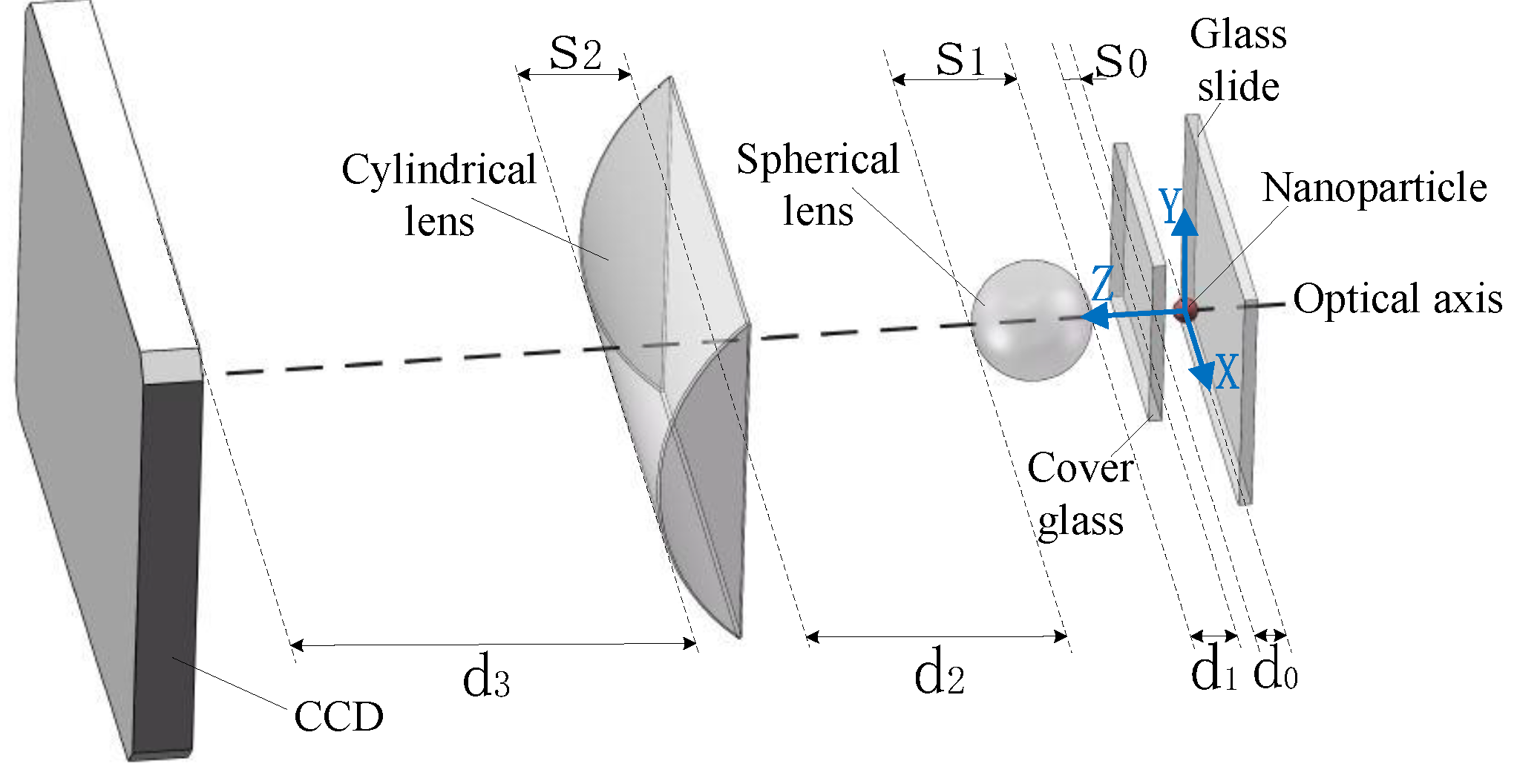
2. Micro-Imaging System

2.1. Ray Transfer Matrix of the Micro-Imaging System

Figure 1 presents the optical configuration of the proposed system and shows the components in the optical path. The Z-axis of the coordinate system coincides with the optical axis. d₀ is the distance between a cover glass and a single nanoparticle; and d₁, d₂, and d₃ are the distances between two optical components, which are unknown parameters; and s₀, s₁, and s₃ are the optical component thicknesses, as shown in Figure 1, which are the given parameters. Based on these parameters, the optical matrixes of the proposed system are as follows:

$$P_0=\left[\begin{array}{cccc}1& 0& {\mathrm{d}}_0& 0\\ 0& 1& 0& {\mathrm{d}}_0\\ 0& 0& 1& 0\\ 0& 0& 0& 1\end{array}\right], P_1=\left[\begin{array}{cccc}1& 0& {\mathrm{d}}_1& 0\\ 0& 1& 0& {\mathrm{d}}_1\\ 0& 0& 1& 0\\ 0& 0& 0& 1\end{array}\right], P_2=\left[\begin{array}{cccc}1& 0& {\mathrm{d}}_2& 0\\ 0& 1& 0& {\mathrm{d}}_2\\ 0& 0& 1& 0\\ 0& 0& 0& 1\end{array}\right],P_3=\left[\begin{array}{cccc}1& 0& {\mathrm{d}}_3& 0\\ 0& 1& 0& {\mathrm{d}}_3\\ 0& 0& 1& 0\\ 0& 0& 0& 1\end{array}\right],$$

$$L_0=\left[\begin{array}{cccc}1& 0& {\mathrm{n}}_{\mathrm{i}}{\mathrm{s}}_0/\mathrm{n}& 0\\ 0& 1& 0& {\mathrm{n}}_{\mathrm{i}}{\mathrm{s}}_0/\mathrm{n}\\ 0& 0& {\mathrm{n}}_{\mathrm{i}}/{\mathrm{n}}_{\mathrm{a}}& 0\\ 0& 0& 0& {\mathrm{n}}_{\mathrm{i}}/{\mathrm{n}}_{\mathrm{a}}\end{array}\right],$$

$$L_1=\left[\begin{array}{cccc}({\mathrm{n}}_{\mathrm{a}}-\mathrm{n})/\mathrm{n}& 0& {\mathrm{n}}_{\mathrm{a}}{\mathrm{s}}_1/\mathrm{n}& 0\\ 0& ({\mathrm{n}}_{\mathrm{a}}-\mathrm{n})/\mathrm{n}& 0& {\mathrm{n}}_{\mathrm{a}}{\mathrm{s}}_1/\mathrm{n}\\ 4{\mathrm{n}}_{\mathrm{a}}({\mathrm{n}}_{\mathrm{a}}-\mathrm{n})/({\mathrm{n}}_{\mathrm{a}}\mathrm{n}{\mathrm{s}}_1)& 0& ({\mathrm{n}}_{\mathrm{a}}-\mathrm{n})/\mathrm{n}& 0\\ 0& 4{\mathrm{n}}_{\mathrm{a}}({\mathrm{n}}_{\mathrm{a}}-\mathrm{n})/({\mathrm{n}}_{\mathrm{a}}\mathrm{n}{\mathrm{s}}_1)& 0& ({\mathrm{n}}_{\mathrm{a}}-\mathrm{n})/\mathrm{n}\end{array}\right],$$

$$L_2=\left[\begin{array}{cccc}1& 0& {\mathrm{n}}_{\mathrm{a}}{\mathrm{s}}_2/\mathrm{n}& 0\\ 0& 1& 0& {\mathrm{n}}_{\mathrm{a}}{\mathrm{s}}_2/\mathrm{n}\\ 0& 0& 1& 0\\ 0& ({\mathrm{n}}_{\mathrm{a}}-\mathrm{n})/({\mathrm{n}}_{\mathrm{a}}{\mathrm{R}}_{\mathrm{c}})& 0& (\mathrm{n}{\mathrm{R}}_{\mathrm{c}}+{\mathrm{s}}_2({\mathrm{n}}_{\mathrm{a}}-\mathrm{n}\left)\right)/(\mathrm{n}{\mathrm{R}}_{\mathrm{c}})\end{array}\right].$$

For the optical matrixes above, P₀, P₁, P₂, and P₃ are the transfer matrixes for propagation through the distances d₀, d₁, d₂, and d₃, respectively; and L₀, L₁, and L₂ are the transfer matrixes of the cover glass, spherical lens, and cylindrical lens, respectively. Here, R_c is the radius of curvature of the cylindrical lens, n_i, n_a, and n are the refractive indexes of the measured sample, air, and optical glass, respectively, all of which are given parameters. The integrated ray transfer matrix of this micro-imaging system is as follows:

$$W=P3\cdot L2\cdot P2\cdot L1\cdot P1\cdot L0\cdot P0=\left[\begin{array}{cccc}\mathrm{W}(1,1)& 0& \mathrm{W}(1,3)& 0\\ 0& \mathrm{W}(2,2)& 0& \mathrm{W}(2,4)\\ \mathrm{W}(3,1)& 0& \mathrm{W}(3,3)& 0\\ 0& \mathrm{W}(4,2)& 0& \mathrm{W}(4,4)\end{array}\right]$$

(1)

where W(row, col) indicates the parametric expression or constant value at row = row and column = col of the matrix W. Assuming the vector of a light ray from a point light source is X_e = [x_e, y_e, a_e, b_e]^T, where x_e and y_e are the X- and Y-axis coordinates, respectively, and a_e and b_e are the X- and Y-axis slopes of the corresponding ray, respectively, the corresponding vector of the light ray incident on the CCD is X_i = [x_i, y_i, a_i, b_i]^T = W·X_e.

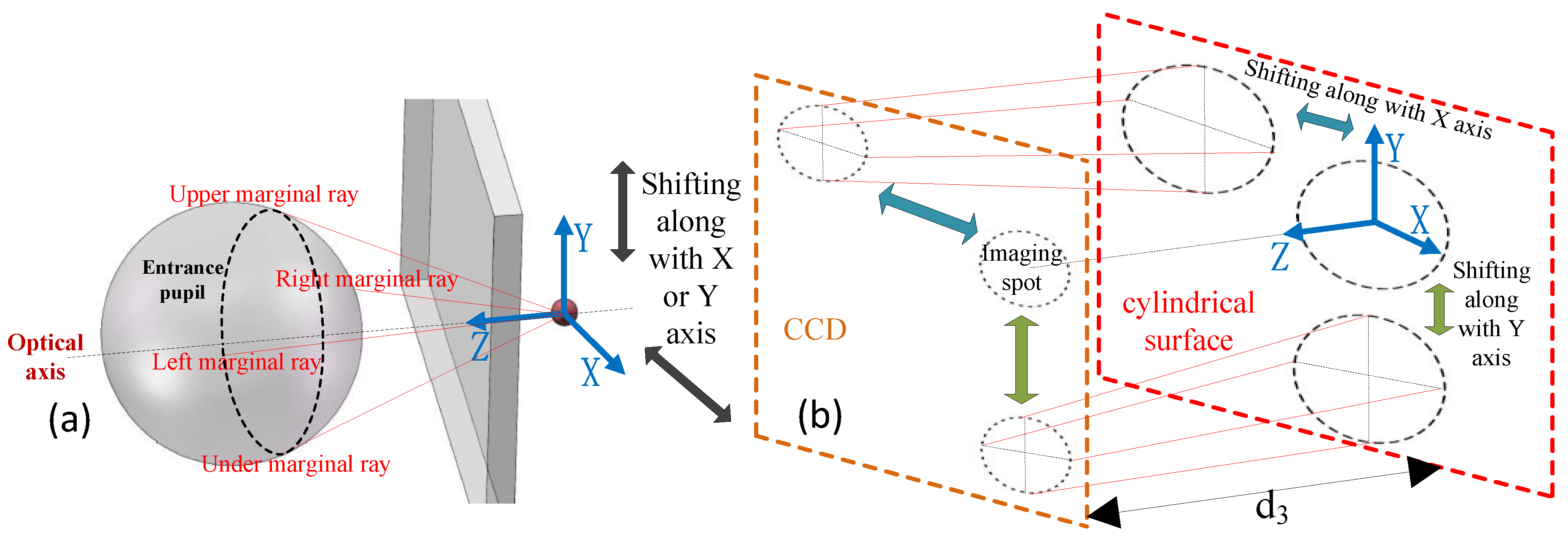
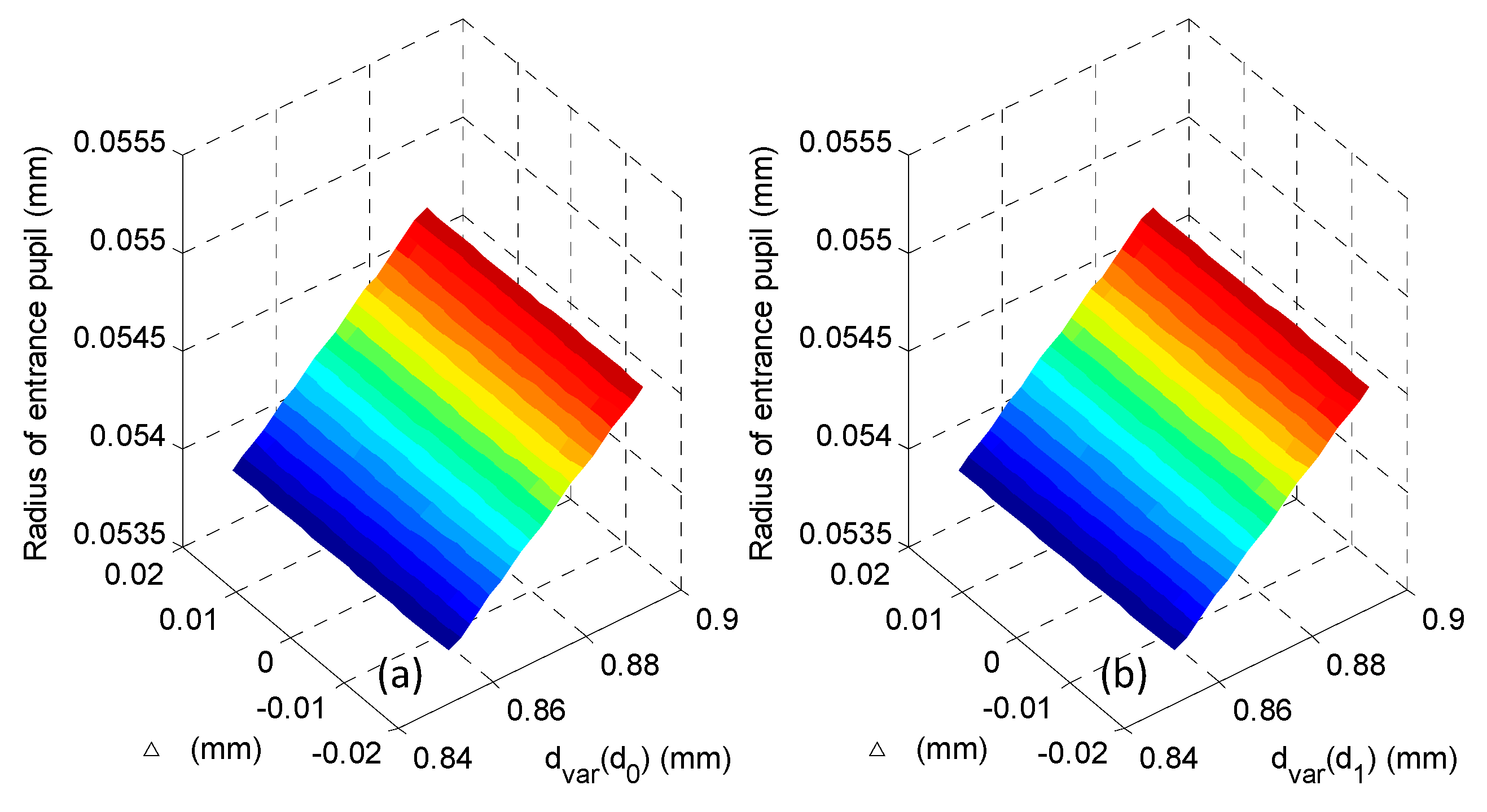
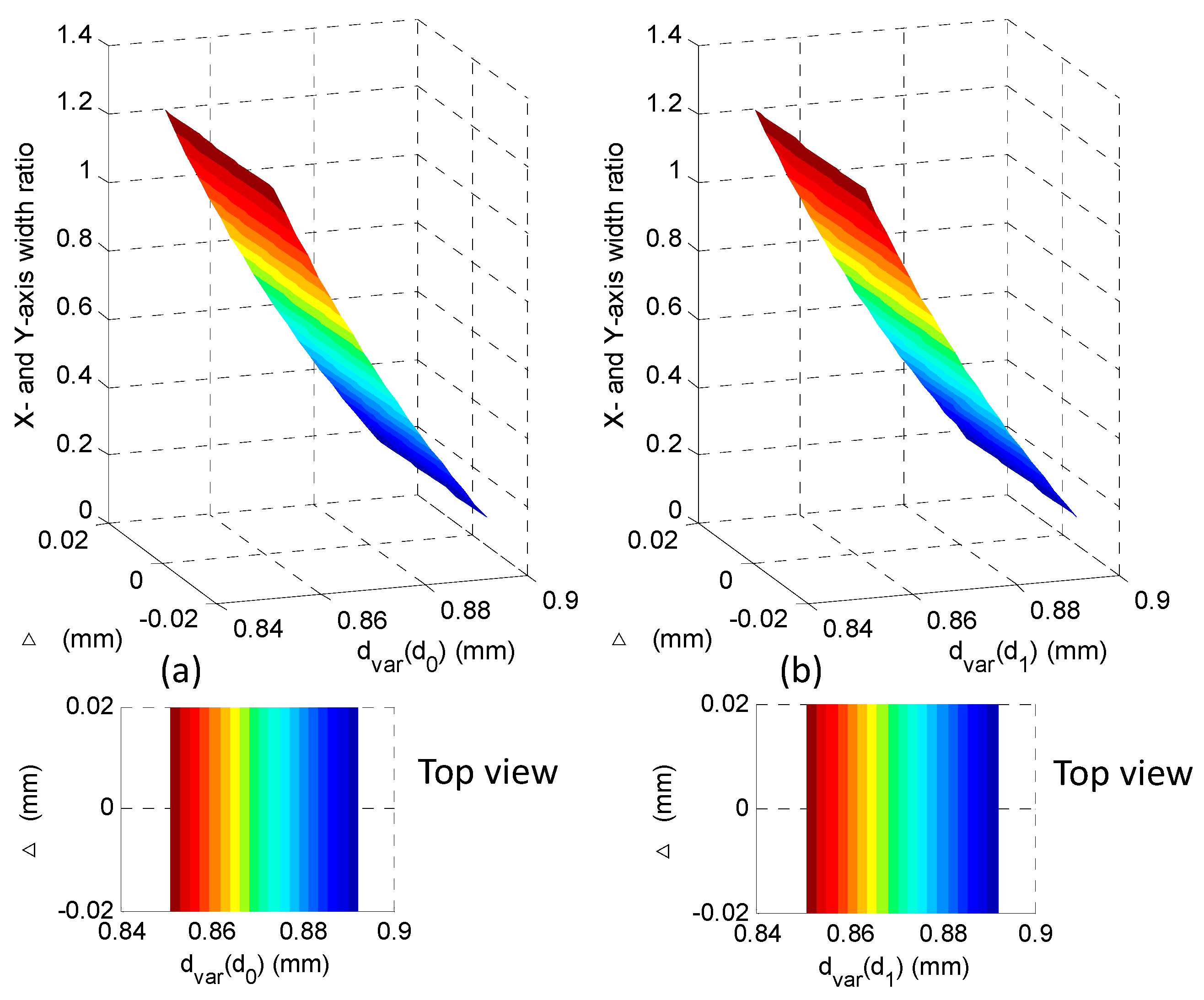
2.2. Analysis of the Micro-Imaging System

To realize an accurate measurement of the nanoparticle 3D trajectories with the micro-imaging system in Figure 1, there are two aspects that need to be analyzed: (1) analysis of whether the nanoparticle image intensity distributions corresponding to different coplanar positions on the same object plane are identical, and (2) analysis of the relationship between the coplanar displacements of the nanoparticle on the object plane and the corresponding coplanar displacements of the image on the image plane. The former is the requirement to realize an axial displacement measurement of the nanoparticle along the Z-axis, and the latter is the necessity to realize a coplanar displacement measurement of the nanoparticle in the XY plane.

The given parameters of the ray transfer matrix enumerated above are fixed values, except for n_i, which depends on the measured specimen. The unknown distance parameters are constant values for a particular magnification, except for d₀, which is the position of the nanoparticle fluorescent probe along the Z-axis. Initially, we determined the distance parameters d₁, d₂, and d₃ for analysis of the micro-imaging system.

To determine the distance parameters d₁, d₂, and d₃, each given parameter except n_i is assigned a value: n = 1.5, n_a = 1, R_c = 51.53 mm, s₀ = 0.17 mm, s₁ = 3 mm, and s₂ = 4.5 mm. If the emergent light ray is parallel to the Z-axis, namely, X_e = [x_e, y_e, 0, 0]^T, then −A_X = W(1, 1) = −1− 444.44 × d₂ − 444.44 × d₃ and −A_Y = W(2, 2) = −1− 434.74 × d₂ − 444.44 × (1 − 9.7 × d₃) × d₂, where −A_X and −A_Y are the magnifications along the X- and Y-axis, respectively. If the emergent light ray vector is X_e = [0, 0, a_e, b_e]^T, the corresponding incident light rays vector components x_i and y_i for ideal imaging are both zeros, no matter what the emergent light slopes a_e and b_e are. Thus, the equations 0 = W(1, 3) = −A_X × (d₀ + n_i × d₁) + 0.036 × n_i and 0 = W(2, 4) = −A_Y × (d₀ + n_i × d₁) + 0.025 × n_i should both be satisfied. Here, (d₀ + n_i × d₁) is denoted as d_var, where d_var = 0.025 × n_i/A_Y = 0.036 × n_i/A_X is the focal position on the optic axis at which a one-point light source can be ideally imaged. Making 0.025 × n_i/A_Y = 0.036 × n_i/A_X be true means the magnification ratio A_X/A_Y is 1.44; if the system is not capable of guaranteeing the magnification ratio, a one-point light source cannot be imaged to one point. For actual cases, the magnification ratio 1.44 is difficult to realize, and so a d_var variation range between 0.025 × n_i/A_Y and 0.036 × n_i/A_X is the relatively ideal focus depth. Obtaining d_var in the range means realizing the nanoparticle Z-axis position measurement for the micro-imaging system in Figure 1. Here, assuming −A_X = −53.67 and −A_Y = −39.07, then d₂ = 42 mm and d₃ = 76.5 mm; assuming n_i = 1.33, then 0.85 mm < d_var < 0.89 mm.

Before practically measuring the nanoparticle 3D trajectories, the imaging spot intensity distribution (X- and Y-axis width ratio) of the adopted nanoparticle probes when they are located on different longitudinal object planes should be calibrated. For nanoparticulate fluorescent probes, d₁ is constant and d₀ is varied to adjust d_var. Whereas, during calibration, because the adopted nanoparticle probe is fixed between the cover glass and the glass slide with fixative, d₀ is constant, and d_var varies with d₁. Therefore, when analyzing the two aspects of this micro-imaging system mentioned above, it is also necessary to verify whether the same d_var value has an identical influence on each of the two aspects. In addition, there are noises (e.g., Poisson noise and background noise) that affect the two aspects in an actual micro-imaging process, and so de-noising processing is needed, where there are many effective de-noising methods used to reduce the noises in actual measurements. Here, the effect of noises on micro-imaging is outside the scope of this study; analysis of the micro-imaging below is stated under the condition of non-noise, which does not contain the analysis of errors caused by noises.

The entrance pupil of one point on the fluorescent nanoparticle is determined by four marginal rays that are tangent to the spherical lens, as shown by Figure 2a. In Figure 2b, light exits from the cylindrical surface of the cylindrical lens. The width of the valid imaging spot along the X-axis is equal to the distance between the incident points of the right and left marginal rays, and the width along the Y-axis is equal to the distance between the incident points of the upper and lower marginal rays.

To ensure the established optical matrix of Equation (1) is modeled accurately, it requires surface size of the curved lens participating in micro-imaging to be significantly smaller than its radius of curvature, and this allows the lenses to be more accurately modeled in the paraxial approximation. In Figure 1, it is easy to make the cylindrical lens size far smaller than its radius of curvature, but the spherical lens size cannot meet the requirement. Obtaining a true nanoparticle image intensity distribution is not the desired outcome; rather, analyzing the two aspects stated above is our aim. The four marginal rays determining the angular aperture of the micro-imaging system can be used to analyze characters of the two aspects using the optical matrix of Equation (1); therefore, the rays determining the central part of the angular aperture also have the same function, namely the proportional variation of the angular aperture has no effect on the analysis of the two aspects. Reducing the angular aperture determined by the four marginal rays on each object plane with one same proportion is done to confirm the central part of the angular aperture, and to get four rays of the central angular aperture (namely, four central rays of the angular aperture) on each object plane. The scaled-down proportion can be chosen (here ten times is used), and the micro-imaging size of spherical lens determined by the four central rays is able to reach the requirement for running the optical matrix of Equation (1). The four central rays instead of original four marginal rays are used to implement the analysis with the optical matrix of Equation (1). The four marginal rays stated below are the four central rays.

According to diffraction theory, in the paraxial approximation, the image intensity distribution of a point light source is identical if the size of the entrance pupil (or the size of the exit pupil) remains the same. Figure 3 shows that irrespective of the distance Δ (along the X-axis or Y-axis) the point source (fluorescent nanoparticle) covers on an object plane, the size of the entrance pupil determined by the four central rays is constant, namely the nanoparticle image intensity distribution is constant for an object plane. The size changes with d_var, namely the nanoparticle image intensity distribution according to the object plane variation changes; furthermore, the presented sizes of the entrance pupil are identical for d_var during calibration and measurement as long as the values of d_var are the same. Thus, regarding the first aspect of analysis, it is proven that the nanoparticle imaging spot intensity distribution corresponding to different positions on same object plane do not vary for an object. For actual measurements, the entrance pupil size cannot be obtained; rather, what is obtained from the imaging plane is the X- and Y-axis width ratio of the point source imaging. Figure 4 shows that the X- and Y-axis width ratios of the point source imaging also changes with d_var, and so the X- and Y-axis width ratio can be used to mark different nanoparticle image intensity distributions along the Z-axis; thus, it can measure the nanoparticles displacement along the Z-axis.

To analyze the relationship between the coplanar displacement of the nanoparticle on the object plane and the corresponding coplanar displacement of the imaging spot on the image plane (the second aspect to be analyzed), it must first be determined how to calculate the center of the point source image.

When the point source is located on the Z-axis, the center of its image is at the intersection of the CCD and the Z-axis, which is also the intersection of the angular bisector of the right and left marginal rays (or upper and lower marginal rays) and the CCD. When a point source moves along the X-axis, the symmetrical relationship of the upper and lower marginal rays to the CCD in space is invariant, whereas the symmetrical relationship of the right and left marginal rays in space is undermined and the center of the image is shifted only along the X-axis, which is the intersection point between the angular bisector of the right and left marginal rays and the CCD. Similarly, for a point source moving along the Y-axis, the center of the image is the intersection point of the angular bisector of the upper and lower marginal rays and the CCD.

Figure 5 and Figure 6 show the center position measurement errors of the point source when it moves along the X (Δ_X) and Y (Δ_Y) axes, respectively. These figures show that the results are identical for d_var during measurement and calibration for the same value of d_var. The linear relationships between the measurement errors and the actual coplanar displacement of the point source are evident for different d_var’s. The slopes of the linear plane displacement measurement errors are also linearly related to d_var, as shown in Figure 7.

From the second requested analysis aspect stated above, the (fluorescent nanoparticle’s) actual coplanar displacement of the point source on an object plane can be related to its measured displacement value based on the linear relationship shown in Figure 7:

$$\begin{array}{l}\mathrm{actual}\mathrm{coplanar}\mathrm{displacement}\\ =\frac{\mathrm{measurement}\mathrm{coplanar}\mathrm{displacement}\mathrm{by}\mathrm{CCD}}{\left|\mathrm{magnification}\right|\cdot \left(1+\mathrm{slope}\mathrm{of}\mathrm{coplanar}\mathrm{displacement}\mathrm{measurement}\mathrm{error}\right)}\end{array}$$

(2)

The slope of the coplanar displacement measurement error differs with d_var, as seen in Figure 7; thus, the d_var measurement needs to be labeled when using Equation (2) to obtain the actual coplanar displacement. The d_var labeling process uses the longitudinal object planes calibration stated above.

3. Layout for Achieving Micro-Imaging

Figure 8 shows the configuration of the proposed micro-imaging system, where the fiber-coupled laser was mounted to the CCD and the ray emitted by the fiber-coupled laser was adjusted to be normal to the CCD using precision optical calibration and mechanical assembly. The emitted ray of the laser had a beam diameter of about 0.3 mm, and the glass block was attached to the cylindrical lens and objective stage. The optical surface of the glass block of the cylindrical lens was parallel to the flat surface of the cylindrical lens, and the optical surface of the glass block of the objective stage was parallel to the platform of the objective stage. A dual-spot position detection unit is a device for measuring the incident beam direction vector [26,27] and comprises two position-sensitive detectors (PSDs), several flat prisms, and a corner cube prism.

At first, the beam emitted by the fiber-coupled laser directly entered the dual-spot position detection unit, and the beam direction vector was obtained. The beam was then passed through the glass block of the cylindrical lens. The incident beam spot on two PSDs of the dual-spot position detection unit will be shifted if the glass block is not normal to the beam, namely the incidence angle θ_inc of the beam spot for the glass block is not zero, which is caused by pitch or yaw of the glass block.

$$\Lambda =\sin ({\theta }_{inc}-{\theta }_{ref})\cdot (h/\cos {\theta }_{ref})$$

(3)

Equation (3) is the relationship between the translation variation Λ of the beam spot on the two PSDs and θ_inc, where h is the thickness of the glass block and θ_ref is the refraction angle corresponding to θ_inc. It is easy to obtain θ_inc through Snell’s law sinθ_inc × n_a = sinθ_ref × n (where, n_a and n are the refractive indexes of air and glass, respectively) and Equation (3). After obtaining θ_inc, it is possible to adjust the cylindrical lens’ spatial attitude to make θ_inc be zero.

The coaxiality of the micro-imaging system is ensured by the above operation such that the magnification of the system can be confirmed. The beam was aligned such that it passes through the glass block of the cylindrical lens and was transmitted through the glass block of the objective table. Tilting the glass block of the objective stage such that its pitch and yaw were at a slight angle led to translation along the X- and Y-axes. These translations obtained by the dual-spot position detection unit were actual translations along the X- and Y-axes, and the values obtained by the CCD were the magnified translation variations along the X- and Y-axes. Therefore, the magnifications −A_X and −A_Y could be determined, and the d₂ and d₃ values corresponding to the obtained magnifications −A_X and −A_Y were easily calculated.

Here, there are two points to note: (1) to ensure that the object plane of the observed nanoparticle was normal to the optical axis of the micro-imaging system, the glass block of the objective stage must be normal to the beam, which was ensured in a similar way to the alignment of the glass block of the cylindrical lens; and (2) after the coaxiality and magnification calibration described above, a beam expander and deflection prism were inserted into the optical path after the beam exited from the dual-spot position detection unit, as shown in the lower right of Figure 8. The inserted beam expander and deflection prism were employed such that the expanded beam was incident sideways onto the sample to be measured sample to excite emission of the adopted fluorescent nanoparticle probe.

4. Experiments and Results

Except for the coaxiality and magnification calibration in Section 3, the operations to implement the d_var labeling process and to obtain the slope of coplanar displacement measurement error were also needed before the proposed micro-imaging system measured the 3D trajectory of the adopted fluorescent nanoparticle. In the operations, it was necessary to confirm the Z-axis and coplanar displacements of the adopted nanoparticle probe, which was fixed between the cover glass and glass slide. In Figure 8, the multidimensional displacement stage provided precise Z-axis and coplanar displacements for the operations.

Three fluorescent nanoparticles of diameters 50 nm, 100 nm, and 200 nm (fluorescence polystyrene, excitation peak: 540 nm, emission peak: 580 nm) were adopted. After being fixed between the cover glass and glass slide with the fixative (refractive index: 1.392), the d_var labeling process was implemented to build mapping relationships between the X- and Y-axis width ratios and the relative position along the Z-axis for the three fluorescent nanoparticles at three magnifications (M1: −A_X = −112.31 and −A_Y = −67.82; M2: −A_X = −53.67 and −A_Y = −39.07; M3: −A_X = −37.85 and −A_Y = −30.04), resulting in nine experiment results.

Figure 9a–c show the mapping relationships between the X- and Y-axis width ratios and the relative position along the Z-axis for fluorescent nanoparticles of three diameters, where the relative zero position was the position at which the width ratio was one for each case. Evidently, these mapping relationships could be used to obtain the Z-axis displacement of the three diameters of fluorescent nanoparticle in their actual measurement operations. After calibrating these mapping relationships, the relationships between the measurement errors and the actual coplanar displacement for each of the three diameters of fluorescent nanoparticles must be determined for realizing the coplanar displacement measurement according to Equation (2).

Figure 10a–f shows the relationship between the slope of the coplanar displacement measurement errors of five corresponding relative positions along the Z-axis for three diameters of a fluorescent nanoparticle. In Figure 10, the slopes corresponding to each of the five positions of each magnification can be seen to lie close to the fitted slope obtained by the micro-imaging system analysis. The intermediate magnification, M2, performed better than the other two magnifications, demonstrating that improper magnification has an influence on the measurement accuracy, where high magnification could cause noise to increase, and low magnification made the collected fluorescence nanoparticle images insufficiently accurate, both causing an inaccurate measurement. The degree of fit was used as a criterion to choose an appropriate magnification for the adopted fluorescent nanoparticle during the sample measurement.

After the above operations, the three fluorescent nanoparticles were dissolved in a silicone oil (refractive index: 1.392) to be the three test solutions. We synthesized the results of Figure 9 and Figure 10, and Equation (2) to realize the nine cases of the fluorescent nanoparticle 3D tracking measurements and to validate the performance of the proposed micro-imaging system. The diffusion constant D of the fluorescent nanoparticle had a relationship with its 3D MSD: MSD = 6Dt + σ, where σ was the offset at time zero, accounting for the positional accuracy, and t was the time delay. Figure 11 shows the relationships between the MSD in each case and the corresponding diffusion constant D.

Based on Stokes–Einstein theory, the diameter of a fluorescent nanoparticle can be estimated using the diffusion constant D, and the closer to the adopted standard diameter of fluorescent nanoparticle the estimated diameter is, the more correct the obtained diffusion constant D (the acquired MSD result) is [28]; the smaller the offset σ (the MSD error) is, the more correct the acquired MSD result is [24]. The accuracy of the diffusion constant D and the size of the offset σ both present how correct the acquired MSD result is. The correctness of the acquired MSD result can be confirmed by considering the overall performance of the diffusion constant D (accuracy of the estimated diameter) and the offset σ, where the influence of the diffusion constant D has a larger weight than the offset σ for judging the correctness of the acquired MSD result. The correctness of the acquired MSD result testifies to the measurement accuracy of the proposed imaging system.

Table 1. $\sigma$ of each case and diameter Ø of the fluorescent nanoparticle calculated using D.

Probe Ø	M1	M2	M3
50 nm	σ = 25.6 nm2, Ø = 43.6 nm	σ = − 12.1 nm2, Ø = 47.3 nm	σ = 69.4 nm2, Ø = 41.5 nm
100 nm	σ = 91.4 nm2, Ø = 81.8 nm	σ = 63.5 nm2, Ø = 102.8 nm	σ = −21.8 nm2, Ø = 67.1 nm
200 nm	σ = − 11.3 nm2, Ø = 174.3 nm	σ = 29.5 nm2, Ø = 192.1 nm	σ = 75.3 nm2, Ø = 154.8 nm

lists the σ of each magnification of each of the three diameters of fluorescent nanoparticle calculated using the respective diffusion constant. Evidently, the MSD error and calculated diameter corresponding to M2 were relatively small and exhibited the best agreement with the adopted fluorescent nanoparticles (particularly, for the case of measuring a 50 nm fluorescent nanoparticle). The selection of a magnification not corresponding to the adopted fluorescent nanoparticle will cause an inaccurate measurement; using a suitable magnification is important for fluorescent nanoparticle 3D tracking. The experiment proved the availability of the 3D zoom tracking of the adopted fluorescent nanoparticle with the proposed micro-imaging system.

5. Conclusions

In this paper, a 3D microscopic tracking system for single fluorescent nanoparticles based on astigmatic microscopic imaging was proposed, which principally involved a micro-imaging system comprising a spherical lens, a cylindrical lens, a CCD, and a dual-spot position detection unit. By analyzing the established ray transfer matrix of the proposed system and utilizing the beam vector measurement of the dual-spot position detection unit, it was demonstrated that the appropriate magnification of the adopted fluorescent nanoparticle could be selected to realize its accurate 3D tracking with the proposed system. The three diameters of the fluorescent nanoparticle were measured under three magnifications, and the tracking results for the intermediate magnification were the most accurate, which proved that the proposed tracking system could accurately track the adopted fluorescent nanoparticles in 3D through zoom microscopical measurements based on the self-calibration functions of coaxiality and magnification.

References

1. Cheng, L.C.; Hsiao, L.C.; Doyle, P.S. Multiple particle tracking study of thermally-gelling nanoemulsions. Soft Matter 2017, 13, 6606–6619. [Google Scholar] [CrossRef] [PubMed]
2. Zhang, Y.; Wei, C.; Lv, F.; Liu, T. Real-time imaging tracking of a dual-fluorescent drug delivery system based on doxorubicin-loaded globin-polyethylenimine nanoparticles for visible tumor therapy. Colloids Surf. B Biointerfaces 2018, 170, 163–171. [Google Scholar] [CrossRef]
3. Germann, J.A.; Davis, L.M. Three-dimensional tracking of a single fluorescent nanoparticle using four-focus excitation in a confocal microscope. Opt. Express 2014, 22, 5641–5650. [Google Scholar] [CrossRef] [PubMed]
4. Gross, A.; Torge, A.; Schaefer, U.F.; Schneider, M.; Lehr, C.-M.; Wagner, C. A foam model highlights the differences of the macro- and microrheology of respiratory horse mucus. J. Mech. Behav. Biomed. Mater. 2017, 71, 216–222. [Google Scholar] [CrossRef] [PubMed] [Green Version]
5. Kaur, G.; Lewis, J.S.; Oijen, A.M.V. Shining a Spotlight on DNA: Single-Molecule Methods to Visualise DNA. Molecules 2019, 24, 491. [Google Scholar] [CrossRef] [PubMed] [Green Version]
6. Nam, S.H.; Bae, Y.M.; Park, Y.I.; Kim, J.H.; Kim, H.M.; Choi, J.S.; Lee, K.T.; Hyeon, T.; Suh, Y.D. Long-TermReal-Time Tracking of Lanthanide Ion Doped Upconverting Nanoparticles in Living Cells. Angew. Chem. Int. Ed. 2011, 123, 6217–6221. [Google Scholar] [CrossRef]
7. Jo, H.L.; Song, Y.H.; Park, J.; Jo, E.-J.; Goh, Y.; Shin, K.; Kim, M.-G.; Lee, K.T. Fast and background-free three-dimensional (3D) live-cell imaging with lanthanide-doped upconverting nanoparticles. Nanoscale 2015, 7, 19397–19402. [Google Scholar] [CrossRef]
8. Goh, Y.; Song, Y.H.; Lee, G.; Bae, H.; Mahata, M.K.; Lee, K.T. Cellular uptake efficiency of nanoparticles investigated by three-dimensional imaging. Phys. Chem. Chem. Phys. 2018, 20, 11359–11368. [Google Scholar] [CrossRef]
9. Shin, K.; Song, Y.H.; Goh, Y.; Lee, K.T. Two-Dimensional and Three-Dimensional Single Particle Tracking of Upconverting Nanoparticles in Living Cells. Int. J. Mol. Sci. 2019, 20, 1424. [Google Scholar] [CrossRef] [Green Version]
10. Sio, S.D.; July, C.; Dhonta, J.K.G.; Lang, P.R. Near wall dynamics of a spherical particle in crowded suspensions of colloidal rods–dynamic information from TIRM revisited. Soft Matter 2018, 14, 9232–9242. [Google Scholar] [CrossRef] [Green Version]
11. Schoch, R.L.; Barel, I.; Brown, F.L.H.; Haran, G. Lipid diffusion in the distal and proximal leaflets of supported lipid bilayer membranes studied by single particle tracking. J. Chem. Phys. 2018, 148, 123333. [Google Scholar] [CrossRef] [PubMed]
12. Chen, K.; Gu, Y.; Sun, W.; Dong, B.; Wang, G.; Fan, X.; Xia, T.; Fang, N. Characteristic rotational behaviors of rod-shaped cargo revealed by automated five-dimensional single particle tracking. Nat. Commun. 2017, 8, 887. [Google Scholar] [CrossRef] [PubMed] [Green Version]
13. Cang, H.; Xu, C.S.; Montiel, D.; Yang, H. Guiding a confocal microscope by single fluorescent nanoparticles. Opt. Lett. 2007, 32, 2729–2731. [Google Scholar] [CrossRef] [PubMed]
14. Backlund, M.P.; Lew, M.D.; Backer, A.S. The role of molecular dipole orientation in single-molecule fluorescence microscopy and implications for super-resolution imaging. Chem. Phys. Chem. 2014, 15, 587–599. [Google Scholar] [CrossRef] [PubMed] [Green Version]
15. Schnitzbauer, J.; McGorty, R.; Huang, B. 4Pi fluorescence detection and 3D particle localization with a single objective. Opt. Express 2013, 21, 19701–19708. [Google Scholar] [CrossRef] [Green Version]
16. Gallatin, G.M.; Berglund, A.J. Optimal laser scan path for localizing a fluorescent particle in two or three dimensions. Opt. Express 2012, 20, 16381–16393. [Google Scholar] [CrossRef]
17. Adams, M.C.; Salmon, W.C.; Gupton, S.L.; Cohan, C.S.; Wittmann, T.; Prigozhina, N.; Waterman-storer, C.M. A high-speed multispectral spinning-disk confocal microscope system for fluorescent speckle microscopy of living cells. Methods 2003, 29, 29–41. [Google Scholar] [CrossRef]
18. Nakano, A. Spinning-disk confocal microscopy—A cutting-edge tool for imaging of membrane traffic. Cell Struct. Funct. 2002, 27, 349–355. [Google Scholar] [CrossRef] [Green Version]
19. Axelrod, D. Total Internal Reflection Fluorescence Microscopy in Cell Biology. Traffic 2001, 2, 764–774. [Google Scholar] [CrossRef]
20. Webb, R.H. Confocal optical microscopy. Rep. Prog. Phys. 1996, 59, 427–471. [Google Scholar] [CrossRef]
21. Schermelleh, L.; Carlton, P.M.; Haase, S.; Shao, L.; Winoto, L.; Kner, P.; Burke, B.; Cardoso, M.C.; Agard, D.A.; Gustafsson, M.G.L.; et al. Subdiffraction Multicolor Imaging of the Nuclear Periphery with 3D Structured Illumination Microscopy. Science 2008, 320, 1332–1337. [Google Scholar] [CrossRef] [PubMed] [Green Version]
22. Huisken, J.; Swoger, J.; Bene, F.D.; Wittbrodt, J.; Stelzer, E.H.K. Live Embryos by Selective Plane Illumination Microscopy. Science 2004, 305, 1007–1010. [Google Scholar] [CrossRef] [PubMed] [Green Version]
23. Kao, H.P.; Verkman, A.S. Tracking of single fluorescent particles in three dimensions: Use of cylindrical optics to encode particle position. Biophys. J. 1994, 67, 1291–1300. [Google Scholar] [CrossRef] [Green Version]
24. Holtzer, L.; Meckel, T.; Schmidt, T. Nanometric three-dimensional tracking of individual quantum dots in cells. Appl. Phys. Lett. 2007, 90, 053902. [Google Scholar] [CrossRef] [Green Version]
25. Pavani, S.R.; Thompson, M.A.; Biteen, J.S. Three-dimensional single-molecule fluorescence imaging beyond the diffraction limit by using a double-helix point spread function. Proc. Natl. Acad. Sci. USA 2009, 106, 2995–2999. [Google Scholar] [CrossRef] [PubMed] [Green Version]
26. Hu, P.; Mao, S.; Tan, J.B. Compensation of errors due to incident beam drift in a 3 DOF measurement system for linear guide motion. Opt. Express 2015, 23, 28389–28401. [Google Scholar] [CrossRef] [PubMed]
27. Mao, S.; Hu, P.; Ding, X.; Tan, J. Parameter correction method for dual position-sensitive-detector-based unit. Appl. Opt. 2016, 55, 4073–4078. [Google Scholar] [CrossRef]
28. Kato, H.; Ouchi, N.; Nakamura, A. Simultaneous measurement of size and density of spherical particles using two-dimensional particle tracking analysis method. Powder Technol. 2017, 315, 68–72. [Google Scholar] [CrossRef]
Figure 1. Optical configuration.
Applsci 10 00131 g001
Figure 2. Valid pupil area determined using a cone of light propagating from one point on the surface of a nanoparticle: (a) valid entrance pupil, and (b) corresponding valid exit pupil.
Applsci 10 00131 g002
Figure 3. Radius of the entrance pupil determined using the four central rays for different dvar and coplanar shift values Δ of the point source: (a) variation of dvar with d0, and (b) variation of dvar with d1.
Applsci 10 00131 g003
Figure 4. X- and Y-axis width ratios for different dvar and coplanar shift values Δ of the point source: (a) variation of dvar with d0, and (b) variation of dvar with d1.
Applsci 10 00131 g004
Figure 5. Measurement errors along the X-axis with different dvar values and actual shift value ΔX along the X-axis for a point source: (a) variation of dvar with d0, and (b) variation of dvar with d1.
Applsci 10 00131 g005
Figure 6. Measurement errors along the Y-axis with different dvar values and actual shift value ΔY along the Y-axis for a point source: (a) variation of dvar with d0, and (b) variation of dvar with d1.
Applsci 10 00131 g006
Figure 7. Slope of the coplanar displacement measurement error of the X-axis (a) and Y-axis (b).
Applsci 10 00131 g007
Figure 8. Schematic of the micro-imaging system with a dual-spot position detection unit.
Applsci 10 00131 g008
Figure 9. X- and Y-axis width ratio of three diameters of fluorescent nanoparticles versus their relative position, along with the Z-axis, at magnifications M1 (a), M2 (b), and M3 (c).
Applsci 10 00131 g009
Figure 10. Slopes of coplanar displacement measurement error of the X-axis (a) and Y-axis (b) for M1, X-axis (c) and Y-axis (d) for M2, and X-axis (e) and Y-axis (f) for M3, respectively.
Applsci 10 00131 g010
Figure 11. Relationships between each case of mean square displacement (MSD) and its corresponding diffusion constant D, for (a) M1, (b) M2, and (c) M3.
Applsci 10 00131 g011