Article

Individual Learning and Social Learning: Endogenous Division of Cognitive Labor in a Population of Co-evolving Problem-Solvers

by
Myong-Hun Chang
1,* and
Joseph E. Harrington, Jr.
2
1
Department of Economics, Cleveland State University, Cleveland, OH 44115, USA
2
Department of Business Economics and Public Policy, The Wharton School, University of Pennsylvania, Philadelphia, PA 19102, USA
*
Author to whom correspondence should be addressed.
Adm. Sci. 2013, 3(3), 53-75; https://doi.org/10.3390/admsci3030053
Submission received: 17 May 2013 / Revised: 28 June 2013 / Accepted: 2 July 2013 / Published: 12 July 2013
(This article belongs to the Special Issue Computational Organization Theory)

Abstract

:
The dynamic choice between individual and social learning is explored for a population of autonomous agents whose objective is to find solutions to a stream of related problems. The probability that an agent is in the individual learning mode, as opposed to the social learning mode, evolves over time through reinforcement learning. Furthermore, the communication network of an agent is also endogenous. Our main finding is that when agents are sufficiently effective at social learning, structure emerges in the form of specialization. Some agents focus on coming up with new ideas while the remainder of the population focuses on imitating worthwhile ideas.

“Innovate. That’s what we do.”
—Steve Jobs during his keynote speech for Apple Expo in Paris, 16 September 2003 [1].
“These guys can be taken but the only way we are going to take them is by studying them, know what they know, do what they do, watch them, watch them, watch them, look for every angle, stay on their shoulders, clone them, take every one of their good ideas and make it one of our good ideas.”
—Steve Ballmer of Microsoft in pep rally footage in the mid 1990’s [2].

1. Introduction

As a firm’s competitors alter their products and consumers’ preferences evolve, it may become necessary for the firm to introduce new products or update a product design. This often involves discovering consumer preferences for various product attributes as they evolve over time. Such a discovery process may involve an individualistic learning mechanism such as innovation or a social and interactive one such as imitation. The academic community is no different from the marketplace in this regard. A scientist’s search for the solution to a major scientific problem is driven by both the individual and social learning processes in which progress is made through exploration by oneself and exploitation of discoveries made by others:
Sometimes scientists modify their cognitive states as results of asocial interactions, sometimes they change their minds through social exchanges. The obvious exemplars for the former are the solitary experimentalist at work with apparatus and samples and the lone field observer attending to the organisms—although I shall also take encounters with nature to cover those occasions on which scientists reflect, constructing chains of reasoning that modify their commitments. Paradigm cases of conversations with peers are those episodes in which one scientist is told something by another (and believe it) or when a change in commitment is caused by the reading of a text. The point of the distinction is evidently to separate those episodes that (very roughly) consist in finding things out for oneself from those in which one relies on others.
[Kitcher [3]:60]
Whether the participants in the search process are motivated by profits or the recognition of the peers, the specific learning mechanisms used by the individuals and how these mechanisms mutually interact with one another can influence the growth in the stock of knowledge that is available for all participants. Our objective in this paper is to investigate how the individual choices of learning mechanisms coevolve in such a setting where the social aspect of the learning process is a prominent feature.
We employ a computational model which entails a population of autonomous agents whose objective is to find solutions to a stream of possibly related problems arriving over time. An individual’s search for solutions is driven by her choice of a learning mechanism each period. We consider two distinct learning mechanisms—individual learning (innovation) and social learning (imitation). The choice between the two learning modes is probabilistic, where the probability of choosing a given mode is adjusted over time by each agent on the basis of reinforcement learning. The agents are homogeneous in terms of their innate abilities to engage in the two modes of learning. They also operate in identical environments and face the same series of problems: The population may be most usefully considered as that of the members of a single organization who work toward a common goal in a shared environment. In this setting, we examine the long-run time paths of the endogenous probabilities with which the agents choose the two learning mechanisms.
Individual learning entails the solitary act of exploration, through which an agent comes upon a serendipitous discovery of her own without any external influence. In contrast, social learning relies strictly on the agent’s social network, whereby another agent in the network is selected for observation and an idea of hers is considered for direct copying. The structure of each agent’s social network—in terms of the probabilities with which a given agent observes all other agents—evolves over time on the basis of how effective it has been in facilitating the search for the solution. The coevolving social networks of all agents in the population then determine the relative benefits to individual agents of using one or the other of the two alternative learning mechanisms, which, in turn, guide the evolution of the choice probabilities through reinforcement learning.
In that the model of this paper is closely related to the one in Chang and Harrington [4], let us summarize that paper so as to better convey the contribution of this paper. The objective of Chang and Harrington [4] was to characterize network structure and population performance and explore their dependence on the reliability of the communications technology, as well as the innovativeness of agents. When the communications technology is poor, it was found, not surprisingly, that technological improvements enhance performance. What was surprising is that if the communications technology is sufficiently effective, further improvements are detrimental. Better communications allows more social learning among agents and this endogenously results in a more structured network as each agent is able to identify those agents from which she can learn. (As agents faced different environments, an agent wants to connect with those agents who face similar environments and thus are likely to have applicable solutions.) This, however, has the unfortunate by-product that it results in agents having very similar solutions and the ensuing lack of diversity within the social network meant that the population of agents is ill-equipped to adapt to a changing environment. Thus, a better communications technology can lead to too structured a network from the perspective of promoting innovation.
The contribution of the current paper concerns a different facet to structure. The focus is not on the network but rather the different roles that agents play in the population. In contrast to Chang and Harrington [4], all agents are assumed to face the same environment but, as in that paper, agents are equally skilled. Thus, in all respects, agents are ex ante identical. [Variants of this model when agents have heterogeneous skills with respect to individual learning and social learning are analyzed in Chang and Harrington [5] and Chang [6].] The main result in this paper is that, in spite of the homogeneity of agents, behavioral diversity arises and persists over time. As the efficacy of social learning rises relative to that of individual learning, we naturally find that agents engage in relatively more social learning. What is striking is that structure to the population emerges as there is a move towards specialization; some agents focus more on individual learning and others focus more on social learning. This emergent structure is also found to be stronger when agents are more skilled (in both social and individual learning) and when the environment is more stable. This finding leads to an alternative interpretation of an empirical observation. If one were to observe some agents in the population generating more new ideas, it need not be due to those agents being more original and insightful but rather that they have decided to devote more effort to individual learning.
The next section describes the model in detail. In Section 3, we describe the design of the computational experiments as well as the parameter values used in these experiments. Results are derived for small populations—two or three agents—in Section 4. Section 5 considers larger populations and shows that the findings for small populations are robust. Section 6 concludes.

2. The Model

2.1. Agents, Tasks, Goal and Performance

The population consists of L individuals. Each individual i { 1 , 2 , , L } engages in an operation (solving of a problem) which can be broken down into H separate tasks. There are several different methods which can be used to perform each task. The method chosen by an agent for a given task is represented by a sequence of d bits (0 or 1) such that there are 2 d possible methods available for each task. In any period t, an individual i is then fully characterized by a binary vector of H · d dimensions, which can be interpreted as his “approach” to solving an existing problem. Denote it by z ̲ i ( t ) { 0 , 1 } H d so that z ̲ i ( t ) ( z ̲ i 1 ( t ) , . . . , z ̲ i H ( t ) ) and z ̲ i h ( t ) ( z i h , 1 ( t ) , . . . , z i h , d ( t ) ) { 0 , 1 } d is individual i’s chosen method in task h { 1 , . . . , H } .
The degree of heterogeneity between two methods vectors, z ̲ i and z ̲ j , is measured using “Hamming distance” which is defined as the number of positions for which the corresponding bits differ:
D ( z ̲ i , z ̲ j ) h = 1 H k = 1 d z i h , k z j h , k
In period t, the population faces a common goal vector, z ̲ ^ ( t ) { 0 , 1 } H d . The goal vector is uniquely specified for the problem the population is faced with in period t and represents the approach which is optimal for solving it. It may be useful to recall Kuhn’s [7] treatment of “normal science as puzzle-solving” in which a scientific theory is an instrument for discovering and solving puzzles. The “goal” vector in our model is the method (instrument) best suited for solving the problem in hand. The perpetual search for such a goal is what gives rise to scientific progress in our framework. Our perspective is then consistent with Kuhn’s notion of scientific progress as elaborated in his Postscript written in 1969: “I do not doubt, for example, that Newton’s mechanics improves on Aristotle’s and that Einstein’s improves on Newton’s as instruments for puzzle-solving.” [Kuhn [7]: 206]
In our model, the population faces a stream of related problems, one for each period, such that the optimal approach for solving the problem can change from one period to the next. The degree of turbulence in the problem environment is then captured by intertemporal variability in z ̲ ^ ( t ) , the details of which are to be explained in 2.4.
The individuals are uninformed about z ̲ ^ ( t ) ex ante, but engage in “search” to get as close to it as possible. Given H tasks with d bits in each task and the goal vector z ^ ( t ) , the period-t performance of individual i is then measured by π i ( t ) , where
π i ( t ) = H · d D ( z ̲ i ( t ) , z ^ ̲ ( t ) )

2.2. Modeling Individual and Social Learning

In a given period, an individual’s search for the current optimum is carried out through two distinct modes, individual learning and social learning. Individual learning is when an individual independently discovers and considers for implementation a random method for a randomly chosen task. Social learning is when an individual selects someone and then observes and considers implementing the method currently deployed by that agent for one randomly chosen task.
Although each act of individual or social learning is assumed to be of a single task, this is without loss of generality: If we choose to define a task as including d dimensions, the case of a single act of individual or social learning involving two tasks can be handled by setting d = 2 d . [There is a restriction in that an agent only has the option of adopting all d dimensions or none.] In essence, what we are calling a “task” is defined as the unit of discovery or observation. The actual substantive condition is instead the relationship between d and H, as an agent’s individual or social learning involves a smaller part of the possible solution when d / H is smaller.
Whether obtained through individual or social learning, an experimental method is actually adopted if and only if its adoption brings the agent closer to the goal by decreasing the Hamming distance between the agent’s new methods vector and the goal vector.

2.3. Endogenizing Choices for Individual and Social Learning

We assume that in each period an individual may engage in either individual learning or social learning by using the network. How exactly does an individual choose between these learning modes and, if he chooses to engage in social learning, how does he decide from whom to learn? We model this as a two-stage stochastic decision process with reinforcement learning. The description of the model in this section is identical to that in Chang and Harrington [4].
Figure 1. Decision sequence of individual i in period t.
Admsci 03 00053 g001
Figure 1 describes the timing of decisions in our model. In stage 1 of period t, individual i is in possession of the current methods vector, z ̲ i ( t ) , and chooses individual learning with probability q i ( t ) and social learning with probability 1 q i ( t ) . If he chooses individual learning then, with probability μ i I , he generates an idea which is a randomly chosen task h { 1 , , H } and a randomly chosen method, z ̲ i h , for that task such that the experimental method vector is z ̲ i ( t ) ( z ̲ i 1 ( t ) , , z ̲ i h 1 , z ̲ i h , z ̲ i h + 1 , , z ̲ i H ( t ) ) . μ i I is a parameter that controls the inherent ability of an agent to engage in individual learning. This experimental vector is adopted by i if and only if its adoption decreases the Hamming distance between the agent and the current goal vector, z ̲ ^ ( t ) . Otherwise, it is discarded:
z ̲ i ( t + 1 ) = { z ̲ i , if  D ( z ̲ i , z ̲ ^ ( t ) ) < D ( z ̲ i , z ̲ ^ ( t ) ) z ̲ i , if  D ( z ̲ i , z ̲ ^ ( t ) ) D ( z ̲ i , z ̲ ^ ( t ) )
Alternatively, with probability 1 μ i I the individual fails to generate an idea, in which case z ̲ i ( t + 1 ) = z ̲ i ( t ) .
Now suppose individual i chooses to engage in social learning in stage 1. Given that he decides to learn from someone else, he taps into the network to make an observation. Tapping into the network is also a probabilistic event, in which with probability μ i S the agent is connected to the network, while with probability 1 μ i S the agent fails to connect. Hence, μ i S measures the ability of the agent to communicate with others in the population. An agent that is connected then enters stage 2 of the decision process in which he must select another agent to observe. Let p i j ( t ) be the probability with which i observes j in period t so j i p i j ( t ) = 1 for all i. If agent i observes another agent l, that observation involves a randomly chosen task h and the current method used by agent l in that task, z ̲ l h ( t ) . Let z ̲ i ( t ) = ( z ̲ i 1 ( t ) , , z ̲ i h 1 ( t ) , z ̲ l h ( t ) , z ̲ i h + 1 ( t ) , , z ̲ i H ( t ) ) be the experimental vector. Adoption or rejection of the observed method is based on the Hamming distance criterion:
z ̲ i ( t + 1 ) = { z ̲ i , if  D ( z ̲ i , z ̲ ^ ( t ) ) < D ( z ̲ i , z ̲ ^ ( t ) ) z ̲ i , if  D ( z ̲ i , z ̲ ^ ( t ) ) D ( z ̲ i , z ̲ ^ ( t ) )
If the agent fails to connect to the network, which occurs with probability 1 μ i S , z ̲ i ( t + 1 ) = z ̲ i ( t ) .
The probabilities, q i ( t ) and { p i 1 ( t ) , , p i i 1 ( t ) , p i i + 1 ( t ) , , p i L ( t ) } , are adjusted over time by individual agents according to a reinforcement learning rule. We adopt a version of the Experience-Weighted Attraction (EWA) learning rule as described in Camerer and Ho [8]. Using this rule, q i ( t ) is adjusted each period on the basis of evolving attraction measures, A i I ( t ) for individual learning and A i S ( t ) for social learning. The evolution of A i I ( t ) and A i S ( t ) follow the process below:
A i I ( t + 1 ) = { ϕ A i I ( t ) + 1 , if  i  adopted a method through individual learning in  t ϕ A i I ( t ) , otherwise ;
A i S ( t + 1 ) = { ϕ A i S ( t ) + 1 , if  i  adopted a method through social learning in  t ϕ A i S ( t ) , otherwise ;
where ϕ ( 0 , 1 ] . Hence, if the agent chose to pursue individual learning and discovered and then adopted his new idea, the attraction measure for individual learning increases by 1 after allowing for the decay factor of ϕ on the previous attraction level. If the agent chose individual learning but was unsuccessful (either because he failed to generate an idea, or because the idea he generated was not useful) or if he instead chose social learning, then his attraction measure for individual learning is simply the attraction level from the previous period decayed by the factor ϕ. Similarly, a success or failure in social learning at t has the identical influence on A i S ( t + 1 ) . Given A i I ( t ) and A i S ( t ) , one derives the choice probability of individual learning in period t as follows:
q i ( t ) = A i I ( t ) λ A i I ( t ) λ + A i S ( t ) λ
where λ > 0 . A high value of λ means that a single success has more of an impact on the likelihood of repeating that activity (individual or social learning). The probability of pursuing social learning is, of course, 1 q i ( t ) . The expression in (7) says that a favorable experience through individual learning (social learning) raises the probability that an agent will choose individual learning (social learning) again in the future. In sum, a positive outcome realized from a course of action reinforces the likelihood of that same action being chosen again. For analytical simplicity, we assume ϕ and λ to be common to all individuals in the population.
The stage-2 attractions and the probabilities are derived similarly. Let B i j ( t ) be agent i’s attraction to another agent j in period t. It evolves according to the rule below:
B i j ( t + 1 ) = { ϕ B i j ( t ) + 1 , if  i  successfully learned from  j  in  t ϕ B i j ( t ) , otherwise
j i . The probability that agent i observes agent j in period t is adjusted each period on the basis of the attraction measures, { B i j ( t ) } j i :
p i j ( t ) = B i j ( t ) λ h i B i h ( t ) λ
j i , i , where λ > 0 .
There are two distinct sets of probabilities in our model. One set of probabilities, q i ( t ) and { p i j ( t ) } j i , are endogenously derived and evolve over time in response to the personal experiences of agent i. Another set of probabilities, μ i I and μ i S , are exogenously specified and are imposed on the model as parameters. They control the capabilities of individual agents to independently learn or to learn from someone else in the population via social learning. It is particularly interesting to understand how these parameters influence the evolution of the probabilities with which the agents choose a given learning mechanism.

2.4. Modeling Turbulence in Task Environment

Central to the performance of a population is how it responds to an evolving environment or, if we cast this in the context of problem-solving, an evolving set of problems to be solved. It is such change that makes individual learning and the spread through a social network of what was learned so essential. Change or turbulence is specified in our model by first assigning an initial goal vector, z ^ ( 0 ) , to the population and then specifying a dynamic process by which it shifts over time.
Letting s { 0 , 1 } H d , define δ ( s , κ ) { 0 , 1 } H d as the set of points that are exactly Hamming distance κ away from s. The set of points within Hamming distance κ of s is defined as
Δ ( s , κ ) i = 0 κ δ ( s , i )
Hence, Δ ( s , κ ) is a set whose “center” is s.
In period t, all agents in the population have the common goal vector of z ^ ̲ ( t ) . In period t + 1 , the goal stays the same with probability σ and changes with probability ( 1 σ ) . The shift dynamic of the goal vector is guided by the following stochastic process. The goal in t + 1 , if different from z ^ ̲ ( t ) , is then an i i d selection from the set of points that lie within the Hamming distance ρ of z ^ ̲ ( t ) . Defining Λ ( z ^ ̲ ( t ) , ρ ) as the set of points from which the goal in t + 1 is chosen, we have
Λ ( z ^ ̲ ( t ) , ρ ) Δ ( z ^ ̲ ( t ) , ρ ) \ z ^ ̲ ( t )
Hence, Λ ( z ^ ̲ ( t ) , ρ ) includes all points in Δ ( z ^ ̲ ( t ) , ρ ) except for z ^ ̲ ( t ) . Consequently,
z ^ ̲ ( t + 1 ) = z ^ ̲ ( t ) with probability σ z ^ ̲ ( t + 1 ) Λ ( z ^ ( t ) , ρ ) with probability 1 σ
The goal vector for the population then stochastically fluctuates while remaining within Hamming distance ρ of the current goal. This allows us to control the possible size of the inter-temporal change. The lower is σ and the greater is ρ, the more frequent and variable is the change, respectively, in the population’s goal vector.

3. Design of Computational Experiments

The underlying simulation model specifies H = 24 and d = 4 , so that there are 96 total bits in a methods vector and over 7 . 9 × 10 28 possibilities in the search space.
We consider a variety of population sizes: L { 2 , 3 , 5 , 10 , 20 , 50 } . While the agents are homogeneous in their skills for individual and social learning, i.e., ( μ i I , μ i S ) = ( μ I , μ S ) i , we are interested in how the levels of μ I and μ S affect the endogenous choice probabilities. As such, we consider various combinations of values for ( μ I , μ S ) , where μ I { 0 . 1 , 0 . 2 , . . . , 1 } and μ S { 0 . 1 , 0 . 2 , . . . , 1 } .
We assume that the initial practices of the agents are completely homogeneous so that z _ i ( 0 ) = z _ j ( 0 ) i j . This is to ensure that any social learning occurring over the horizon under study entails only newly generated knowledge. Otherwise, the initial variation in the information levels of the agents will induce some social learning, introducing unnecessary random noise into the system. The common initial methods vector is assumed to be an independent draw from { 0 , 1 } H d .
The impact of environmental volatility is explored by considering values of σ from { 0 . 5 , 0 . 6 , 0 . 7 , 0 . 8 , 0 . 9 } and ρ from { 1 , 2 , 4 , 6 , 9 } .
Additional parameters are ϕ and λ, which control the evolution of the attraction measures. For simplicity, we assume that ϕ = 1 and λ = 1 throughout the paper. Finally, the initial attraction stocks are set at B i j ( 0 ) = 1 i , j i , and A i I ( 0 ) = A i S ( 0 ) = 1 i . Hence, an individual is initially equally attracted to individual and social learning and has no inclination to observe one individual over another ex ante.
All computational experiments carried out here assume a horizon of 15,000 periods. The time-series of the performance measures are observed to reach a steady-state by the 2,000th period. We measure the steady-state performance of individual i, denoted π ¯ i , to be the average over the last 5,000 periods of this horizon such that
π ¯ i = 1 5 , 000 t = 10 , 001 15 , 000 π i ( t )
The mean steady-state performance of the population is then denoted:
π ¯ 1 L i = 1 L π ¯ i
Likewise, the endogenous steady-state probability of individual learning, denoted q ¯ i , is computed for each agent as the average over the last 5,000 periods:
q ¯ i = 1 5 , 000 t = 10 , 001 15 , 000 q i ( t )
The steady-state probability of social learning for agent i is then 1 q ¯ i .
All of the experiments were based on 100 replications, each using a fresh set of random numbers. Hence, the model is run for 1.5 million periods for each parameter configuration considered in this paper. The performance and probability measures reported in the paper are the averages of those 100 replications.

4. Learning in Small Populations

We first consider “small” populations by which is meant those with two or three agents. The reason for initially focusing on these cases is that the vector of probabilities (of an agent being in the individual learning mode) can be depicted graphically which quite effectively illustrates what is going on. In the next section, larger populations are considered and, using different methods for reporting results, we show that much of the insight of this section extends. Note that, with only two agents, each agent has only one other agent to observe when she chooses social learning so the structure of the social network is not an issue. The endogeneity of the network is an issue, however, when there are three agents. Procedurally, we will first report results for when there are two agents and then show that the same property holds for when there are three agents.

4.1. Emergence of Specialization

To establish a baseline for comparative analyses, we ran the computational experiment with the following set of parameter values: μ I = μ S = 1 . 0 , σ = 0 . 8 , and ρ = 1 . Both agents are capable of generating an idea every period, whether it is through individual learning or through social learning. There is a probability of 0.8 that the problem environment will be stable from t to t + 1 . If the environment changes, which occurs with the probability of 0.2, it involves a change in only one randomly chosen task.
The two agents are initially homogeneous in all aspects. They have identical levels of skills in individual and social learning so that μ 1 I = μ 2 I μ I = 1 . 0 and μ 1 S = μ 2 S μ S = 1 . 0 . They start out equally likely to choose individual learning and social learning so that q 1 ( 0 ) = q 2 ( 0 ) = 0 . 5 .
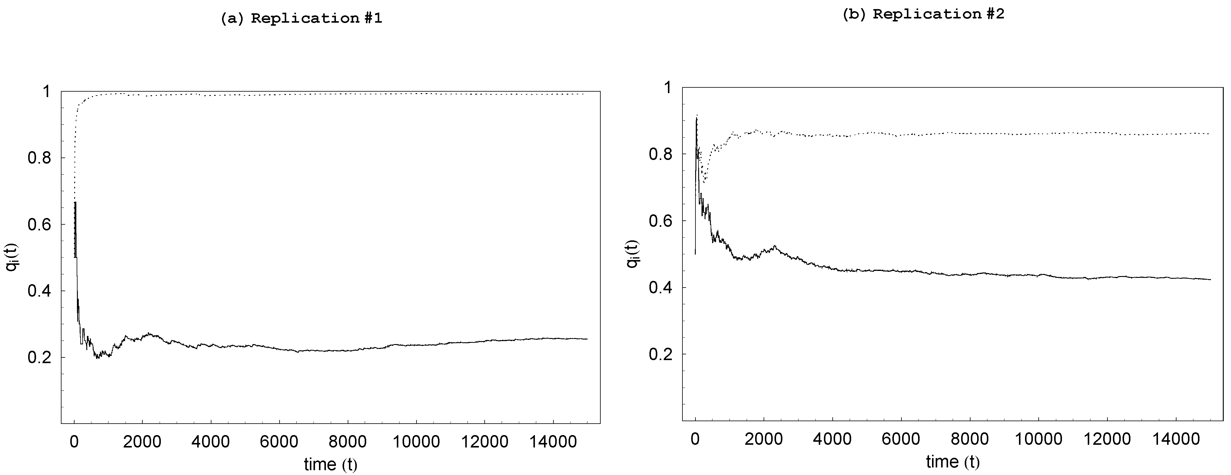
Given the baseline parameter configuration, Figure 2 shows the typical time paths of q i ( t ) s for i { 1 , 2 } which are generated from two independent replications. The time paths captured in these figures, which are typical of all replications carried out in this work, clearly indicate that our definition of the steady-state as the 5,000 period between t = 10 , 001 and t = 15 , 000 is more than adequate: While there is a brief initial transient phase in which q i ( t ) s fluctuate somewhat widely, they tend to stabilize rather quickly. It is clear that these probabilities exhibit high degrees of persistence. What is more striking, however, is the way q i ( t ) s diverge from one another in the long run: the agents tend to concentrate on distinct learning mechanisms—agent i specializing in individual learning (high value of q i ( t ) ) and agent j specializing in social learning (low value of q j ( t ) ) and, thus, free-riding on agent i for knowledge acquisition.
Figure 2. Typical time paths of q i ( t ) s from two replications ( μ I = μ S = 1 . 0 , σ = 0 . 8 , and ρ = 1 ).
Admsci 03 00053 g002
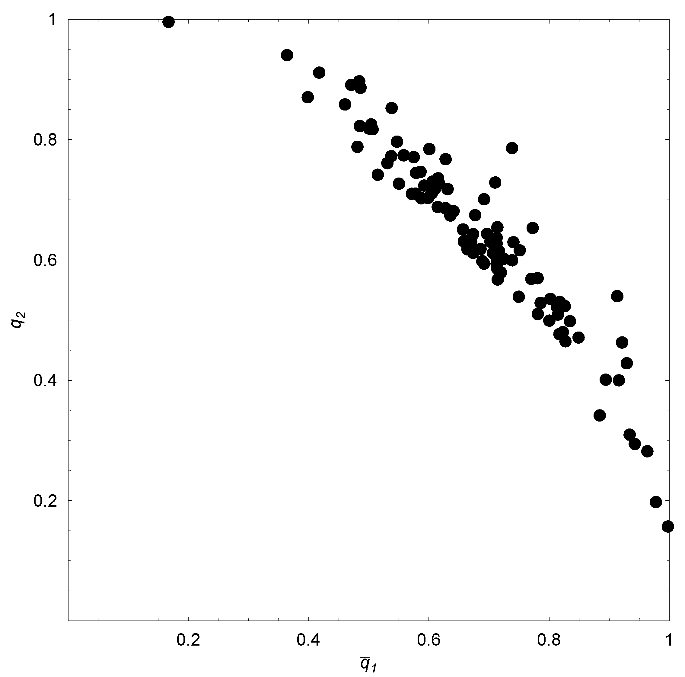
To confirm the tendency for the agents to specialize, we ran 100 replications for the baseline set of parameter values, each replication with a fresh set of random numbers. The steady-state probabilities for the two agents, q ¯ 1 and q ¯ 2 , were then computed for each replication, thereby giving us 100 realizations of the probability pair. In Figure 3, these realizations are plotted in a probability space. Note the strongly negative correlation between q ¯ 1 and q ¯ 2 . More intensive individual (social) learning by an agent induces the other agent to pursue more intensive social (individual) learning. As this property is confirmed by results reported below for other parameter configurations and when there are three agents, we state:
Property 1 For populations with two or three agents, there emerges a divergence in the choices of learning modes: When one agent chooses individual learning with a higher probability, the other agent(s) chooses social learning with a higher probability.
The implication is that social learners free-ride on an individual learner and an individual learner accommodates such behavior by concentrating on generating new ideas.
Figure 3. ( q ¯ 1 , q ¯ 2 )’s with μ I = μ S = 1 . 0 over 100 replications ( σ = 0 . 8 , ρ = 1 ).
Admsci 03 00053 g003
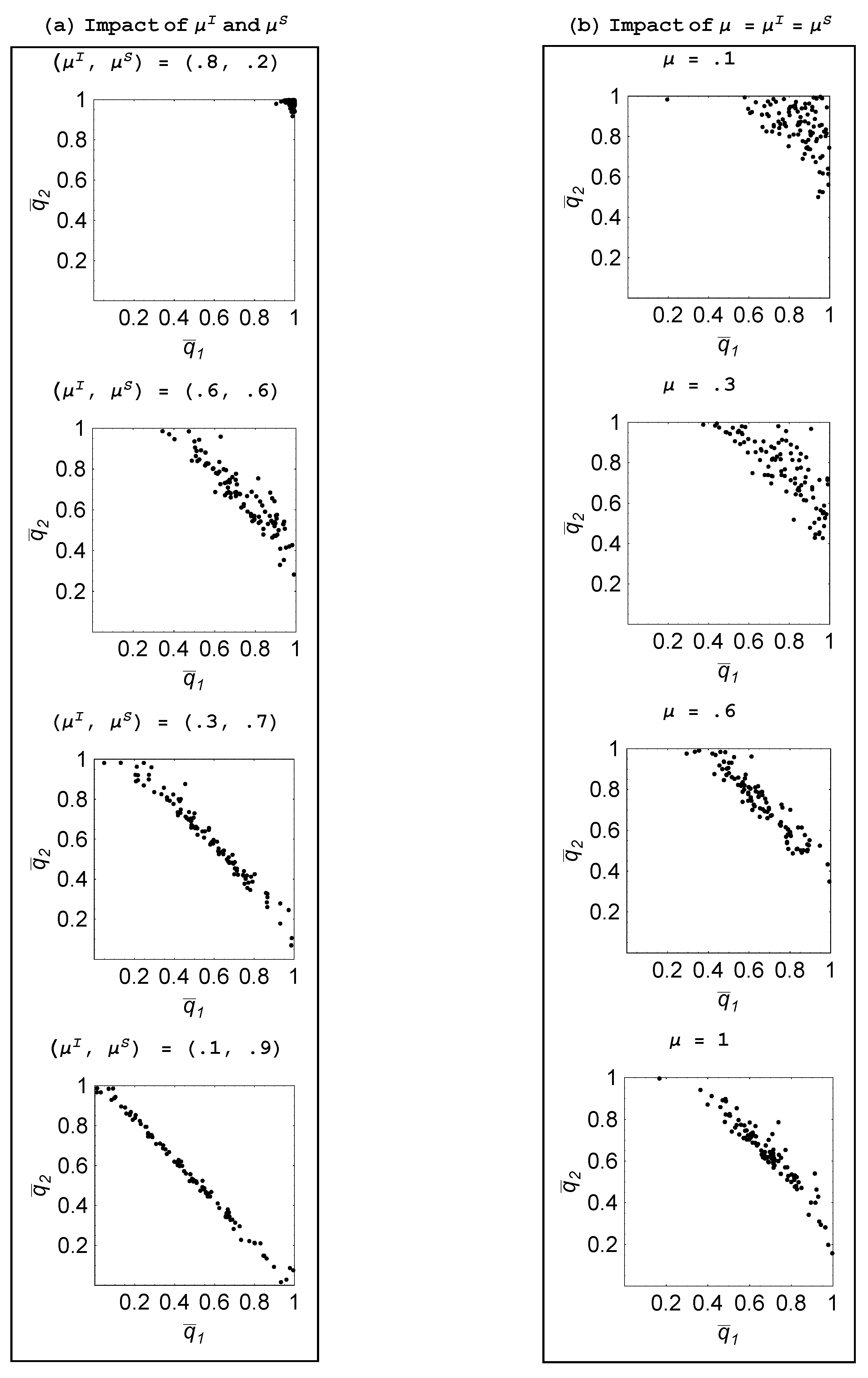
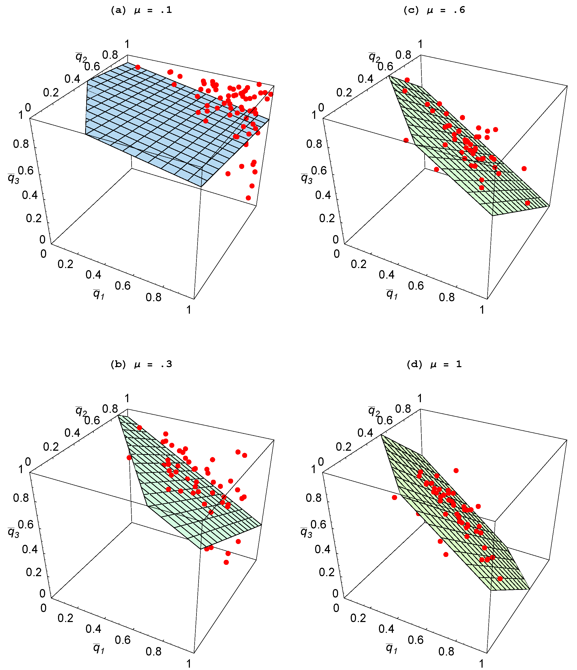
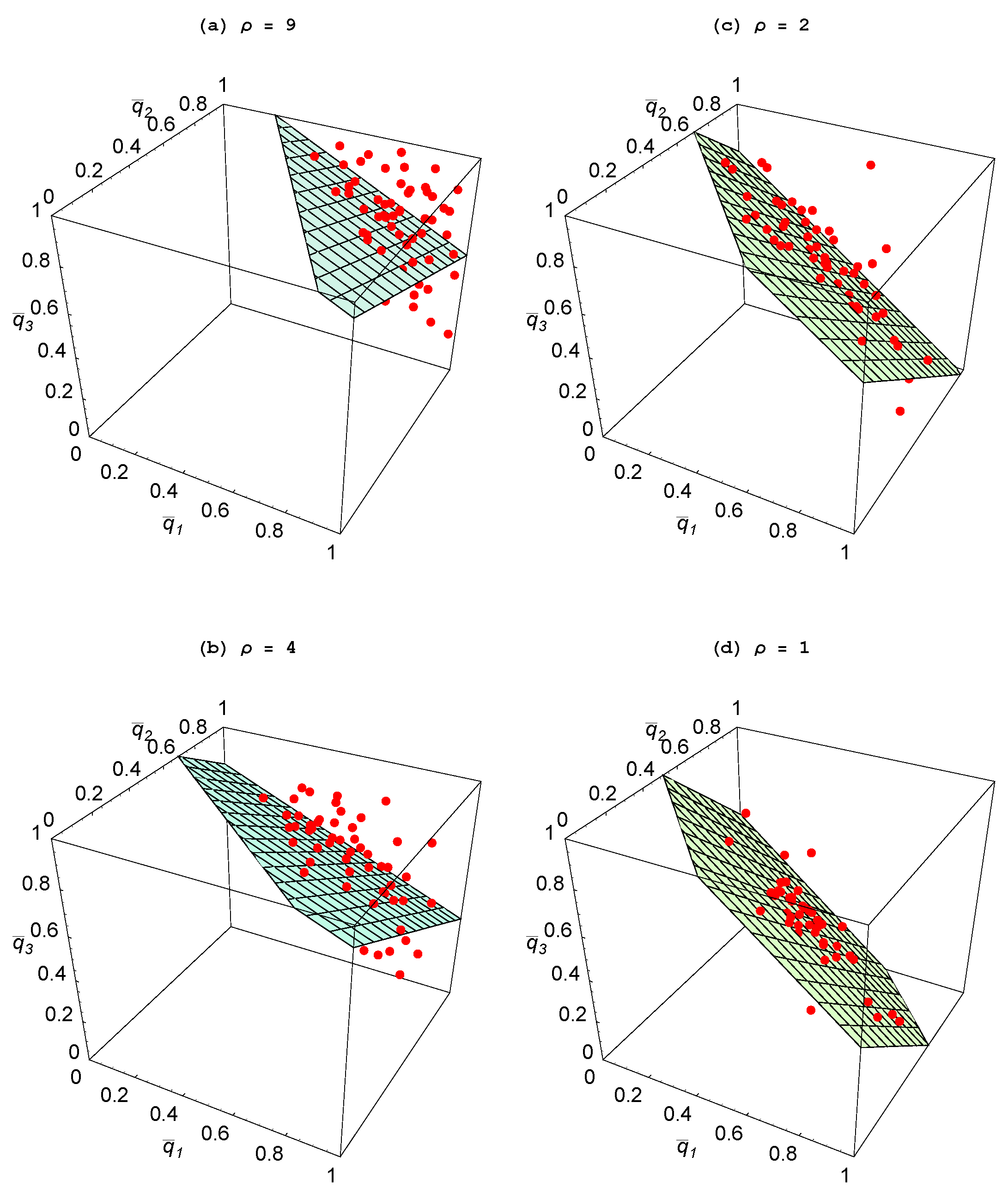
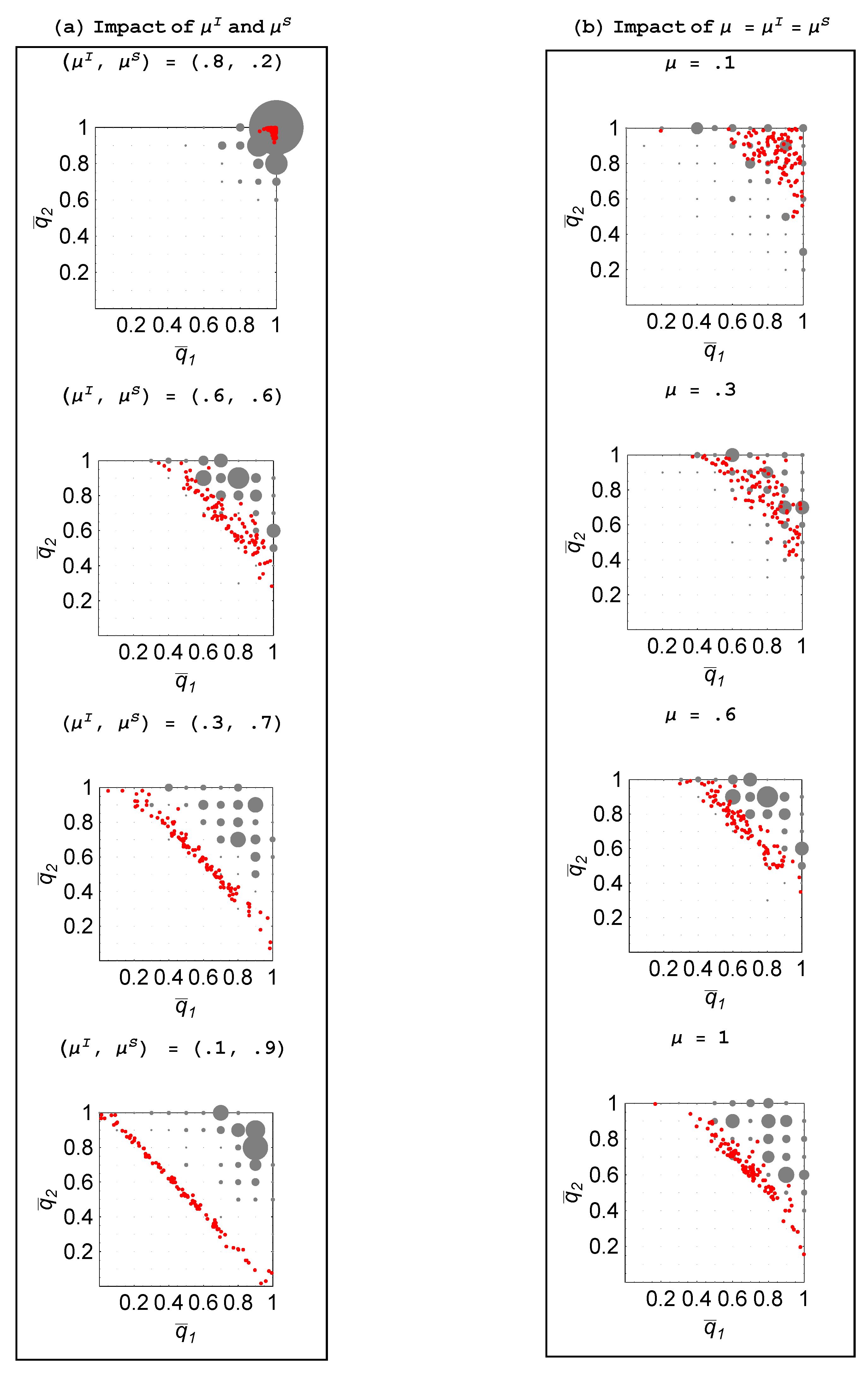
To establish the robustness of this phenomenon of specialization and explore its determinants, the same exercise was performed for ( μ I , μ S ) { ( 0 . 1 , 0 . 9 ) , ( 0 . 3 , 0 . 7 ) , ( 0 . 6 , 0 . 6 ) , ( 0 . 8 , 0 . 2 ) } and for both two-agent and three-agent populations. Figure 4(a) plots the 100 realizations of the steady-state probability pairs for L = 2 . Starting with ( μ I , μ S ) = ( 0 . 8 , 0 . 2 ) — so that agents are quite effective at individual learning but inadequate at social learning—we find that there is little social learning as both agents focus on trying to come up with ideas on their own. As μ S is raised and μ I is reduced—so that agents become relatively more proficient at social learning—we naturally find that agents spend less time in the individual learning mode. This is reflected in the steady-state probabilities shifting in towards the origin. What is more interesting is that the structure of specialization begins to emerge, whereby one agent focuses on individual learning and the other focuses on social learning. This is also shown for a three-agent population in Figure 5 where we have plotted q ¯ 1 , q ¯ 2 , q ¯ 3 . To better visualize the relationship between these values, a two-dimensional plane has been fitted to these points using ordinary least squares. Analogous to that in Figure 4(a), as the relative productivity of agents in social learning rises, the fitted plane shifts in and moves toward the unit simplex. Hence, once again, structure emerges in the form of specialization so that when one agent is heavily focusing on individual learning, the other agents are largely engaged in social learning.
When μ I is relatively low and μ S is relatively high, it is clear that it would not be best for all agents to largely engage in social learning as then there would be few new ideas arising and thus little to imitate. Though it could so happen that all agents choose to engage in some individual learning—such as with the replications that end up with q ¯ 1 , q ¯ 2 , q ¯ 3 0 . 33 , 0 . 33 , 0 . 33 —what also emerges in some replications is that one agent chooses to largely focus on individual learning. As then there are many new ideas streaming into the population, the other two agents focus on imitating and end up spreading the ideas of others. The result is a dramatic divergence in the choice of learning mechanisms, indicating a sharp division of cognitive labor.
Property 2 For populations with two or three agents, specialization is greater when agents are relatively more skilled in social learning than in individual learning.
Figure 4. Impact of learning skills ( σ = 0 . 8 , ρ = 1 ).
Admsci 03 00053 g004
Figure 5. Impact of learning skills ( σ = 0 . 8 , ρ = 1 ).
Admsci 03 00053 g005
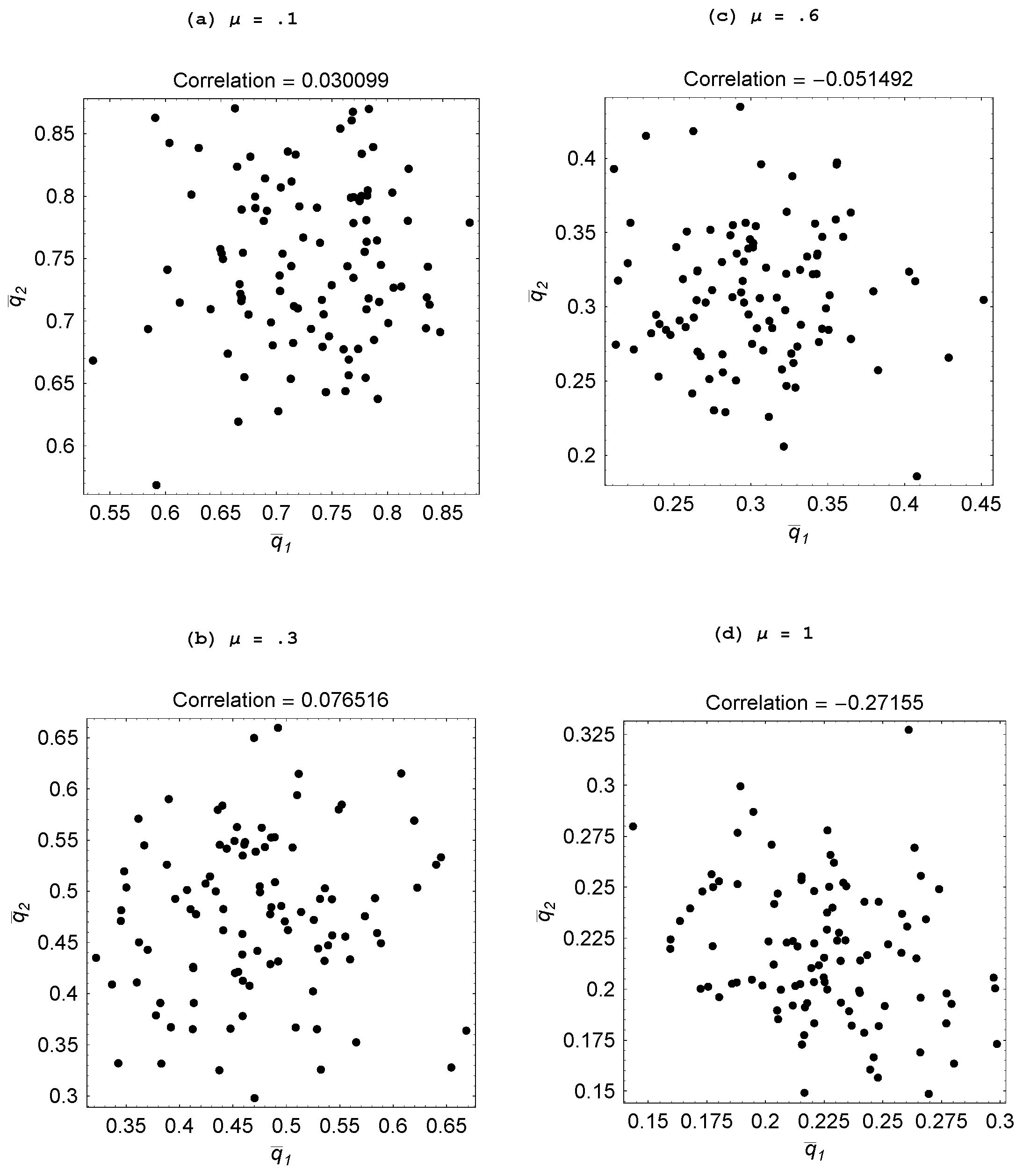
Figure 6. Impact of μ ( σ = 0 . 8 , ρ = 1 ).
Admsci 03 00053 g006
Figure 4(b) and Figure 6 explore what happens when agents are equally skilled at these two tasks, μ I = μ S μ , and we make them more skilled by raising μ . As μ is progressively raised from 0.1 to 1, agents engage in less individual learning and more specialization emerges. When agents are relatively unskilled, ideas are scarce and furthermore when social learning finally succeeds in finding an idea, it is apt to be “old” and thus was adopted for an environment distinct from the current one. In contrast, ideas discovered through individual learning will not suffer from being “old.” As a result, agents largely engage in individual learning when unskilled. As they become more skilled, social learning proves more productive—both because other agents are producing more ideas and social learning discovers them faster—so we observe agents engaging in less individual learning. But what also happens is there is more specialization as, if one agent is heavily engaged in individual learning, then the other agents free-ride by focusing on social learning.
Property 3 For populations with two or three agents, specialization is greater when agents are more skilled in both individual and social learning.
From Figure 4, Figure 5 and Figure 6, one can conclude that the key parameter is the productivity of agents with respect to social learning, μ S . When it is low - regardless of whether μ I is low or high—agents largely engage in individual learning and little structure emerges. When μ S is at least moderately high, specialization can emerge whether or not agents are relatively effective in individual learning. If agents are effective at communicating with each other then the environment is ripe for heterogeneous roles to arise in spite of the homogeneity of agents’ skills.
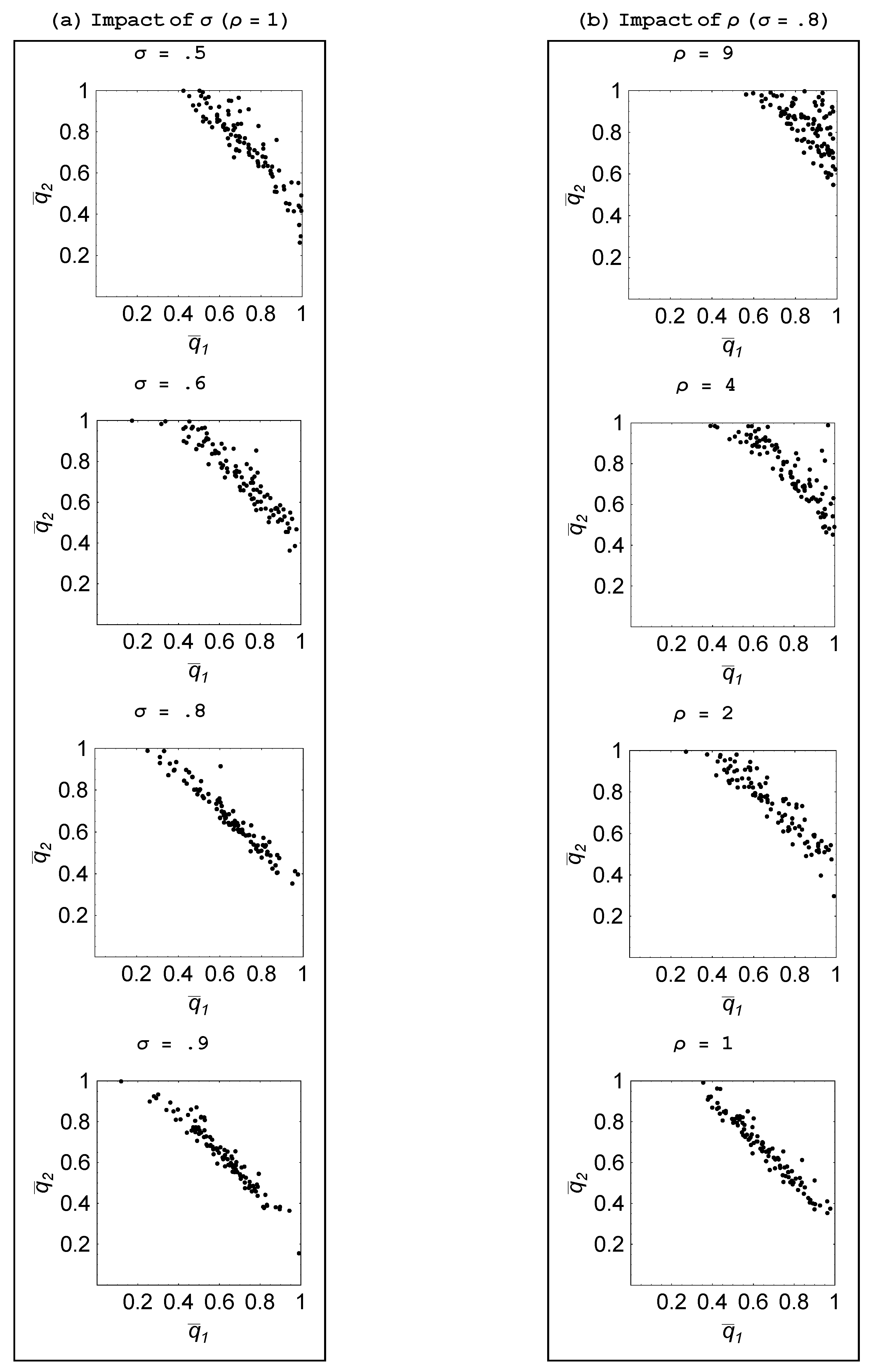
An interesting comparative static is to assess how the volatility of the environment affects the emergence of specialization. Recall that σ is the probability with which the goal vector shifts in a given period, while ρ represents the number of tasks in which change occurs. Figure 7 shows how making the environment more stable—as reflected in a rise in σ and a fall in ρ—impacts outcomes for a two-agent population, while analogous results are reported in Figure 8 and Figure 9 for when there are three agents. These results lead us to the following statement:
Property 4 For populations with two or three agents, specialization is greater when the environment is more stable.
A more volatile environment calls for a higher rate of adaptation by the agents. Recall that there is delay associated with the social learning process in that the process entails one agent discovering an idea that is useful for the current environment and then another agent learning that idea. By the time this social learning takes place, the environment could have changed which then makes this idea unattractive. Hence, social learning is relatively less productive when the environment is changing at a faster rate—as with a lower value for σ—or involves bigger changes—as with a higher value for ρ. It is then only when there is sufficient persistence in the environment, that social learning becomes effective enough that some agents choose to specialize in it and learn from an agent who focuses on individual learning.
To provide additional support for the above four properties, note that q ¯ i represents the probability with which agent i chooses individual learning along the steady-state. The likelihood of specialization being observed in a two-agent population is then represented by ω ¯ , where ω ¯ = q ¯ 1 ( 1 q ¯ 2 ) + q ¯ 2 ( 1 q ¯ 1 ) . This measures the likelihood that exactly one agent engages in individual learning, while the other engages in social learning along the steady-state. As there are 100 independent trials, we have 100 realizations of ω ¯ for each parameter configuration. Table 1 reports the mean and standard deviation of ω ¯ s obtained in these replications. As expected, the likelihood of specialization monotonically increases in μ S μ I , μ , and σ, while it decreases in ρ.
Figure 7. Impact of environmental volatility ( μ I = μ S = 1 ).
Admsci 03 00053 g007
Figure 8. Impact of σ ( μ I = μ S = 1 ; ρ = 1 ).
Admsci 03 00053 g008
Figure 9. Impact of ρ ( μ I = μ S = 1 ; σ = 0 . 8 ).
Admsci 03 00053 g009
Table 1. Mean and Standard Deviation of ω ¯ over 100 Replications.
Parameters ω ¯
μ I μ S σρMeanStd. Dev.
Impact of ( μ I , μ S )0.80.20.810.03301970.0204064
0.60.60.810.4656960.0630542
0.30.70.810.5685670.103349
0.10.90.810.6223610.137291
Impact of μ ( = μ I = μ S ) 0.10.10.810.2794220.107147
0.30.30.810.3958290.0891995
0.60.60.810.4709370.0568553
110.810.4926380.0794427
Impact of σ110.510.4412560.0749621
110.610.4625140.0723325
110.810.4966720.0605297
110.910.5176760.0722354
Impact of ρ110.810.4971520.0528074
110.810.4580650.0636729
110.810.3937310.0770097
110.810.2833330.0781933

4.2. Social Sub-Optimality of Endogenous Specialization

The previous results characterize agent behavior when they are acting independently and responding to their own individual performance. How does the resulting allocation between individual learning and social learning compare with what would maximize aggregate steady-state performance of the population? Due to computational constraints, this question we addressed only for the case of a two agent population. 100 trials were performed and, for each trial, we carried out the learning process with two agents for each of the 121 probability pairs, ( q 1 , q 2 ) , where q i { 0 , 0 . 1 , 0 . 2 , 0 . 3 , 0 . 4 , 0 . 5 , 0 . 6 , 0 . 7 , 0 . 8 , 0 . 9 , 1 } , i = 1 , 2 . [To perform an analogous exercise for when there are three agents would require doing this for 1,331 triples of ( q 1 , q 2 , q 3 ) .] The pair, ( q 1 , q 2 ) , was constrained to remain fixed for the entire horizon of 15 , 000 periods. For each ( q 1 , q 2 ) pair, the mean steady-state performance for the population, π ¯ , was computed as specified in Equation (14). Comparing among those π ¯ s, the socially optimal probability pair, ( q 1 * , q 2 * ) , was identified for a given trial: Since the population size is fixed at L, the aggregate steady-state performance of the population is simply L · π ¯ and the derivation of ( q 1 * , q 2 * ) can be based on the comparisons among π ¯ s. Given that there are 100 trials in total, we then have 100 realizations of the socially optimal probability pair.
Figure 10 and Figure 11 plot these social optima for different parameter configurations (in exactly the same format as the previous figures). The coordinates of the center of a grey disc represents the occurrence of that probability pair as the social optimum, while the frequency (among the 100 trials) with which it was a social optimum is represented by the size of the disc: The larger the disc, the greater is the frequency. The endogenous probability pairs from Figure 4 and Figure 7 have been superimposed to allow for an easier comparison. As before, Figure 10 considers the impacts of μ I / μ S and μ, while Figure 11 examines the impacts of σ and ρ.
Figure 10. ( q ¯ 1 , q ¯ 2 ) vs. ( q 1 * , q 2 * ) given σ = 0 . 8 and ρ = 1 .
Admsci 03 00053 g010
Figure 11. ( q ¯ 1 , q ¯ 2 ) vs. ( q 1 * , q 2 * ) given μ I = μ S = 1 .
Admsci 03 00053 g011
The central property we observe is that the social optimum, generally, entails more individual learning by both agents than that which emerges under autonomous choice rules. Left to engaging in reinforcement learning on their own, agents tend to imitate too much and innovate too little.
Property 5 For a two-agent population, agents engage in excessive social learning. The deviation from the socially optimal level of social learning tends to: (1) increase in μ S relative to μ I ; (2) increase in μ; (3) increase in σ; and (4) decrease in ρ.
Note that the deviation from the social optimum tends to be more severe in those cases where there exists a greater divergence in the steady-state probabilities. This implies that the circumstances more favorable to social learning and, hence, free-riding are also the ones which cause deviations from the social optimum to a greater extent.

5. Learning in Moderately-Sized Populations

The objective of this section is to determine to what extent the properties identified for small populations extend to larger populations. In particular, is it still the case that structure emerges in the form of specialization? For this purpose, the model was re-run for all L { 5 , 10 , 20 , 50 } . For each population size, a vector of steady-state individual learning probabilities, q ¯ 1 , q ¯ 2 , , q ¯ L , was then derived for each of 100 trials. For brevity, we will only report results for when there are 20 agents; the results for the other population sizes are similar.
The primary challenge was in effectively reporting the results for those runs. Obviously, we cannot use the visualization methods deployed in Section 4 as plotting the 100 realizations of q ¯ 1 , , q ¯ 20 would require a 20-dimensional figure! Our approach is instead as follows. First, partition the population into two equal-sized sets. As L = 20 , there are then 10 agents in group I and 10 agents in group II. For each set, calculate the average propensity for individual learning:
q ¯ I = 1 10 i = 1 10 q ¯ i , q ¯ I I = 1 10 i = 11 20 q ¯ i
Plotting the 100 realizations of q ¯ I , q ¯ I I , we can then assess to what extent there is a negative correlation between them. That is, when one group of agents engages in more individual learning does the other group of agents free-ride and engage in more social learning. Note that this is a generalization of the method used when L = 2 .
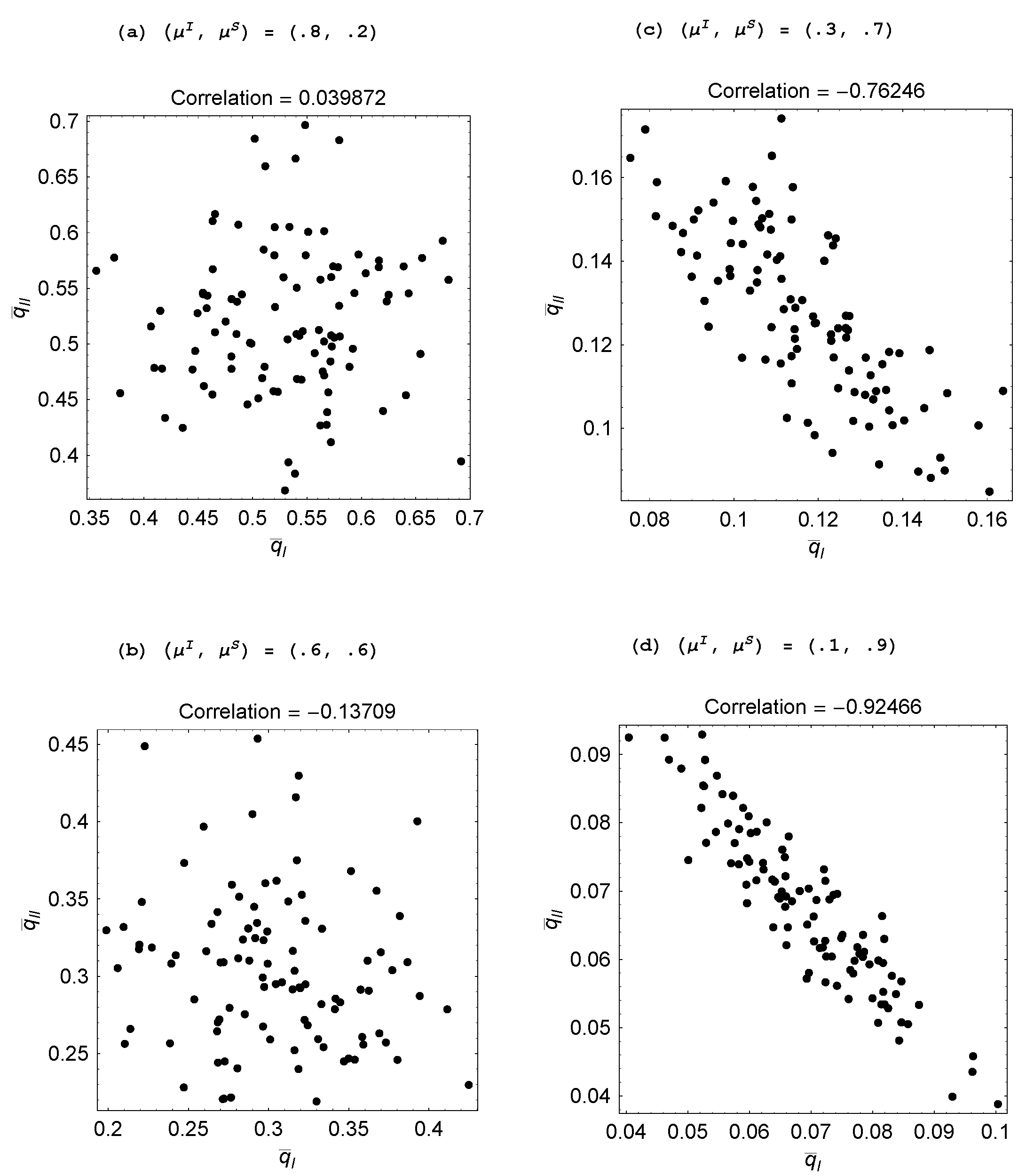
When μ I , μ S = 0 . 8 , 0 . 2 , Figure 12(a) shows that there is not much of relationship between the propensities for individual learning of the two groups. However, as μ S is raised and μ I is reduced, structure emerges. The correlation (which is reported at the top of each figure) becomes increasingly negative and visually q ¯ I and q ¯ I I line up as was found for two-agent populations. Note, however, that the size of the effect is distinctly smaller. For example, when μ I , μ S = 0 . 3 , 0 . 7 , if group I innovates with probability around 0.16 (which is the maximum value for q ¯ I over the 100 trials) then group II tends to do so with about half the probability at 0.08. In comparison, when there are only two agents, the extreme values entail one agent almost exclusively engaging in individual learning and the other agent almost exclusively engaging in social learning. It is important to keep in mind that our measure of specialization is apt to dilute its effect since it is comparing the average behavior of half the population with the average behavior of the other half. More importantly, these findings show that the emergence of specialization is quite general regardless of the population size.
Property 6 When agents are sufficiently more skilled in social learning than in individual learning, specialization emerges. The extent of specialization is increasing in μ S / μ I .
In Figure 14 and Figure 15, the specialization that emerges with μ I , μ S = 0 . 3 , 0 . 7 is shown to be robust to the stability of the environment as reflected in various values for σ and ρ. However, we do not find evidence of Property 4 in that our measure of specialization—the negative correlation between q ¯ I and q ¯ I I —is not greater when the environment is more stable. This is very likely due to the lack of sensitivity of our measure to what a few agents might be doing.
Figure 12. Impact of μ I and μ S ( σ = 0 . 8 , ρ = 1 ).
Admsci 03 00053 g012
Figure 13. Impact of μ ( σ = 0 . 8 , ρ = 1 ).
Admsci 03 00053 g013
Figure 14. Impact of σ ( μ I = 0.3; μ S = 0.7; ρ = 1).
Admsci 03 00053 g014
Figure 15. Impact of ρ ( μ I = 0.3; μ S = 0.7; σ = 0.8).
Admsci 03 00053 g015

6. Conclusions

In Chang and Harrington [4], we showed that an improvement in communication technology, which raises the social learning skills of the population, can induce excessive homogenization of the practices adopted by the agents. The consequent lack of diversity in the pool of ideas then reduces the potential for long-term progress. In this paper, we have identified yet another problem that could result from improved social learning skills of the population—the endogenous bifurcation of the population into individual learners and social learners and the consequent free-riding which proves socially sub-optimal. A natural next question, which is left for future research, is what kinds of social and organizational norms and structures might serve to guide the learning behavior of agents and serve to counteract these unproductive tendencies.

Conflict of Interest

The authors declare no conflict of interest.

References

  1. Hawn, C. If he’s so smart ... Steve Jobs, Apple, and the limits of innovation. Fast Company, 78. 1 January 2004, p. 68. Available online: http://www.fastcompany.com/48286/if-hes-so-smartsteve-jobs-apple-and-limits-innovation (accessed on 9 July 2013).
  2. Playing monopoly. News Hour with Jim Lehrer Transcript. 14 April 1998. Available online: http://www.pbs.org/newshour/bb/law/jan-june98/microsoft-4-14.html (accessed on 9 July 2013).
  3. Kitcher, P. The Advancement of Science: Science Without Legend, Objectivity Without Illusions; Oxford University Press: Oxford, England, 1993. [Google Scholar]
  4. Chang, M.H.; Harrington, J.E. Discovery and diffusion of knowledge in an endogenous social network. Am. J. Sociol. 2005, 110, 937–976. [Google Scholar] [CrossRef]
  5. Chang, M.H.; Harrington, J.E. Innovators, imitators, and the evoloving architecture of problem-solving networks. Organ. Sci. 2007, 18, 648–666. [Google Scholar] [CrossRef]
  6. Chang, M.H. Emergent social learning networks in organizations with heterogeneous agents. Adv. Complex Syst. 2011, 14, 169–199. [Google Scholar] [CrossRef]
  7. Kuhn, T.S. The Structure of Scientific Revolutions, 3rd ed.; The University of Chicago Press: Chicago, USA, 1996. [Google Scholar]
  8. Camerer, C.; Ho, T.H. Experience-weighted attraction learning in normal form games. Econometrica 1999, 67, 827–874. [Google Scholar] [CrossRef]