Article

Existence, Uniqueness and Stability of Market Equilibrium in Oligopoly Markets

by
Yulia Dzhabarova
1,
Stanimir Kabaivanov
2,*,
Margarita Ruseva
3 and
Boyan Zlatanov
4,*
1
Department of Marketing and International Economic Relations, Faculty of Economics and Social Sciences, University of Plovdiv Paisii Hilendarski, 4000 Plovdiv, Bulgaria
2
Department of Finance and Accounting, Faculty of Economics and Social Sciences, University of Plovdiv Paisii Hilendarski, 4000 Plovdiv, Bulgaria
3
Department of Management and Quantitative Economicsx, Faculty of Economics and Social Sciences, University of Plovdiv Paisii Hilendarski, 4000 Plovdiv, Bulgaria
4
Department of Mathematical Analysis, Faculty of Mathematics and Informatics, University of Plovdiv Paisii Hilendarski, 4000 Plovdiv, Bulgaria
*
Authors to whom correspondence should be addressed.
Adm. Sci. 2020, 10(3), 70; https://doi.org/10.3390/admsci10030070
Submission received: 7 August 2020 / Revised: 24 August 2020 / Accepted: 1 September 2020 / Published: 6 September 2020

Abstract

:
In this paper we build a pragmatic model on competition in oligopoly markets. To achieve this goal, we use an approach based on studying the response functions of each market participant, thus making it possible to address both Cournot and Bertrand industrial structures with a unified formal method. In contrast to the restrictive theoretical constructs of duopoly equilibrium, our study is able to account for real-world limitations like minimal sustainable production levels and exclusive access to certain resources. We prove and demonstrate that by using carefully constructed response functions it is possible to build and calibrate a model that reflects different competitive strategies used in extremely concentrated markets. The response functions approach makes it also possible to take into consideration different barriers to entry. By fitting to the response functions rather than the profit maximization of the payoff functions problem we alter the classical optimization problem to a problem of coupled fixed points, which has the benefit that considering corner optimum, corner equilibria and convexity condition of the payoff function can be skipped.
JEL Classification:
C02; D43; C62

1. Introduction

Markets dominated by a small number of players are getting more common than ever. This process has been fueled by industry consolidation, rise in international expansion and natural desire to benefit from economies in scale, all resulting in a number of mergers and acquisitions that leave few companies dominating a particular market. Cournot in 1838, in Cournot (1897), was the first to build a complete model of a market where few players control the price and supply quantity of the goods being traded. The original model is able to correctly estimate equilibrium conditions provided that market participants comply with the following requirements:
(i)
There are two players each with sufficient market power to affect the price of the goods being sold;
(ii)
There is no product differentiation;
(iii)
Decisions on production output are taken simultaneously;
(iv)
There is no cooperation between market participants and each one reacts in a rational way, seeking to maximize its profit.
If the two companies are not necessarily rational, a different solution can be found as for example in (Rubinstein 2019; Ueda 2019).
Cournot’s approach is known nowadays as a static oligopoly model, which means that each company, participating in the oligopoly market considers the production of others to remain fixed at least for a given period of time, i.e., player i assumes that in time t the other participants produce the quantities that they have produced in time t 1 . In the dynamic case, each company attempts to guess what change of production the other players will make in time t Cellini and Lambertini (2004).
Cournot’s duopoly model can be divided into two kinds—symmetric and asymmetric Sinha (2016). In the latter case, we consider an efficient company and a less-efficient one, producing homogeneous goods. Both are asymmetric in terms of their pre-innovation production costs. While both companies may have a fixed marginal cost of production, the efficient one has a lower cost c 1 , and the less-efficient one has a higher cost c 2 —where c 1 < c 2 . Companies still compete in quantities, as in Cournot’s duopoly. In the symmetric case both firms are equally efficient. It is important to note under which case a particular market falls, because asymmetric oligopoly may also end up dealing with products that are similar but of different quality. This is a question that falls beyond the scope of our study and we shall assume that there is no significant difference in the quality characteristics of the products produced and sold by each market participant.
Considering the demand, there are two distinct cases that have to be analyzed:
(i)
Demand is known and does not change. In this case the Cournot’s duopoly solution applies as it is.
(ii)
Demand may change over time. In the case, it is possible to reach a situation in which there is uncertainty about market equilibrium—as in Zapata et al. (2019).
We analyze a special case of Cournot’s duopoly in which the participating companies face different market demand in each of the scenarios.
A generalization of Cournot’s model is the Stackelberg duopoly Anderson and Engers (1992), where one firm is a leader and the other is a follower. This model is applicable when firms choose their output sequentially and not simultaneously. Cournot’s model and equilibrium are in fact the direct predecessor of Nash’s equilibrium point. Bertrand has introduced another kind of a duopoly model, where firms compete on prices rather than on outputs.
Contemporary markets can be subject to different regulations and barriers. Thus there are constraints applicable that influence the stability of market equilibrium and time required to reach it. We can summarize these constraints as:
(a)
The number of market participants;
Starting with the duopoly case in Cournot’s seminal work Cournot (1897) it is important to take into account the scalability of suggested solutions, due to the fact that there are various market structures in contemporary economics with high concentration and limited number of players.
(b)
The interdependence, availability, and access to information;
Companies operating in an environment with high concentration ratios (as measured by share of the largest participants compared to the total market volume) cannot take decisions in a completely isolated way. They need to take into account the effects their decisions have on the other participants, as well as their imminent reaction.
(c)
The price and non-price competition terms;
In order to account for the actual behavior of companies operating under oligopoly markets, it is necessary to take into consideration the non-price competition. In some cases, product differentiation may not exist (for example in the case of raw materials) but there may be loyalty schemes or aggressive advertisement campaigns that affect the equilibrium in an indirect way.
(d)
Consistency of behavior and time dependence of market conditions;
Solutions that consider time-dependency of company behavior and market changes Barbagallo and Cojocaru (2009) and Chan et al. (2018) are better able to describe contemporary oligopoly markets.
(e)
Market entry and exit barriers;
Entry and exit barriers can directly influence the number of companies operating on the oligopoly market. They also play an important role in shaping the decisions of each participant as barriers can be considered as additional limiting/boundary conditions.
(f)
Goals and profit maximization behavior;
We assume that profit maximization is the sole purpose of all market participants in the oligopoly markets. It is possible that there are periods of time, or even specific markets in which this is not the case (for example as described in Klemm 2004) and the resulting equilibrium is different. In the long term, economic agents would need to go back to profit maximization as they may be otherwise subject to acquisition or change in management.
(g)
Linear and non-linear changes in market conditions and firm behavior.
Taking into consideration these critical factors is very important in order to create a formal description of oligopoly markets that is adequate to the reality we live in.
Restraints could emerge as milestones at every production stage, at a different scale, size and intensity. Moreover, each of the restraints could influence each other, in a different direction and with different strength, and in parallel they could be influenced by the introduced production system and the existing market environment. The market is a vital substance, and the environment in which it functions and “breathes” would challenge the play of both actors, and could perform various scenarios of their action. Hence, these influences could affect the preliminary set up goals and price-polices of each of the observed players.
An extensive study on the oligopoly markets can be found in Bischi et al. (2010); Matsumoto and Szidarovszky (2018); Okuguchi (1976); Okuguchi and Szidarovszky (1990). Some recent results on Oligopoly markets are Alavifard et al. (2020); Geraskin (2020); Siegert and Ulbricht (2020); Strandholm (2020); Xiao and Wang (2020) and especially in duopoly markets Baik and Lee (2020); Liu and Sun (2020); Wang et al. (2020). All these items cannot be exhausted, even the published research on the subject in 2020. It is seen from the cited items that different techniques can be applied. We will present a different approach for the investigation of equilibrium in duopoly markets, based on the response functions, cyclic maps and coupled fixed (or best proximity) points.

2. Modeling Real-World Oligopoly Markets

Let us consider two companies that offer identical goods or services. These could range from health-care in a specific region to simple grocery delivery in a neighborhood. While the assumption for having homogeneous goods is quite restrictive, it helps to start with a simple model and then extend it by adding non-price competition and brand loyalty, to name a few extra factors. In support of the approach we have used, it should be noted that oligopoly markets with heterogeneous goods can be analyzed with the same instruments as the ones we employ. The only requirement is to define and estimate parameters of the response function of each market participant. In the case of identical goods it is much easier to do this. For complex products that include a variety of factors, such as positioning through non-price attributes, response functions may be harder to define and are often composite ones.
To investigate the existence and uniqueness of market equilibrium we employ game theory terminology. This is supported by the notion that company profits depend on its own output, as well as on the production of the other market participants. Under duopoly markets the result fits naturally into game theory basic cases of strategic interaction. Thus the static Cournot’s oligopoly is a fully rational game, based on the following assumptions:
(i)
Each company, in taking its optimal production decision rationally, must know before hand all its rival’s production and both firms should take their decisions simultaneously;
(ii)
Each firm has a perfect knowledge of the market demand function.
The dynamic model is a game in which case restrictive assumption (i) is replaced by some kind of expectation on the rivals’ outputs. While the simplest way is to use naive expectation that production or each market participant will remain at its most recent level, it is also possible to impose more realistic views as in McManus and Quandt (1961); Teocharis (1960). As a starting point, let us consider a situation in which there are two players ”A“ and ”B“ producing at moment n + 1 goods F ( x n , y n ) and f ( x n , y n ) , provided that at moment n they have produced x n and y n respectively. Such general notation does not yet imply anything regarding market participants. Depending on the functions F ( x n , y n ) and f ( x n , y n ) the model can be static or dynamic, as well as symmetric or asymmetric.
However in order to have market equilibrium, the pair ( x , y ) should satisfy the equations x = F ( x , y ) and y = f ( x , y ) .
Thus we will search for sufficient conditions, depending only on the response functions, that will ensure the existence and uniqueness of the equilibrium pair. Compared to the classical approaches in oligopoly markets, this way has several important advantages:
  • It is possible to account for protective capacity present in contemporary production environments, which allows to have minimal (or even zero) marginal costs within some output ranges;
  • It is possible to assess whether the marker can reach equilibrium, regardless of the initial position;
  • And finally it is possible to assess the time necessary to reach equilibrium and whether this situation can remain stable.

3. The Basic Model

Let us first start with a duopoly model Friedman (2007) and Smith (1987)—two companies competing for the same consumers and striving to meet the demand with overall production of Z = x + y . The market price is defined as P ( Z ) = P ( x + y ) , which is the inverse of the demand function. Market players have cost functions c 1 ( x ) and c 2 ( y ) , respectively. Assuming that both firms are acting rationally, the profit functions are Π 1 ( x , y ) = x P ( x + y ) c 1 ( x ) and Π 2 ( x , y ) = y P ( x + y ) c 2 ( y ) of the first and the second firm, respectively. The goal of each company is to maximize its profit, i.e., max { Π 1 ( x , y ) : x , assuming that y is fixed } and max { Π 2 ( x , y ) : y , assuming that x is fixed } . Provided that functions P and c i , i = 1 , 2 are differentiable, we get the equations
Π 1 ( x , y ) x = P ( x + y ) + x P ( x + y ) c 1 ( x ) = 0 Π 2 ( x , y ) y = P ( x + y ) + y P ( x + y ) c 2 ( y ) = 0 .
The solution of (1) presents the equilibrium pair of production in the duopoly market Friedman (2007); Smith (1987).
Often Equations (1) have solutions in the form of x = b 1 ( y ) and y = b 2 ( x ) , which are called response functions (Friedman 2007).
It may turn out difficult or impossible to solve (1) thus it is often advised to search for an approximate solution. Another drawback, when searching for an approximate solution is that it may not be stable. Fortunately we can find an implicit formula for the response function in (1) i.e.,
x = c 1 ( x ) P ( x + y ) P ( x + y ) = F ( x , y ) and y = c 2 ( y ) P ( x + y ) P ( x + y ) = f ( x , y ) .
It is still possible that we may end up with response functions, that do not lead to maximization of the profit Π . As it is often assumed, each participant response depends on its own production level and that of the pother payers. For example, if at a moment n the output quantities are ( x n , y n ) , and the first player changes its productions to x n + 1 = F ( x n , y n ) , then the second one will also change its output to y n + 1 = f ( x n , y n ) . We will define the iterated sequence { ( x n , y n ) } n = 1 in the Appendix A in Definition A5. We have an equilibrium if there are two productions x and y, such that x = F ( x , y ) and y = f ( x , y ) . The functions Π i are called payoff functions. To ensure that the solutions of (1) will present a maximization of the payoff functions, a sufficient condition is that Π i are concave functions Bischi et al. (2010); Matsumoto and Szidarovszky (2018); Okuguchi and Szidarovszky (1990), by using of response function we alter the maximization problem into a coupled fixed point one thus all assumptions of concavity and differentiability can be skipped. The problem of solving the equations x = F ( x , y ) and y = f ( x , y ) is the problem of finding coupled fixed points for an ordered pair of maps ( F , f ) Guo and Lakshmikantham (1987). Yet an important limitation may be that players cannot change the output too fast and thus the player may not perform to maximize their profits.
Focusing on response functions, allows to put together Cournot and Bertand models. Indeed let the first company have reaction be F ( X , Y ) and the second one f ( X , Y ) , where X = ( x , p ) and Y = ( y , q ) . Here x and y denote the output quantity and ( p , q ) are the prices set by players. In this case companies can compete in terms of both price and quantity.

4. Existence and Uniqueness in Duopoly Models

In the case of two major players taking all or most of the market, we need to consider special cases depending on intersection of production set. The situation in which production sets of both companies have an empty intersection may seem extreme, but it is not impossible. For example if one of the companies is working at a very large scale it may simply be impractical to sustain a low level of output. On the other hand, if the company is just too small to undertake large projects it may also happen that expanding its production beyond a certain limit is not feasible. Therefore, it is possible that long term contracts or technical issues prohibit a certain type of action and impose special limitations. The mathematical justifications of the results are presented in Appendix A.

4.1. Players’ Production Sets Have a Nonempty Intersection

Assumption 1.
Let there be a duopoly market, satisfying the following assumptions:
(1) 
The two firms are producing homogeneous goods that are perfect substitutes.
(2) 
The first firm can produce qualities from the set A x and the second firm can produce qualities from the set A y , where A x and A y be closed, nonempty subsets of a complete metric space ( X , ρ ) .
(3) 
Let there exist a closed subset D A x × A y and maps F : D A x and f : D A y , such that ( F ( x , y ) , f ( x , y ) ) D for every ( x , y ) D , be the response functions for firm one and two respectively.
(4) 
Let there exist α , β , γ , δ > 0 , max { α + γ , β + δ } < 1 , such that the inequality
ρ ( F ( x , y ) , F ( u , v ) ) + ρ ( f ( z , w ) , f ( t , s ) ) α ρ ( x , u ) + β ρ ( y , v ) + γ ρ ( z , t ) + δ ρ ( w , s )
holds for all ( x , y ) , ( u , v ) , ( z , w ) , ( t , s ) A x × A y .
Then
(I)
There exists a unique pair ( ξ , η ) in D, such that ξ = F ( ξ , η ) and η = f ( ξ , η ) , i.e., a market equilibrium pair. Moreover the iteration sequences { x n } n = 0 and { y n } n = 0 , defined in Definition A5 converge to ξ and η respectively.
(II)
A priori error estimates hold
max ρ ( x n , ξ ) , ρ ( y n , η ) k n 1 k ( ρ ( x 1 , x 0 ) + ρ ( y 1 , y 0 ) ) ;
(III)
A posteriori error estimates hold
max ρ ( x n , ξ ) , ρ ( y n , η ) k 1 k ( ρ ( x n 1 , x n ) + ρ ( y n 1 , y n ) ) ;
(IV)
The rate of convergence for the sequences of successive iterations is given by
ρ ( x n , ξ ) + ρ ( y n , η ) k ρ ( x n 1 , ξ ) + ( y n 1 , η ) ,
where k = max { α + γ , β + δ } .
If in addition f ( x . y ) = F ( y , x ) then the coupled fixed point ( x , y ) satisfies x = y .
The proof is a direct consequence of Theorem A1.
Remark 1.
Let the two players have one and the same response function. That is if player one has a production x and player two has a production y then the first player reaction will be F ( x , y ) and the second player reaction will be f ( x , y ) = F ( y , x ) . It follows that the equilibrium pair ( x , y ) will satisfy x = y , i.e., both firms will have equal production. This means that if both firms have one and the same technology, one and the same knowledge on the market that will affect to one and the same response functions, then the equilibrium will be reached at the level of equal productions.

4.2. Equilibrium, When Players’ Production Sets Have a Nonempty Intersection

Let us consider a duopoly market. Let the two firms produce qualities from the set A x and the second firm can produce qualities from the set A y , where A x and A y are nonempty subsets of a complete metric space ( X , ρ ) . Any of the firms can produce a bundle of products x = ( x 1 , x 2 , x n ) X . Assumption 1 ensures the existence and uniqueness of the production bundles ( x 1 , x 2 , x n ) , ( y 1 , y 2 , y n ) X of n-goods, that present the equilibrium in a duopoly economy.

4.2.1. A Linear Case, When Each Player Is Producing a Single Product, Goods Being Perfect Substitutes

Let us consider a market with two competing firms, each firm producing just one product, and both goods are perfect substitutes. Let the two firms produce quantities x A x and y A y , respectively, where A x , A y [ 0 , + ) and ( X , ρ ) be the complete metric space ( R , | · | ) . Let us consider the response functions of player one F ( x , y ) = a s p x q y and player two f ( x , y ) = a r μ y ν x , where
(1)
a , s , r , p , q , μ , ν > 0 , s < a , r < a , max { p + μ , q + ν } < 1
(2)
A x = 0 , a s p 0 , a r μ and A y = 0 , a s q 0 , a r ν
(3)
D can be defined in three ways:
(3a)
D = 0 , a μ a q s μ q r μ p ν q × 0 , a p a ν + s ν p r μ p ν q , provided that
a s a μ a q s μ q r μ p ν q and a r a p a ν + s ν p r μ p ν q
(3b)
D = 0 , a s × 0 , a r , provided that μ r + ν s a μ a ν + a r > 0 and p s + q r a p a q + a s > 0
(3c)
D = 0 x a s p 0 y a r μ x ν .
It is easy to check that F : D A x × A y A x , f : D A x × A y A y and ( F ( D ) , f ( D ) ) D .
Indeed let us consider case (3a). From the assumptions that a , s , r , p , q , μ , ν > 0 we get
F ( x , y ) F ( 0 , 0 ) = a s a μ a q + s μ q r μ p ν q ,
F ( x , y ) F a μ a q + s μ q r μ p ν q , a p a ν + s ν p r μ p ν q = 0 ,
and
f ( x , y ) f ( 0 , 0 ) = a r a p a ν + s ν p r μ p ν q ,
f ( x , y ) f a μ a q + s μ q r μ p ν q , a p a ν + s ν p r μ p ν q = 0 .
Therefore F : D A x , f : D A y and ( F ( D ) , f ( D ) ) D .
It can be proven in a similar fashion that ( F ( D ) , f ( D ) ) D and for the cases (3b) and (3c).
From the inequalities
F ( x , y ) F ( u , v ) = p ( x u ) + q ( y v ) p | x u | + q | y v |
and
f ( z , w ) f ( t , s ) = μ ( z t ) + ν ( w s ) μ | z t | + ν | w s |
it follows that
F ( x , y ) F ( u , v ) + f ( z , w ) f ( t , s ) p | x u | + q | y v | + μ | z t | + ν | w s |
and thus the ordered pair ( F , f ) satisfies Assumption 1 with constants α = p , β = q , γ = μ , δ = ν , because max { p + μ , q + ν } < 0 . Consequently there exists an equilibrium pair ( x , y ) and for any initial start in the economy the iterated sequences ( x n , y n ) converge to the market equilibrium ( x , y ) . The equilibrium pair is
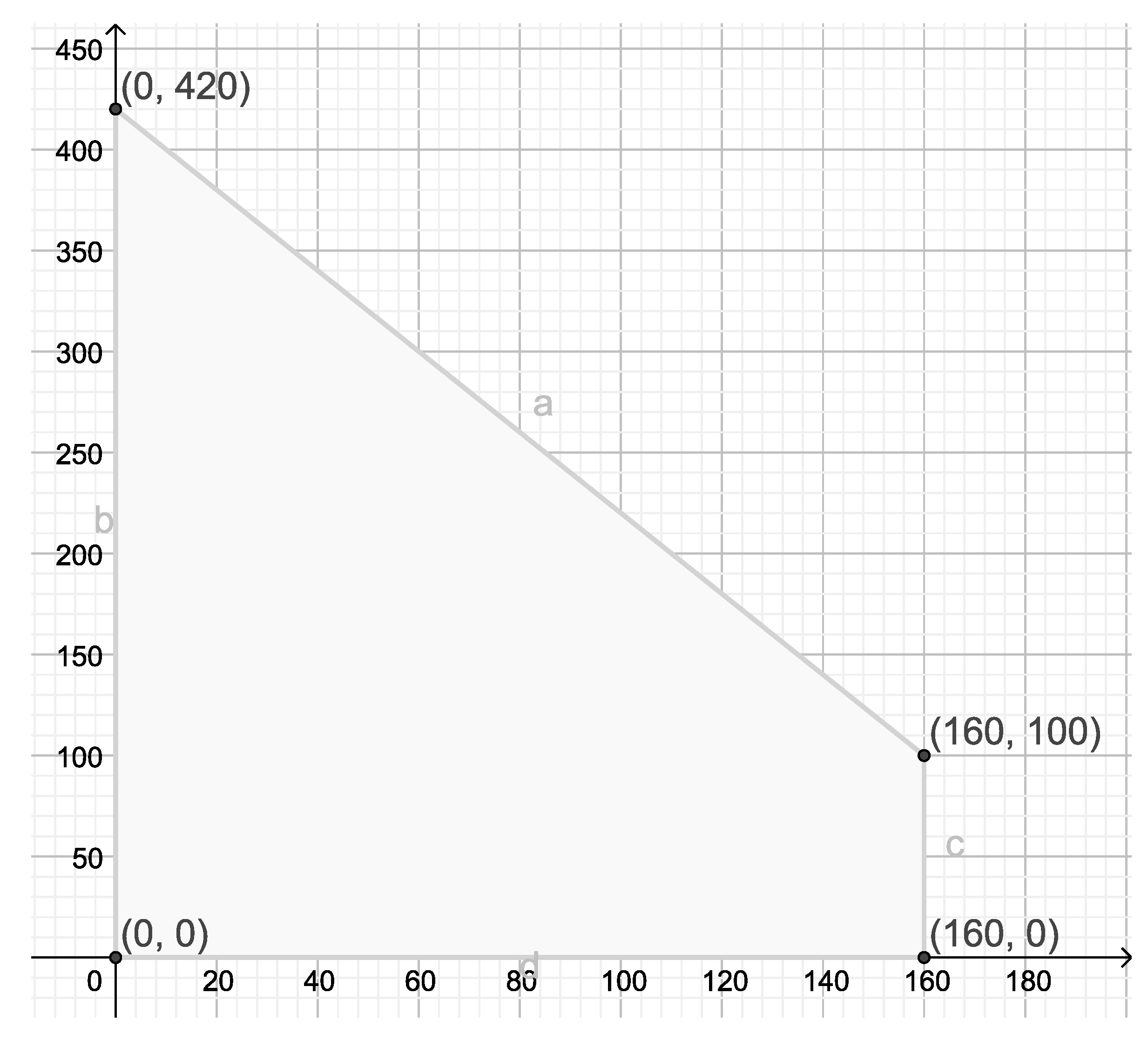
x = a μ a q s μ + q r + a s μ p ν q + μ + p + 1 , y = a p a ν + s ν p r a + r μ p ν q + μ + p + 1 .
Let us consider a particular case: a = 100 , s = 20 , r = 30 , p = 1 2 , q = 1 8 , μ = 1 3 , ν = 1 6 .
Values selected for this case are arbitrarily chosen with only general conditions in mind. However, in an actual situation the values of p, q, μ and ν reflect the actual management and marketing policy of the market participants.
In this case F ( x , y ) = 80 x 2 y 8 , f ( x , y ) = 70 x 3 y 6 , A x = [ 0 , 210 ] , A y = [ 0 , 320 ] . The subset D can be considered either D = [ 0 , 110 ] × [ 0 , 200 ] (3a) or D = { 0 x 160 , 0 y 420 2 x } (3c) (see Figure 1).
We get in this case that the equilibrium pair of the production of the two firms is ( 49.51 , 45.85 ) and the total production will be x + y = 95.36 . Values of the iterated sequence are presented in Table 1 and numbers of iterations needed for the a priori and a posteriori error estimate are shown in Table 2 and Table 3, respectively.
To get the data to fill the above tables and the tables in the forthcoming examples we use Maple 2016 software.
Let us consider a classic example, where the price function is linear and so are the cost functions of both players. Assuming the feasible market price is defined by P ( x , y ) = 120 x y , it is expected that additional output x from the first company as well as extra production y of the second one will cause a decrease in prices. Therefore under equilibrium conditions x + y will be the total production of the two firms and it will also be reflected in prices. Let the two firms have cost functions equal to 30 x and 20 y , respectively. The profit of the first one is
Π 1 ( x , y ) = x P ( x , y ) 30 x = x ( 120 x y ) 30 x = 90 x x 2 x y
and the profit of the second one is
Π 2 ( x , y ) = y P ( x , y ) 20 y = y ( 120 x y ) 20 y = 100 y y 2 x y .
Following the Cournot model after solving (1) we get the response functions F : D A x and f : D A y of the two firms F ( y ) = 90 y 2 and f ( x ) = 100 x 2 , where A y = [ 0 , 90 ] , A x = [ 0 , 100 ] and D = A x × A y . Consequently it is a special case of the general example with a = 60 , s = 15 , r = 10 , p = 0 , q = 1 2 , μ = 1 2 , ν = 0 .
It is possible to find the constants in this case with the help of some Computer Algebra System (CAS), such as Maple, MathLab, MathCad or Mathematica. We will illustrate it by using Maple 2016. Writing the command
s o l v e 90 y 2 90 v 2 p | y v | , 0 y 90 , 0 v 90 , a ;
the software returns that p 1 2 . The same result can be obtained and for the inequality | f ( x ) f ( u ) | μ | x u | . Unfortunately when trying to solve the forthcoming more complicated examples Maple was not of good use, therefore we have preferred to use some of the classical inequalities and to make the calculations by hand.
Thus there exists an equilibrium pair ( x , y ) and for any initial start in the economy where iterated sequences ( x n , y n ) converge to the market equilibrium ( x , y ) . We estimate in this case that the equilibrium pair of the production is ( 80 / 3 , 110 / 3 ) and the total output will be a = 190 / 3 .
Let us assume that the two firms have started with output x 0 = 40 and y 0 = 60 . In the following table (see Table 4) we present how, depending on the response functions F and f the output of each company will change.
Let us assume that the two firms have started from productions x 0 = 100 and y 0 = 20 . In the next table (see Table 5) we present how using the response functions F and f the productions of the two firms will change.
Numbers of iterations needed for the a priori and a posteriori error estimate are shown in Table 6 and Table 7 are presented in the case ( x 0 = 100 , y 0 = 20 ) , respectively.

4.2.2. A Nonlinear Case, When Each Player Is Producing a Single Product, While Goods Sold Are Perfect Substitutes

Let us consider a market with two competing firms, producing perfect substitute products with quantities x A x and y A y , respectively, where A x , A y [ 0 , + ) and ( X , ρ ) is the complete metric space ( R , | · | ) . Let us assume that each firm produces at least one item, i.e., x , y 1 . Let us consider the response functions of player one F ( x , y ) = 90 x y 8 y 2 2 and player two f ( x , y ) = 100 x 4 y x 3 , where
  • A x = [ 1 , 44 ] and A y = [ 1 , 33 ]
  • D can be defined as D = A x × A y
It is easy to check that F : D = A x × A y A x , f : D = A x × A y A y and ( F ( D ) , f ( D ) ) D .
Indeed, we get
F ( x , y ) F ( 1 , 1 ) = 44 , F ( x , y ) F 44 , 33 = 13.31
and
f ( x , y ) f ( 1 , 1 ) = 32.33 < 33 , f ( x , y ) f 44 , 33 = 5.46
and therefore F : D A x , f : D A y and ( F ( D ) , f ( D ) ) D .
There exists ξ between the points y and v so that there holds y v = 1 2 ξ | y v | . From the assumption that y , v 1 we get that y v 1 2 | y v | . Using this last inequality we obtain
F ( x , y ) F ( u , v ) 1 2 x u + 1 16 y v + 1 8 y v = 1 2 x u + 3 16 y v
and
f ( z , w ) f ( t , s ) 1 12 z t + 1 3 w s + 1 6 w s = 1 12 z t + 1 2 w s .
Therefore
F ( x , y ) F ( u , v ) + f ( z , w ) f ( t , s ) 1 2 x u + 3 16 y v + 1 12 z t + 1 2 w s
and thus the ordered pair ( F , f ) satisfies Assumption 1 with constants α = 1 / 2 , β = 3 / 16 , γ = 1 / 12 and δ = 1 / 2 , max { 1 / 2 + 1 / 12 , 3 / 16 + 1 / 2 } = max { 7 / 12 , 11 / 16 } = 7 / 12 . Consequently there exists an equilibrium pair ( x , y ) and for any initial start in the economy the iterated sequences ( x n , y n ) converge to the market equilibrium ( x , y ) . We get in this case that the equilibrium pair of the production of the two firms is ( 28.3 , 21.9 ) (see Table 8) and the total production will be a = 50.2 . Number of the needed iterations is presented in Table 9 and Table 10.
If we try to solve the system of equations x = F ( x , y ) and y = f ( x , y ) from the previous section, where for example F ( x , y ) = 80 x 2 y 8 and f ( x , y ) = 70 x 3 y 6 , with the help of Maple then we will get the exact result. Unfortunately when the response functions are not linear the software can give us just some approximation. No information is available about the uniqueness and the stability of the solution. The same observations have been made in Zlatanov (2021), the exact solution is possible to find with the help of the theory of coupled best proximity points, but the approximation solution, regardless of the precision, is never the exact one.
Let us consider again a case with two players, producing two products, but let them know the market demand function and behave rational, i.e., they are trying to maximize their profits, assuming that the rival player will do the same.
Let there be no limit on the market, but let us assume that the total consumption is 100 % . That is, the market will consume a constant 1, which is 100 % , and the production of both firms will be a percentage of the consumption x and y, respectively, i.e., x , y [ 0 , 1 ] . Let the market price be defined by P ( x , y ) = 1 x + y 2 x 2 + y 2 24 , where x is the production of one of the firms, y is the production of the other one, assuming that number 1 presents 100 % . Let the two firms have cost functions equal to C x ( x ) = x / 2 + x 2 / 16 and y / 6 + y 2 / 12 , respectively. The profit of the first firm is
Π 1 ( x , y ) = x P ( x , y ) C x ( x ) = 7 x 8 9 x 2 16 x y 2 x 3 24 x y 2 24
and the profit of the second firm is
Π 2 ( x , y ) = y P ( x , y ) C y = 5 y 6 13 y 2 24 x y 2 y 3 24 x 2 y 24 .
Following Cournot model after solving (1) we get the response functions F and f of the two players
F ( x , y ) = 7 8 x 8 y 2 x 2 8 y 2 24 and f ( x , y ) = 5 6 x 2 y 12 y 2 8 x 2 24 ,
which satisfy F : [ 0 , 1 ] × [ 0 , 1 ] [ 0 , 1 ] and f : [ 0 , 1 ] × [ 0 , 1 ] [ 0 , 1 ] , i.e., D = [ 0 , 1 ] × [ 0 , 1 ] . Using the inequality | x 2 y 2 | = 2 ξ | x y | 2 | x y | , for any x , y [ 0 , 1 ] and some ξ between x and y we obtain
F ( x , y ) F ( u , v ) 3 8 | x u | + 7 12 | y v |
and
f ( z , w ) f ( s , t ) 7 12 | z t | + 7 24 w s .
Therefore
F ( x , y ) F ( u , v ) + f ( z , w ) f ( s , t ) 3 8 x u + 7 12 | y v | + 7 12 | z s | + 7 24 w t
and thus the ordered pair ( F , f ) satisfies Assumption 1 with constants α = 3 / 8 , β = 7 / 12 , γ = 7 / 12 and δ = 7 / 24 . There holds max { α + γ , β + δ } < 0.958 . Thus there exists an equilibrium pair ( x , y ) and for any initial start in the economy the iterated sequences ( x n , y n ) converge to the market equilibrium ( x , y ) . We get in this case that the equilibrium pair of the production of the two firms is ( 0.537 , 0.451 ) , i.e., the first firm will have a share of 53.7 % and the second one a share of 45.1 % of the sold goods (see Table 11 if the starting point is ( 50 % , 50 % ) , Table 12 if the starting point is ( 10 % , 90 % ) and Table 13 if the starting point is ( 100 % , 0 % ) ). The total production will be 0.989 , i.e., 98.9 % of the total demand of the market.

4.2.3. Each Player Is Producing Two Product Types, Goods from Each Type Being Perfect Substitutes

Let us consider a market with two competing firms, and each firm is producing two product types. For simplicity we assume that goods from each type produced by major players are perfect substitutes. While it is possible that two types have nothing it common, it still means that within each type customers can freely replace a product from the first company with one manufactured by the second one. Let us assume that each firm produces at least one item from each product, i.e., x = ( x 1 , x 2 ) , y = ( y 1 , y 2 ) , x 1 , x 2 , y 1 , y 2 1 . Let us denote the production of the two players by x = ( x 1 , x 2 ) and y = ( y 1 , y 2 ) , respectively.
Let the market of the two goods be endowed with the p norm, p [ 1 , ) , i.e.,
ρ ( ( x 1 , x 2 ) , ( y 1 , y 2 ) ) = ( x 1 , x 2 ) ( y 1 , y 2 ) p = | x 1 y 1 | p + | x 2 y 2 | p 1 / p .
Let us consider the response functions F ( x , y ) = ( F 1 ( x , y ) , F 2 ( x , y ) ) and f ( x , y ) = ( f 1 ( x , y ) , f 2 ( x , y ) ) defined by
F ( x , y ) = 90 x 1 + x 2 2 y 1 + y 2 3 3 , 90 x 1 + x 2 2 y 1 + y 2 3 3 ; f ( x , y ) = 100 x 1 + x 2 4 y 1 + y 2 3 4 100 x 1 + x 2 4 y 1 + y 2 3 4 .
where
  • A x = [ 0 , 30 ] × [ 0 , 30 ] and A y = [ 0 , 25 ] × [ 0 , 25 ]
  • D = [ 0 , 30 ] × [ 0 , 30 ] × [ 0 , 25 ] × [ 0 , 25 ]
It is easy to see that ( F ( x , y ) , f ( x , y ) ) D , whenever ( x , y ) = ( ( x 1 , x 2 ) , ( y 1 , y 2 ) ) D .
Using the inequality a + b 2 ( a p + b p ) 1 / p 2 1 / p , which holds for any a , b 0 we get the chain of inequalities
F ( x , y ) F ( u , v ) p = F 1 ( x , y ) , F 2 ( x , y ) F 1 ( u , v ) , F 2 ( u , v ) p = ( u 1 + u 2 ) ( x 1 + x 2 ) 2 + v 1 + v 2 ( y 1 + y 2 ) 3 3 , ( u 1 + u 2 ) ( x 1 + x 2 ) 2 + v 1 + v 2 ( y 1 + y 2 ) 3 3 p 2 3 | u 1 x 1 | + | u 2 x 2 | 2 + | v 1 y 1 | + | v 2 y 2 | 3 = 2 3 | u 1 x 1 | + | u 2 + x 2 | 2 + 4 9 | v 1 y 1 | + | v 2 + y 2 | 2 2 p 1 p 3 | x 1 u 1 | p + | x 2 y 2 | p 1 / p + 2 p 1 p + 1 9 | y 1 v 1 | p + | y 2 v 2 | p 1 / p = 2 p 1 p 3 ( x 1 , x 2 ) ( u 1 , u 2 ) p + 2 p 1 p + 1 9 ( y 1 , v 2 ) ( y 1 , v 2 ) p = 2 p 1 p 3 x u p + 2 p 1 p + 1 9 y v p
and
f ( x , y ) f ( u , v ) p = f 1 ( x , y ) , f 2 ( x , y ) f 1 ( u , v ) , f 2 ( u , v ) p = ( u 1 + u 2 ) ( x 1 + x 2 ) 4 + v 1 + v 2 ( y 1 + y 2 ) 3 3 , ( u 1 + u 2 ) ( x 1 + x 2 ) 4 + v 1 + v 2 ( y 1 + y 2 ) 3 3 p 2 3 | u 1 x 1 | + | u 2 x 2 | 4 + | v 1 y 1 | + | v 2 y 2 | 3 = 2 6 | u 1 x 1 | | u 2 + x 2 | 2 + 4 9 | v 1 y 1 | + | v 2 + y 2 | 2 2 p 1 p 6 | x 1 u 1 | p + | x 2 y 2 | p 1 / p + 2 p 1 p + 1 9 | y 1 v 1 | p + | y 2 v 2 | p 1 / p = 2 p 1 p 6 ( x 1 , x 2 ) ( u 1 , u 2 ) p + 2 p 1 p + 1 9 ( y 1 , v 2 ) ( y 1 , v 2 ) p = 2 p 1 p 6 x u p + 2 p 1 p + 1 9 y v p .
Therefore
F ( x , y ) F ( u , v ) + f ( z , w ) f ( t , s ) 2 p 1 p x u 3 + z t 6 + 2 2 p 1 p y v 9 + w s 9 .
From the inequalities 2 p 1 p 3 + 2 p 1 p 6 < 2 3 + 1 3 = 1 and 2 2 p 1 p 9 + 2 2 p 1 p 9 2 4 9 < 1 it follows that the ordered pair ( F , f ) satisfies Assumption 1 with constants α = 2 p 1 p 3 , β = 2 p 1 p + 1 9 , γ = 2 p 1 p 6 and δ = 2 p 1 p + 1 9 . Thus there exists an equilibrium pair ( x , y ) and for any initial start in the economy the iterated sequences ( x n , y n ) converge to the market equilibrium ( x , y ) . We get in this case that the equilibrium pair of the production of the two firms is x = ( 19.27 , 19.27 ) , y = ( 19.36 , 19.36 ) (see Table 14 and Table 15) and the total production will be a = ( 38.63 , 38.63 ) . Numbers of iterations, that a needed to ensure the a priori (see Table 16) and the a posteriori (see Table 17) are calculated.

4.3. The Players Are Producing a Single Product and Compete on Both Quantities and Prices

There is a large number of goods where companies can compete on both quality and prices. In this case the equilibrium would depend on a balanced decision on what market share to target at a reasonable price. Let us assume that there are only two major players that produce homogeneous products. The first company can produce qualities from the set A x [ 0 , ) at a price p P x [ 0 , ) and the second one can produce qualities from the set A y [ 0 , ) at a price p P x [ 0 , ) , where A x , A y , P x , P y are nonempty subsets. Let A x × P x , A y × P y be subsets of a complete metric space ( R 2 , ρ ) .
Assumption 2.
Let there be a duopoly market, satisfying the following assumptions:
(1) 
The two firms are producing homogeneous, perfect substitute products.
(2) 
The first firm can produce qualities from the set A x at a price p P x and the second firm can produce qualities from the set A y at a price p P x , where A x × P x , A y × P y are nonempty, closed subsets of a complete metric space ( R 2 , ρ ) .
(3) 
Let there exist a closed subset D A x × P x × A y × P y A x , such that F : D A x × P x , f : D A y × P y and ( F ( x , p , y , q ) , f ( x , p , y , q ) ) D for every ( x , p , y , q ) D be the response functions for firm one and two respectively.
(4) 
Let there exist α , β , γ , δ > 0 , max { α + γ , β + δ } < 1 , such that the inequality
ρ ( F ( X , Y ) , F ( U , V ) ) + ρ ( f ( Z , W ) , f ( T , S ) ) α ρ ( X , U ) + β ρ ( Y , V ) + γ ρ ( Z , T ) + δ ρ ( W , S ) ,
where we use thenotations X = ( x , p 1 ) , Y = ( y , q 1 ) , U = ( u , p 2 ) , V = ( v , q 2 ) , Z = ( z , p 3 ) , W = ( w , q 3 ) , T = ( t , p 4 ) , S = ( s , q 4 ) , holds for all ( x , p 1 , y , q 1 ) , ( u , p 2 , v , q 2 ) , ( z , p 3 , w , q 3 ) , ( t , p 4 , s , q 4 ) D .
Then
(I)
There exists a unique pair ( ξ , p , η , q ) in A x × P x × A y × P y , which is a common coupled fixed point for the maps F and f, i.e., a market equilibrium pair. Moreover the iteration sequences { x n } n = 0 , { p n } n = 0 , { y n } n = 0 and { q n } n = 0 , defined in Definition A5 converge to ξ , p, η , and q respectively.
(II)
A priori error estimates hold
S 1 = max ρ ( ( x n , p n ) , ( ξ , p ) ) , ρ ( ( y n , q n ) , ( η , q ) ) k n 1 k ( ρ ( ( x 1 , p 1 ) , ( x 0 , p 0 ) ) + ρ ( ( y 1 , q 1 ) , ( y 0 , q 0 ) ) ) ;
(III)
A posteriori error estimates hold
S 2 = max ρ ( ( x n , p n ) , ( ξ , p ) ) , ρ ( ( y n , q n ) , ( η , q ) ) k 1 k ( ρ ( ( x n 1 , p n 1 ) , ( x n , p n ) ) + ρ ( ( y n 1 , p n 1 ) , ( y n , q n ) ) ) ;
(IV)
The rate of convergence for the sequences of successive iterations is given by
S 3 = ρ ( ( x n , p n ) , ( ξ , p ) ) + ρ ( ( y n , q n ) , ( η , q ) ) k ρ ( ( x n 1 , p n 1 , ( ξ , p ) ) + ρ ( ( y n 1 , p n 1 ) , ( η , q ) ) ,
where k = max { α + γ , β + δ } .
If in addition f ( X , Y ) = F ( Y , X ) then the coupled fixed point ( X , Y ) satisfies X = Y , i.e., x = y and p = q .
The proof is a direct consequence of Theorem A1.
Remark 2.
If we consider Bertrand’s model with the same assumption of equal response functions then not only the quantities will be equal but also and the prices.

Example of a Duopoly Model, Where Players Compete on Quantities and Prices Simultaneously

Let us consider a market with two competing firms, producing the same product, and selling it at a price p and q respectively, i.e., X = ( x , p ) , Y = ( y , q ) . Let us consider the response functions F ( X , Y ) = ( F 1 ( X , Y ) , F 2 ( X , Y ) ) and f ( X , Y ) = ( f 1 ( X , Y ) , f 2 ( X , Y ) ) defined by
F ( X , Y ) = 90 x 2 y 3 3 , 4 p 2 q 3 3 ; f ( X , Y ) = 100 x 4 y 3 4 5 p 4 q 3 4 .
Let X = ( x , p ) and Y = ( y , q ) be subsets of ( R 2 , · 2 ) (the two dimensional Euclidean space). Let
  • A x = [ 0 , 100 ] × [ 0 , 5 ] and A y = [ 0 , 100 ] × [ 0 , 4 ]
  • D = [ 0 , 100 ] × [ 0 , 5 ] × [ 0 , 100 ] × [ 0 , 4 ]
It is easy to see that F : D [ 0 , 100 ] × [ 0 , 5 ] , f : D [ 0 , 100 ] × [ 0 , 4 ] and ( F ( x , p , y , q ) , f ( x , p , y , q ) ) D for every ( x , p , y , q ) D .
Using the inequality a + b 2 ( a 2 + b 2 ) 1 / 2 2 1 / 2 , which holds for any a , b 0 we get the chain of inequalities we obtain
S 4 = F ( x , p 1 , y , q 1 ) F ( u , p 2 , v , q 2 ) 2 = 90 x 2 y 3 3 , 4 p 1 2 q 1 3 3 90 u 2 v 3 3 , 4 p 2 2 q 2 3 3 2 = u x 2 + v y 3 3 , p 1 p 2 2 + q 1 q 2 3 3 2 1 3 | u x | + | v y | 2 2 + | p 1 p 2 | + | q 1 q 2 | 2 2 1 3 | u x | + | v y | 2 + | p 1 p 2 | + | q 1 q 2 | 2 = 1 3 | u x | + | p 1 p 2 | 2 + | v y | + | q 1 q 2 | 2 1 3 2 | u x | 2 + | p 1 p 2 | 2 + 1 3 2 | v y | + | q 1 q 2 | = 1 3 2 ρ ( U , X ) + 1 3 2 ρ ( V , Y )
and
S 5 = f ( x , p 1 , y , q 1 ) f ( u , p 2 , v , q 2 ) 2 = 100 x 4 y 3 4 , 5 p 1 4 q 1 3 4 100 u 4 v 3 4 , 5 p 2 4 q 2 3 4 2 = u x 4 + v y 3 4 , p 1 p 2 4 + q 1 q 2 3 4 2 1 4 | u x | + | v y | 3 2 + | p 1 p 2 | + | q 1 q 2 | 3 2 1 4 | u x | + | v y | 3 + | p 1 p 2 | + | q 1 q 2 | 3 < 1 4 | u x | + | p 1 p 2 | 2 + | v y | + | q 1 q 2 | 2 1 4 2 | u x | 2 + | p 1 p 2 | 2 + 1 4 2 | v y | + | q 1 q 2 | = 1 4 2 ρ ( U , X ) + 1 4 2 ρ ( V , Y ) .
Therefore
F ( X , Y ) F ( U , V ) + f ( Z , W ) f ( T , S ) X U 3 2 + Y V 3 2 + Z T 4 2 + W S 4 2 .
From the inequalities 1 3 2 + 1 4 2 < 1 it follows that the ordered pair ( F , f ) satisfies Assumption 2 with constants α = 1 3 2 , β = 1 3 2 , γ = 1 4 2 and δ = 1 4 2 . Thus there exists an equilibrium pair ( x , y ) and for any initial start in the economy the iterated sequences ( x n , y n ) converge to the market equilibrium ( x , y ) . We get in this case that the equilibrium pair of the production of the two firms is x = ( 23.64 , 1.03 ) , y = ( 21.71 , 1.09 ) .

4.4. Players’ Production Sets Have an Empty Intersection

Assumption 3.
Let there be a duopoly market, satisfying the following assumptions:
1. 
The two firms are producing homogeneous perfect substitute products.
2. 
The first firm can produce qualities from the set A x and the second firm can produce qualities from the set A y , where A x and A y are nonempty, closed and convex subsets of a uniformly convex Banach space ( X , · )
3. 
Let there exist a closed and convex subset D A x × A y and maps F : D A x and f : D A y , such that ( F ( x , y ) , f ( x , y ) ) D for every ( x , y ) D , are the response functions for firm one and two respectively
4. 
Let there exist α , β > 0 , α + β < 1 , such that
F ( x , y ) f ( u , v ) α x v + β y u + ( 1 ( α + β ) ) d
for all ( x , y ) , ( u , v ) A x × A y , where d = dist ( A x , A y ) = inf { x y : x A x , y A y } .
Then there exists a unique pair ( ξ , η ) in A x × A y , which is a coupled best point for the pair of maps ( F , f ) , i.e., a market equilibrium pair. Moreover the iteration sequences { x n } n = 0 and { y n } n = 0 , defined in Definition A5 converge to ξ and η respectively.
If in addition ( X , · ) has a modulus of convexity of power type with constants C > 0 and q > 1 , then
  • A priori error estimates hold
    ξ x m M 0 max { W 0 , 1 ( x , y ) , W 0 , 0 ( x , y ) } C d q · ( α + β ) m q 1 α + β q ;
    η y m N 0 max { W 0 , 1 ( y , x ) , W 0 , 0 ( y , x ) } C d q · ( α + β ) m q 1 α + β q ;
  • A posteriori error estimates hold
    ξ x n M n 1 max { W n 1 , n ( x , y ) , W n 1 , n 1 ( x , y ) } C d q c .
    η y 2 n N n 1 max { W n 1 , n ( y , x ) , W n 1 , n 1 ( y , x ) } C d q c ,
    where W n , m ( x , y ) = x n x m d , M n max { x n y n , x n y n + 1 } , N n max { x n y n , y n x n + 1 } and c = α + β q 1 α + β q .
The proof is a direct consequence of Theorem A2.

Players’ Production Sets Have an Empty Intersection, Each Player Is Producing Two Goods

Let us consider a market with two competing firms, each firm produces two products and any one of the items is completely replaceable with a similar product of the other firm. Let us assume that the first firm can produce much less quantities than the second one, i.e., if x 1 , x 2 are the quantities produced by the first firm and y 1 , y 2 are the quantities produced by the second one and, then x 1 , x 2 [ 0 , 1 ] and y 1 , y 2 [ 2 , 3 ] . Let A x = [ 0 , 1 ] × [ 0 , 1 ] A y = [ 2 , 3 ] × [ 2 , 3 ] be considered as subsets of ( R 2 , · ) , which is a uniformly convex Banach space with modulus of convexity δ · 2 ( ε ) ε 2 3 of power type Zlatanov (2016). Let us consider the response functions F ( x 1 , x 2 , y 1 , y 2 ) and f ( x 1 , x 2 , y 1 , y 2 ) defined by
F ( x , y ) = 3 x 1 8 + x 2 8 3 y 1 16 y 2 16 + 1 x 1 8 + 3 x 2 8 y 1 16 3 y 2 16 + 1 , f ( x , y ) = 3 x 1 16 x 2 16 + 3 y 1 4 + y 2 4 + 5 4 x 1 16 3 x 2 16 + y 1 4 + 3 y 2 4 + 5 4 .
It is easy to see that F : [ 0 , 1 ] × [ 0 , 1 ] × [ 2 , 3 ] × [ 2 , 3 ] [ 0 , 1 ] × [ 0 , 1 ] and f : [ 0 , 1 ] × [ 0 , 1 ] × [ 2 , 3 ] × [ 2 , 3 ] [ 2 , 3 ] × [ 2 , 3 ]
Indeed the inequalities 0 3 x 1 8 + x 2 8 3 y 1 16 y 2 16 + 1 1 are equivalent to
3 y 1 16 + y 2 16 3 x 1 8 + x 2 8 + 1 3 x 1 8 + x 2 8 3 y 1 16 + y 2 16
for ( x 1 , x 2 , y 1 , y 2 ) [ 0 , 1 ] × [ 0 , 1 ] × [ 2 , 3 ] × [ 2 , 3 ] .
The inequalities 2 3 u 1 16 u 2 16 + 3 v 1 4 + v 2 4 + 5 4 3 are equivalent to
3 u 1 16 + u 2 16 3 v 1 4 + v 2 4 3 v 1 4 + v 2 4 7 4 + 3 u 1 16 + u 2 16
for ( u 1 , u 2 , v 1 , v 2 ) [ 0 , 1 ] × [ 0 , 1 ] × [ 2 , 3 ] × [ 2 , 3 ] .
Using the inequality 3 a 4 + b 4 2 3 4 a 2 + 1 4 b 2 , i.e., 3 a 4 + b 4 3 a 2 + b 2 2 we obtain
S 6 = F ( x 1 , x 2 , y 1 , y 2 ) f ( u 1 , u 2 , v 1 , v 2 ) 2 = 3 x 1 8 + x 2 8 3 y 1 16 y 2 16 + 1 , x 1 8 + 3 x 2 8 y 1 16 3 y 2 16 + 1 3 u 1 16 u 2 16 + 3 v 1 4 + v 2 4 + 5 4 , u 1 16 3 u 2 16 + v 1 4 + 3 v 2 4 + 5 4 2 = 1 4 + 3 ( x 1 v 1 ) 8 + x 2 v 2 8 , 1 4 + 3 ( u 1 y 1 ) 16 + u 2 y 2 16 2 1 4 , 1 4 2 + 3 ( x 1 v 1 ) 8 + x 2 v 2 8 , 3 ( u 1 y 1 ) 16 + u 2 y 2 16 2 2 4 + 3 ( x 1 v 1 ) 8 + x 2 v 2 8 , 0 2 + 0 , 3 ( u 1 y 1 ) 16 + u 2 y 2 16 2 = 2 4 + 1 2 3 ( x 1 v 1 ) 4 + x 2 v 2 4 , 0 2 + 1 4 0 , 3 ( u 1 y 1 ) 4 + u 2 y 2 4 2 = 2 4 + 1 2 3 ( x 1 v 1 ) 4 + x 2 v 2 4 + 1 4 3 ( u 1 y 1 ) 4 + u 2 y 2 4 2 2 4 + 3 | x 1 v 1 | 2 + | x 2 v 2 | 2 4 + 3 | u 1 y 1 | 2 + | u 2 y 2 | 2 8 2 4 + 3 4 | x 1 v 1 | 2 + | x 2 v 2 | 2 + 3 8 | u 1 y 1 | 2 + | u 2 y 2 | 2 = 3 4 x v 2 + 3 8 y u 2 + 2 4 3 4 x v 2 + 3 8 y u 2 + 1 3 4 3 8 2 = 3 4 x v 2 + 3 8 y u 2 + 1 3 4 3 8 d ,
where d = dist ( [ 0 , 1 ] × [ 0 , 1 ] , [ 2 , 3 ] × [ 2 , 3 ] ) = 2 . Therefore the ordered pair ( F , f ) satisfies Assumption 3 with constants α = 3 4 , β = 3 8 . Thus there exists an equilibrium pair ( x , y ) = ( ( x 1 , x 2 ) , ( y 1 , y 2 ) ) and for any initial start in the economy, the iterated sequence ( x n , y n ) = ( ( x 1 n , x 2 n ) , ( y 1 n , y 2 n ) ) converges to the market equilibrium ( x , y ) . We get in this case that the equilibrium pair of the production of the two firms is x = ( 1 , 1 ) , y = ( 2 , 2 ) (see Table 18 and Table 19) and the total production will be a = ( 3 , 3 ) .

4.5. Equilibrium in the Case, When the Two Players Are Producing Just One Good and the Production Set Has an Empty Intersection

Let us point out that the properties of the modulus of convexity δ · are investigated if the Banach space is at least two dimensional. As far as R , endowed with its canonical norm is a subspace of R 2 2 we get that δ ( R , | · | ) ( ε ) δ ( R 2 2 , · 2 ) ( ε ) = ε 2 8 . It is easy to observe that in R there holds the equality δ ( R , | · | ) ( ε ) = ε 2 . Indeed B ( R , | · | ) = [ 1 , 1 ] . Then δ ( R , | · | ) ( ε ) = inf 1 x + y 2 : x , y [ 1 , 1 ] , | x y | ε . The infimum is attained, when x = 1 and y = 1 ε . Therefore δ ( R , | · | ) ( ε ) = 1 1 + ( 1 ε ) 2 = ε 2 Ilchev and Zlatanov (2016).
We will formulate Assumption 3 in the case when the underlying Banach space is ( R , | · | ) .
Assumption 4.
Let there is a duopoly market, satisfying the following assumptions:
1. 
The two firms are producing homogeneous perfect substitute products
2. 
The first firm can produce qualities from the set A x and the second firm can produce qualities from the set A y , where A x and A y are nonempty closed intervals of ( R , | · | )
3. 
Let there exist a close and convex subset D A x × A y and maps F : D A x and f : D A y , such that ( F ( x , y ) , f ( x , y ) ) D for every ( x , y ) D , be the response functions for firm one and two respectively
4. 
Let there exist α , β > 0 , α + β < 1 , such that
| F ( x , y ) f ( u , v ) | α | x v | + β | y u | + ( 1 ( α + β ) ) d
for all ( x , y ) , ( u , v ) A x × A y , where d = dist ( A x , A y ) = inf { | x y | : x A x , y A y } .
Then there exists a unique pair ( ξ , η ) in A x × A y , which is a coupled best point for the pair of maps ( F , f ) , i.e., a market equilibrium pair. Moreover the iteration sequences { x n } n = 0 and { y n } n = 0 , defined in Definition A5 converge to ξ and η respectively.
  • A priori error estimates hold
    ξ x m 2 max { | x 0 y 0 | , | x 0 y 1 | } max { W 0 , 1 ( x , y ) , W 0 , 0 ( x , y ) } d · ( α + β ) m 1 ( α + β ) ;
    η y m 2 max { | x 0 y 0 | , | x 1 y 0 | } max { W 0 , 1 ( y , x ) , W 0 , 0 ( y , x ) } d · ( α + β ) m 1 ( α + β ) ;
  • A posteriori error estimates hold
    ξ x n 2 max { | x n 1 y n 1 | , | x n 1 y n | } max { W n 1 , n ( x , y ) , W n 1 , n 1 ( x , y ) } d ( 1 ( α + β ) ) ( α + β ) ;
    η y n 2 max { | x n 1 y n 1 | , | x n y n 1 | } max { W n 1 , n ( y , x ) , W n 1 , n 1 ( y , x ) } d ( 1 ( α + β ) ) ( α + β ) ,
    where W n , m ( x , y ) = | x n x m | d .
The proof is a direct consequence of Theorem A2 and the remark that ( R , | · | ) is a uniformly convex Banach space with modulus of convexity δ | · | ( ε ) = ε 2 .

Example When the Two Players Are Producing Just One Good

Let us consider a market with two competing firms, producing two products, that are perfect substitutes. Let us assume that the first firm can produce much smaller quantities than the second one, i.e., x , y , so that x [ 0 , 1 ] and y [ 2 , 3 ] . Let us consider the response functions F ( x , y ) and f ( x , y ) defined by
F ( x , y ) = x 2 y 4 + 1 , f ( x , y ) = u 4 + v 2 + 5 4
It is easy to see that F : [ 0 , 1 ] × [ 2 , 3 ] [ 0 , 1 ] and f : [ 0 , 1 ] × [ 2 , 3 ] [ 2 , 3 ]
Indeed the inequalities 0 x 2 y 4 + 1 1 are equivalent to
y 4 x 2 + 1 x 2 y 4
for ( x , y ) [ 0 , 1 ] × [ 2 , 3 ] .
The inequalities 2 u 4 + v 2 + 5 4 3 are equivalent to
3 4 + u 4 v 2 v 2 7 4 + u 4
for ( u , v ) [ 0 , 1 ] × [ 2 , 3 ] .
Then we obtain
| F ( x , y ) f ( u , v ) | = u 4 + v 2 + 5 4 x 2 y 4 + 1 | v x | 2 + | y u | 4 + 5 4 1 = | v x | 2 + | y u | 4 + 1 4 = | v x | 2 + | y u | 4 + 1 1 2 + 1 4 d .
Therefore the ordered pair ( F , f ) satisfies Assumption 4 with constants α = 1 2 , β = 1 4 . Thus there exists an equilibrium pair ( x , y ) and for any initial start in the economy the iterated sequences ( x n , y n ) converge to the market equilibrium ( x , y ) . We get in this case that the equilibrium pair of the production of the two firms is x = 1 , y = 2 (see Table 20, Table 21 and Table 22) and the total production will be a = 3 .

5. Conclusions

Markets dominated by a small group of players are not uncommon even in a fast moving global economy. Therefore it is essential to analyze these cases, understand what leads to equilibrium and how different companies respond to changes in the economic environment. In this paper we have built a model on existence and uniqueness of market equilibrium in oligopoly markets that can be derived from response functions of major players. We assume that goods produced by different market players are perfect substitutes as this simplifies the mathematical description of the model. Due to the fact that response functions can also account for differences in product qualities, the model can also be applied to situations where price is not the only factor on which companies compete. With a carefully constructed response function it is possible to fully comprehend all five basic factors influencing competition—product features, number of sellers, information ability and barriers to entry.
Use of the suggested model can help understand better markets with limited number of players. By solving the inverse problem—estimate response functions based on historical prices and output series, it is also possible to understand how companies make decisions and react on regulations and changes in the environment. Compared to other approaches that also allow to estimate how market participants change their behavior, our suggestion is more flexible and can be extended to include different limitations.
Response functions also support the concept of having protective capacity and the ability to change output within certain limits, with minimal changes in total costs. While this matches the way contemporary businesses are run, it also provides for building more realistic views of the market. That is of particular importance for taking regulatory measures and estimating how changes in economic conditions may affect certain industries. It should be noted that our approach is important also for a wider audience when we consider that there are rare metals and raw materials markets with oligopolistic structure. Such special cases have influence reaching beyond the trade with a particular good.
Existence and uniqueness of equilibrium can be analyzed with both linear and non-linear response functions which proves to be a very flexible approach when studying different markets, which despite being dominated by a small number of companies may have quite different characteristics. Applications of the suggested model when production sets of market participants have empty intersection are particularly important when it is necessary to account for real world limitations like huge economies of scale or unique resources available to some players. One specific application and advantage of the suggested model is that calibration of response functions can be performed in a way that matches observed past behavior (output and prices) or major market players. This way it is possible to assess not only equilibrium stability but also the way that different companies react to changes in the environment.

Author Contributions

The listed authors (Y.D., S.K., M.R. and B.Z.) have made equal contributions to the presented research. All authors have read and agreed to the published version of the manuscript.

Funding

The research is partially supported by the NPD-Plovdiv University under grant No. FP19-FESS-014 “Contemporary tools and approaches for economic and business analysis” and by the Project KP-06 K2-29: “Integral model for forecasting and prevention” of socio–economic effects of future epidemiological crises.

Acknowledgments

The authors wish to express their hearty thanks to the anonymous referees for their valuable suggestions and comments.

Conflicts of Interest

The authors declare no conflict of interest.

Appendix A. Proofs of the Results

We will present the mathematical justifications of the used Theorems.

Appendix A.1. Definitions for Coupled Fixed and Best Proximity Points

We will recall the needed notions and results that we will use.
Let ( X , ρ ) be a metric space. A distance between two subsets A , B X is defined by dist ( A , B ) = inf { ρ ( x , y ) : x A , y B } . Following Eldred and Veeramani (2006) let A and B be nonempty subsets of a metric space ( X , ρ ) . The map T : A B A B is called a cyclic map if T ( A ) B and T ( B ) A . A point ξ A is called a best proximity point of the cyclic map T in A if ρ ( ξ , T ξ ) = dist ( A , B ) .
Definition A1
(Sintunavarat and Kumam 2012). Let A and B be nonempty subsets of a metric space ( X , ρ ) , F : A × A B . An ordered pair ( x , y ) A × A is called a coupled best proximity point of F if ρ ( x , F ( x , y ) ) = ρ ( y , F ( y , x ) ) = dist ( A , B ) .
Let A be a nonempty subset of a metric space ( X , ρ ) . The map T : A A is said to have a fixed point x A if ρ ( ξ , T ξ ) = 0 .
Definition A2
(Guo and Lakshmikantham 1987). Let A and B be nonempty subsets of a metric space ( X , ρ ) , F : A × A A . An ordered pair ( x , y ) A × A is said to be a coupled fixed point of F in A if x = F ( x , y ) and y = F ( y , x ) .
In order to apply the technique of coupled best proximity points and coupled fixed points we will generalize the mentioned above notions. When we investigate duopoly with players’ response functions F and f, we have seen that each player using the information about his production and the rival’s production choose a change in his production, i.e., we define F : A × B A instead of the cyclic type of maps F : A × B B (Definition A1). Therefore we introduce generalizations of Definitions A1 and A2.
Definition A3.
Let A x , A y be nonempty subsets of a metric space ( X , ρ ) , F : A x × A y A x , f : A x × A y A y . An ordered pair ( ξ , η ) A x × A y is called a coupled fixed point of ( F , f ) if ξ = F ( ξ , η ) and η = f ( ξ , η ) .
Definition A4.
Let A x , A y be nonempty subsets of a metric space ( X , ρ ) , F : A x × A y A x , f : A x × A y A y . An ordered pair ( ξ , η ) A x × A y is called a coupled best proximity point of ( F , f ) if ρ ( η , F ( ξ , η ) = ρ ( ξ , f ( ξ , η ) = dist ( A x , A y ) .
Definition A5.
Let A x , A y be nonempty subsets of X. Let F : A x × A y A x , f : A x × A y A y . For any pair ( x , y ) A x × A y we define the sequences { x n } n = 0 and { y n } n = 0 by x 0 = x , y 0 = y and x n + 1 = F ( x n , y n ) , y n + 1 = f ( x n , y n ) for all n 0 .
Everywhere, when considering the sequences { x n } n = 0 and { y n } n = 0 we will assume that they are the sequences defined in Definition A5.
We will generalize the contraction condition from Eldred and Veeramani (2006) for the maps, defined in Definitions A3 and A4.
Definition A6.
Let A x , A y be nonempty subsets of a metric space ( X , ρ ) . Let there exist a subset D A x × A y and maps F : D A x and f : D A y , such that ( F ( x , y ) , f ( x , y ) ) D for every ( x , y ) D . The ordered pair of ordered pairs ( F , f ) is said to be a cyclic contraction of type one ordered pair if there exist non-negative numbers α , β , such that max { α + γ , β + δ } < 1 and there holds the inequality
ρ ( F ( x , y ) , F ( u , v ) ) + ρ ( f ( z , w ) , f ( t , s ) α ρ ( x , u ) + β ρ ( y , v ) + γ ρ ( z , t ) + δ ρ ( w , s )
for all ( x , y ) , ( u , v ) , ( z , w ) , ( t , s ) D .
Definition A7.
Let A x , A y be nonempty subsets of a metric space ( X , ρ ) . Let there exist a subset D A x × A y and maps F : D A x and f : D A y , such that ( F ( x , y ) , f ( x , y ) ) D for every ( x , y ) D . The ordered pair of ordered pairs ( F , f ) is said to be a cyclic contraction of type two ordered pair if there exist non-negative numbers α , β , such that α + β < 1 and there holds the inequality
ρ ( F ( x , y ) , f ( u , v ) ) α ρ ( x , v ) + β ρ ( y , u ) + ( 1 ( α + β ) ) dist ( A x , A y )
for all ( x , y ) , ( u , v ) D .
The norm-structure of the underlying space plays a crucial role in the proofs Eldred and Veeramani (2006).
Whenever we deal with a distance in ( X , · ) , we will always assume that it is generated by the norm · , i.e., ρ ( x , y ) = x y .
The uniform convexity plays a vital part within the proofs of best proximity points.
Definition A8.
Let ( X , · ) be a Banach space. For every ε ( 0 , 2 ] we define the modulus of convexity of · by
δ · ( ε ) = inf 1 x + y 2 : x 1 , y 1 , x y ε .
The norm is called uniformly convex if δ X ( ε ) > 0 for all ε ( 0 , 2 ] . The space ( X , · ) is then called a uniformly convex space.
Lemma A1
(Eldred and Veeramani 2006). Let A be a nonempty closed, convex subset, and B be a nonempty closed subset of a uniformly convex Banach space. Let { x n } n = 1 and { z n } n = 1 be sequences in A and { y n } n = 1 be a sequence in B satisfying:
(1) lim n x n y n = dist ( A , B ) ;
(2) lim n z n y n = dist ( A , B ) ;
then lim n x n z n = 0 .
Lemma A2
(Eldred and Veeramani 2006). Let A be a nonempty closed, convex subset, and B be a nonempty closed subset of a uniformly convex Banach space. Let { x n } n = 1 and { z n } n = 1 be sequences in A and { y n } n = 1 be a sequence in B satisfying:
(1) lim n z n y n = dist ( A , B ) ;
(2) for every ε > 0 there exists N 0 N , such that for all m > n N 0 , x n y n dist ( A , B ) + ε ,
then for every ε > 0 , there exists N 1 N , such that for all m > n > N 1 , holds x m z n ε .
The inequality
x + y 2 z 1 δ X r R R
holds for any x , y , z X , R > 0 , r [ 0 , 2 R ] , x z R , y z R and x y r , provided that X is a uniformly convex Eldred and Veeramani (2006).
The modulus of convexity δ X ( ε ) is a strictly increasing function, provided that the underlying space is uniformly convex, and its inverse function δ 1 exists. If the inequality δ · ( ε ) C ε q holds for some constants C , q > 0 and for any ε ( 0 , 2 ] , the modulus of convexity is said to be of power type q. The moduli of convexity with respect to the p–norm in p or L p are of power type and the inequalities δ · p ( ε ) ε p p 2 p for p 2 and δ · p ( ε ) ( p 1 ) ε 2 8 for p ( 1 , 2 ) hold Meir (1984).
A comprehensive presenting of the results from this section can be found in Beauzamy (1979); Deville et al. (1993); Fabian et al. (2011).

Appendix A.2. Coupled Fixed Points

Theorem A1.
Let A x , A y be nonempty and closed subsets of a complete metric space ( X , ρ ) . Let there exist a closed subset D A x × A y and maps F : D A x and f : D A y , such that ( F ( x , y ) , f ( x , y ) ) D for every ( x , y ) D . Let the ordered pair ( F , f ) be a cyclic contraction of type one. Then
1. 
There exists a unique pair ( ξ , η ) in D, which is a unique coupled fixed point for the ordered pair ( F , f ) . Moreover the iteration sequences { x n } n = 0 and { y n } n = 0 , defined in Definition A5 converge to ξ and η respectively, for any arbitrary chosen initial guess ( x , y ) A x × A y ;
2. 
A priori error estimates hold max ρ ( x n , ξ ) , ρ ( y n , η ) k n 1 k ( ρ ( x 1 , x 0 ) + ρ ( y 1 , y 0 ) ) ;
3. 
A posteriori error estimates hold max ρ ( x n , ξ ) , ρ ( y n , η ) k 1 k ( ρ ( x n 1 , x n ) + ρ ( y n 1 , y n ) ) ;
4. 
Rate of convergence for the sequences of successive iterations ρ ( x n , ξ ) + ρ ( y n , η ) k ρ ( x n 1 , ξ ) + ( y n 1 , η ) , where k = max { α + γ , β + δ } .
If in addition f ( x . y ) = F ( y , x ) then the coupled fixed point ( x , y ) satisfies x = y .
Proof. 
Let us choose an arbitrary point ( x , y ) D and { x n } n = 0 , { y n } n = 0 be the sequences defined in Definition A5. Then for any n N there holds the chain of inequalities
ρ ( x n + 1 , x n ) + ρ ( y n + 1 , y n ) = ρ ( F ( x n , y n ) , F ( x n 1 , y n 1 ) + ρ ( f ( x n , y n ) , f ( x n 1 , y n 1 ) α ρ ( x n , x n 1 ) + β ρ ( y n , y n 1 ) + γ ρ ( x n , x n 1 ) + δ ρ ( y n , y n 1 ) = ( α + γ ) ρ ( x n , x n 1 ) + ( β + δ ) ρ ( y n , y n 1 ) max { α + γ , β + δ } ( ρ ( x n , x n 1 ) + ρ ( y n , y n l ) ) .
Simply to fit a few of the equations within the content field we will denote k = max { α + γ , β + δ } . Consequently
ρ ( x n + 1 , x n ) + ρ ( y n + 1 , y n ) k l ( ρ ( x n + 1 l , x n l ) + ρ ( y n + 1 l , y n l ) ) .
(1) From (A4), applied for l = n we get
max ρ ( x n + 1 , x n ) , ρ ( y n + 1 , y n ) k n ( ρ ( x 1 , x 0 ) + ρ ( y 1 , y 0 ) ) .
Thus
ρ ( x n , x n + m ) j = n n + m 1 ρ ( x j , x j + 1 ) j = n n + m 1 k j ( ρ ( x 1 , x 0 ) + ρ ( y 1 , y 0 ) ) k n 1 k m 1 k ( ρ ( x 1 , x 0 ) + ρ ( y 1 , y 0 ) ) .
Since k ( 0 , 1 ) it follows that { x n } n = 0 is a Cauchy sequence in A x . Thus { x n } converges to some ξ .
The verification that { y n } n = 0 converges to some η A y can be completed in a similar mold. From the assumption that D is closed it follows that ( ξ , η ) D .
We will prove that the pair ( ξ , η ) is a coupled fixed point of ( F , f ) . By the triangle inequality and (A1) we get the inequalities
S 7 = ρ ( ξ , F ( ξ , η ) ) + ρ ( η , f ( ξ , η ) ) ρ ( ξ , x n ) + ρ ( x n , F ( ξ , η ) ) + ρ ( η , y n ) + ρ ( y n , f ( ξ , η ) ) ρ ( ξ , x n ) + ρ ( F ( x n 1 , y n 1 ) , F ( ξ , η ) ) + ρ ( η , y n ) + ρ ( f ( x n 1 , y n 1 ) , f ( ξ , η ) ) ρ ( ξ , x n ) + α ρ ( x n 1 , ξ ) + β ρ ( y n 1 , η ) + ρ ( η , x n ) + γ ρ ( x n 1 , ξ ) + δ ρ ( y n 1 , η ) .
Taking a limit when n , we get ρ ( ξ , F ( ξ , η ) ) + ρ ( η , F ( η , ξ ) ) = 0 , i.e., ρ ( ξ , F ( ξ , η ) ) = 0 and ρ ( η , F ( η , ξ ) ) = 0 . Consequently ( ξ , η ) is a coupled fixed point of ( F , f ) .
We will prove that ( ξ , η ) is unique. Let us assume the contrary, i.e., there is ( ξ * , η * ) D A x × A y so that ( ξ * , η * ) ( ξ , η ) and ξ * = F ( ξ * , η * ) , η * = f ( ξ * , η * ) . The inequalities
ρ ( ξ * , ξ ) + ρ ( η * , η ) = ρ ( F ( ξ * , η * ) , F ( ξ , η ) + ρ ( f ( η * , ξ * ) , f ( η , ξ ) α ρ ( ξ * , ξ ) + β ρ ( η * , η ) + γ ρ ( ξ * , ξ ) + δ ρ ( η * , η ) = ( α + γ ) ρ ( ξ * , ξ ) + ( β + δ ) ρ ( η * , η ) < ρ ( ξ * , ξ ) + ρ ( η * , η )
result to ρ ( ξ * , ξ ) = ρ ( η * , η ) = 0 , a contradiction and consequently the coupled fixed point ( ξ , η ) of ( F , f ) is unique.
(II) Letting m in (A5) we get the a priori estimate ρ ( x n , ξ ) k n 1 k ( ρ ( x 1 , x 0 ) + ρ ( y 1 , y 0 ) ) . The proof that ρ ( y n , η ) k n 1 k ( ρ ( x 1 , x 0 ) + ρ ( y 1 , y 0 ) ) is completed by similar arguments. Therefore
max { ρ ( x n , ξ ) , ρ ( y n , η ) } k n 1 k ( ρ ( x 1 , x 0 ) + ρ ( y 1 , y 0 ) ) .
(3) By (A4) applied for l = j + 1 we get
ρ ( x n , x n + m ) j = 0 m 1 ρ ( x n + j , x n + j + 1 ) j = 0 m 1 k j + 1 ( ρ ( x n 1 , x n ) + ρ ( y n 1 , y n ) ) k 1 k ( 1 k m + 1 ) ( ρ ( x n 1 , x n ) + ρ ( y n 1 , y n ) ) .
Letting m we get the a posteriori estimate ρ ( x n , ξ ) k 1 k ( ρ ( x n 1 , x n ) + ρ ( y n 1 , y n ) ) . The proof that ρ ( y n , η ) k 1 k ( ρ ( x n 1 , x n ) + ρ ( y n 1 , y n ) ) is done in a similar fashion and thus
max { ρ ( x n , ξ ) , ρ ( y n , η ) } k 1 k ( ρ ( x n 1 , x n ) + ρ ( y n 1 , y n ) ) .
(4) Considering that the pair ( ξ , η ) is a coupled fixed point for ( F , f ) and (A1) we have the inequalities
ρ ( x n , ξ ) + ρ ( y n , η ) = ρ ( F ( x n 1 , y n 1 ) , F ( ξ , η ) ) + ρ ( f ( x n 1 , y n 1 ) , f ( ξ , η ) ) α ρ ( x n 1 , ξ ) + β ρ ( y n 1 , η ) + γ ρ ( x n 1 , ξ ) + δ ρ ( y n 1 , η ) = ( α + γ ) ρ ( x n 1 , ξ ) + ( β + δ ) ρ ( y n 1 , η ) k ( ρ ( x n 1 , ξ ) + ρ ( y n 1 , η ) ) .
Consequently ρ ( x n , ξ ) + ρ ( y n , η ) k ( ρ ( x n 1 , ξ ) + ρ ( y n 1 , η ) ) .
Let us put f ( x , y ) = F ( y , x ) and u = y and v = x in (A1) and let us assume that ( x , y ) is a coupled fixed point, i.e., x = F ( x , y ) and y = f ( x , y ) = F ( x , y ) . We get
2 ρ ( x , y ) = 2 ρ ( F ( x , y ) , f ( x , y ) ) = ρ ( F ( x , y ) , F ( y , x ) ) + ρ ( f ( x , y ) , f ( y , x ) ) α ρ ( x , y ) + β ρ ( y , x ) + γ ρ ( x , y ) + δ ρ ( y , x ) 2 max { α + γ , β + δ } ρ ( x , y ) < 2 ρ ( x , y )
and thus x = y . □

Appendix A.3. Coupled Best Proximity Points

Simply to fit a few of the equations within the content field let us denote d = dist ( A x , A y ) , P n , m ( x , y ) = x n y m and W n , m ( x , y ) = P n , m ( x , y ) d = x n y m d , where x = { x n } n = 0 and y = { y n } n = 0 .
Lemma A3.
Let A x , A y be nonempty subsets of a metric space ( X , ρ ) . Let there exist a subset D A x × A y and maps F : D A x and f : D A y , such that ( F ( x , y ) , f ( x , y ) ) D for every ( x , y ) D . Let the ordered pair ( F , f ) be a cyclic contraction of type two. Then there holds lim n ρ ( x n , y n + k ) = d and lim n ρ ( x n + k , y n ) = d for an arbitrary chosen ( x , y ) D and arbitrary k = 0 , 1 , 2 , .
Proof. 
Let us choose an arbitrary ( x , y ) D and define x n n = 0 , y n n = 0
Using the cyclic contraction condition (A2) we get that for all n , k N holds
ρ ( x n + 1 , y n + 1 + k ) = ρ F ( x n , y n + k ) , f ( x n + k , y n + k ) α ρ ( x n , y n + k ) + β ρ ( y n + k , x n ) + ( 1 ( α + β ) ) d = ( α + β ) ρ ( x n , y n + k ) + ( 1 ( α + β ) ) d
Thus we get
ρ ( x n + 1 , y n + 1 + k ) d ( α + β ) ( ρ ( x n , y n + k ) d ) ( α + β ) 2 ( ρ ( x n 1 , y n 1 + k ) d ) ( α + β ) 3 ( ρ ( x n 2 , y n 1 + k ) ) d ) ( α + β ) n + 1 ( ρ ( x 0 , y k ) d ) ) .
For any arbitrary and fixed k N , after taking limit in (A7), when n , by using the assumption that α + β ( 0 , 1 ) , we get lim n ( ρ ( x n + 1 , y n + 1 + k ) d ) = 0 and thus we obtain lim n ρ ( x n + 1 , y n + 1 + k ) = d .
The proof of lim n ρ ( x n + k , y n ) = d can be done in a similar fashion. □
It can be seen easily that (A7) holds for indexes m > n , too.
ρ ( x n , y m ) d ( α + β ) n ( ρ ( x 0 , y m n ) d ) .
Lemma A4.
Let A x , A y be nonempty subsets of a metric space ( X , ρ ) . Let there exist a subset D A x × A y and maps F : D A x and f : D A y , so that ( F ( x , y ) , f ( x , y ) ) D for every ( x , y ) D . Let the ordered pair ( F , f ) be a cyclic contraction of type two. The iterative sequences { x n } n = 0 and { y n } n = 0 , for any initial guess ( x , y ) D are bounded.
Proof. 
Let ( x , y ) D be arbitrarily chosen and fixed. From Lemma A3 we have that lim n ρ ( x n , y n ) = d and thus it will be sufficient to demonstrate that only { x n } n = 0 is a bounded sequence.
Let as choose
M > ( 1 ( α + β ) 2 ) d + ( α + β ) 2 ( ρ ( y 0 , x 2 ) + ρ ( x 2 , y 2 ) ) 1 ( α + β ) 2 .
Suppose the contrary, i.e., { x n } n = 0 is not bounded. Then there exists n 0 N , such that there holds ρ ( y 2 , x n ) M for all n < n 0 and
ρ ( y 2 , x n 0 ) > M .
From inequality (A9) after a substitution in (A8) with n = 2 and m = n 0 we get
M d ( α + β ) 2 < ρ ( y 2 , x n 0 ) d ( α + β ) 2 ρ ( y 0 , x n 0 2 ) d ρ ( y 0 , x 2 ) + ρ ( x 2 , y 2 ) + ρ ( y 2 , x n 0 2 ) d ρ ( y 0 , x 2 ) + ρ ( x 2 , y 2 ) + M d ,
in which the inequality can hold true only if the inequality M ( 1 ( α + β ) 2 ) d + ( α + β ) 2 ( ρ ( y 0 , x 2 ) + ρ ( x 2 , y 2 ) ) 1 ( α + β ) 2 holds, which contradicts with the choice of M. □
Lemma A5.
Let A x , A y be nonempty convex subsets of a uniformly convex Banach space ( X , · ) . Let there exist a subset D A x × A y and maps F : D A x and f : D A y , such that ( F ( x , y ) , f ( x , y ) ) D for every ( x , y ) D . Let the ordered pair ( F , f ) be a cyclic contraction of type two. For any arbitrary chosen ( x , y ) D and for every ε > 0 there is n 0 N so that the inequality x m y n < d + ε holds for any m n > n 0 .
Proof. 
From Lemma A3 we get lim n x n y n = d and lim n x n + 1 y n = d .
By Lemma A1 after using the uniform convexity of ( X , · ) it follows that
lim n x n x n + 1 = 0 .
By similar argument we get that lim n y n y n + 1 = 0 .
Let us suppose that there exists ε > 0 with the property: for any j N there are m j n j j so that
x m j y n j d + ε .
Let us choose m j to be the smallest integer so that the last inequality is satisfied, i.e., there holds
x m j y n j d + ε a n d x m j 1 y n j < d + ε .
Thus we get
d + ε x m j y n j x m j x m j 1 + x m j 1 y n j < x m j x m j 1 + d + ε .
Letting j in (A11) by using (A10) we get lim j x m j y n j + 1 = d + ε . Using the boundedness of { x n } n = 0 and { y n } n = 0 we get the existence of M d , so that the inequality M x 0 y m j n j holds for every j N . The inequality
x m j y n j d ( α + β ) n j ( x 0 y m j n j d ) ( α + β ) n j ( M d )
holds. For any ε > 0 we can find j 0 N to hold ( α + β ) j ( M d ) < ε for every j j 0 . Therefore for any m j n j j 0 there holds x m j x n j < d + ε , which is a contradiction. □
Lemma A6.
Let A x , A y be nonempty convex subsets of a uniformly convex Banach space ( X , · ) . Let there exist a subset D A x × A y and maps F : D A x and f : D A y , such that ( F ( x , y ) , f ( x , y ) ) D for every ( x , y ) D . Let the ordered pair ( F , f ) be a cyclic contraction of type two. For an arbitrary chosen ( x , y ) D the sequences { x n } n = 0 and { y n } n = 0 are Cauchy.
Proof. 
We will prove that { x n } n = 0 is a Cauchy sequence. The proof for { y n } n = 0 is similar. By Lemma A5 we have that for every ε > 0 there is n 0 N , so that for all m n n 0 holds the inequality x m y n < d + ε .
By Lemma A3 we get lim n x n y n = d . According to Lemma A2 it follows that for every ε > 0 there is N 0 N , so that for all m > n N 0 holds the inequality x m x n < ε and consequently { x n } n = 0 is a Cauchy sequence. □
Lemma A7.
Let A x , A y be nonempty subsets of a uniformly convex Banach space ( X , · ) . Let there exist a subset D A x × A y and maps F : D A x and f : D A y , so that ( F ( x , y ) , f ( x , y ) ) D for every ( x , y ) D and the ordered pair ( F , f ) be a cyclic contraction of type two. Then for an arbitrary chosen ( x , y ) D and for any 1 l n there hold the inequalities x n y n ( α + β ) l W n l , n l ( x , y ) + d .
Proof. 
Using Lemma A3 we get W n , n ( x , y ) ( α + β ) W n 1 , n 1 ( x , y ) and thus x n y n ( α + β ) l W n l , n l ( x , y ) + d . □
Lemma A8.
Let A x , A y be nonempty closed and convex subsets of a uniformly convex Banach space ( X , · ) . Let there exist a subset D A x × A y and maps F : D A x and f : D A y , such that ( F ( x , y ) , f ( x , y ) D and the ordered pair ( F , f ) be a cyclic contraction of type two. Then for an arbitrary chosen ( x , y ) D there holds the inequalities
δ · x n + 1 x n d + ( α + β ) l U n l ( x , y ) ( α + β ) l U n l ( x , y ) d + ( α + β ) l U n l ( x , y )
and
δ · y n + 1 y n d + ( α + β ) l U n l ( y , x ) ( α + β ) l U n l ( y , x ) d + ( α + β ) l U n l ( y , x ) ,
where U n ( x , y ) = max { W n , n + 1 ( x , y ) , W n , n ( x , y ) } = max { x n y n + 1 d , x n y n d } .
Proof. 
Using Lemma A7 we obtain
x n y n + 1 d + ( α + β ) l W n l , n + 1 l ( x , y ) d + ( α + β ) l max { W n l , n + 1 l ( x , y ) , W n l , n l ( x , y ) }
y n + 1 x n + 1 d + ( α + β ) l + 1 W n l , n l ( x , y ) d + ( α + β ) l max { W n l , n + 1 l ( x , y ) , W n l , n l ( x , y ) } .
Then
x n + 1 x n x n + 1 y n + y n x n 2 d + ( α + β ) l max { W n l , n + 1 l ( x , y ) , W n l , n l ( x , y ) } = 2 d + ( α + β ) l U n l , n l ( x , y ) .
After a substitution in (A3) with x = x n , y = y n , z = x n + 1 , R = d + ( α + β ) l max { W n l , n + 1 l ( x , y ) , W n l , n l ( x , y ) } and r = x n + 1 x n and from the convexity of A x we obtain the inequalities
d x n + x n + 1 2 y n 1 δ · x n x n + 1 d + ( α + β ) l U n l , n l ( x , y ) d + ( α + β ) l U n l , n l ( x , y ) .
Thereafter the inequality δ · x n + 1 x n d + ( α + β ) l U n l , n l ( x , y ) ( α + β ) l U n l , n l ( x , y ) d + ( α + β ) l U n l , n l ( x , y ) holds. □
Theorem A2.
Let A x , A y be nonempty, closed and convex subsets of a uniformly convex Banach space ( X , · ) . Let there exist a closed and convex subset D A x × A y and maps F : D A x and f : D A y , such that ( F ( x , y ) , f ( x , y ) D for every ( x , y ) D . Let the ordered pair ( F , f ) be a cyclic contraction of type two. Then ( F , f ) has a unique coupled best proximity point ( ξ , η ) A x × A y , (i.e., η F ( ξ , η ) = ξ f ( ξ , η ) = d ). For any initial guess ( x , y ) A x × A y there holds lim n x n = ξ , lim n y n = η , ξ η = d , ξ = F ( ξ , η ) and η = f ( ξ , η ) .
If in addition ( X , · ) has a modulus of convexity of power type with constants C > 0 and q > 1 , then
1. 
A priori error estimates hold
ξ x m M 0 max { W 0 , 1 ( x , y ) , W 0 , 0 ( x , y ) } C d q · ( α + β ) m q 1 α + β q ;
η y m N 0 max { W 0 , 1 ( y , x ) , W 0 , 0 ( y , x ) } C d q · ( α + β ) m q 1 α + β q ;
2. 
A posteriori error estimates hold
ξ x n M n 1 max { W n 1 , n ( x , y ) , W n 1 , n 1 ( x , y ) } C d q c ;
η y n N n 1 max { W n 1 , n ( y , x ) , W n 1 , n 1 ( y , x ) } C d q c ,
where M n = max { x n y n , x n y n + 1 } , N n = max { x n y n , y n x n + 1 } and c = α + β q 1 α + β q .
Proof. 
For any initial guess ( x , y ) D it follows from Lemma A6 that { x n } n = 0 and { y n } n = 0 are Cauchy sequences. From the assumptions that ( X , · ) is a Banach space and D is closed it follows that there are ( ξ , η ) D , so that lim n x n = ξ and lim n y n = η .
From the inequalities, by using the continuity of the norm function · · and Lemma A3, we have
ξ η d = lim n x n y n d = lim n F ( x n 1 , y n 1 ) f ( x n 1 , y n 1 ) d lim n α x n 1 y n 1 + β y n 1 x n 1 ( α + β ) d = lim n α + β x n 1 y n 1 d = 0 .
Thus ξ η = d .
From the inequalities by using the continuity of the norm function · · and Lemma A3 we have
ξ f ( ξ , η ) d = lim n x n + 1 f ( ξ , η ) d = lim n F ( x n , y n ) f ( ξ , η ) d lim n α x n η + β y n ξ ( α + β ) d = α + β ξ η d = 0 .
Thus ξ f ( ξ , η ) = d . From ξ η = d , according to Lemma A1 it follows that η = f ( ξ , η ) .
From the inequalities by using the continuity of the norm function · · and Lemma A3 have
η F ( ξ , η ) d = lim n y n + 1 F ( ξ , η ) d = lim n f ( x n , y n ) F ( ξ , η ) d lim n α x n η + β y n ξ ( α + β ) d = α + β ξ η d = 0 .
Thus η F ( ξ , η ) = d . From ξ η = d , according to Lemma A1 it follows that ξ = F ( ξ , η ) .
We will prove that the coupled best proximity points are unique.
Let us suppose that there exists ( ξ * , η * ) , such that η * F ( ξ * , η * ) = ξ * f ( ξ * , η * ) = d and ξ ξ * + η η * > 0 . From (A2) we get the inequality
F ( F ( ξ * , η * ) , f ( ξ * , η * ) ) f ( ξ * , η * ) α η * F ( ξ * , η * ) + β ξ * f ( ξ * , η * ) + ( 1 ( α + β ) ) d = α d + β d + ( 1 ( α + β ) ) d = d
From ξ * f ( ξ * , η * ) = d , according to Lemma A1 it follows that ξ * = F ( F ( ξ * , η * ) , f ( ξ * , η * ) ) . By analogous arguments we get that η * = f ( F ( ξ * , η * ) , f ( ξ * , η * ) ) . Let us suppose that ξ * η * > d , then
ξ * η * = F ( F ( ξ * , η * ) , f ( ξ * , η * ) ) f ( F ( ξ * , η * ) , f ( ξ * , η * ) ) ( α + β ) F ( ξ * , η * ) f ( ξ * , η * ) + ( 1 ( α + β ) ) d ( α + β ) 2 ξ * η * + ( 1 ( α + β ) ) ( 1 + ( α + β ) ) d < ( α + β ) 2 ξ * η * + ( 1 ( α + β ) ) ( 1 + ( α + β ) ) ξ * η * < ξ * η * ,
a contradiction and thus ξ * η * = d . Using that η * F ( ξ * , η * ) = ξ * f ( ξ * , η * ) = d and Lemma A1 we get that η * = f ( ξ * , η * ) and ξ * = F ( ξ * , η * ) . Let us suppose that d < max { η ξ * , ξ η * } . Then
ξ * η = F ( ξ * , η * ) f ( ξ , η ) α η ξ * + β ξ η * + ( 1 ( α + β ) ) d < α η ξ * + β ξ η * + ( 1 ( α + β ) ) β ξ η * + α η ξ * α + β = β ξ η * + α η ξ * α + β .
By similar arguments we get
ξ η * = F ( ξ , η ) f ( ξ * , η * ) α ξ η * + β η ξ * + ( 1 ( α + β ) ) d < α ξ η * + β η ξ * + ( 1 ( α + β ) ) α ξ η * + β η ξ * α + β = α ξ η * + β η ξ * α + β .
After summing (A14) and (A15) we get
ξ * η + ξ η * < ξ η * + η ξ * ,
a contradiction, i.e., d = η ξ * = ξ η * . From Lemma A2, η ξ = d we obtain that ξ * = ξ and η * = η .
(1) The uniform convexity of X ensures that δ · is strictly increasing and therefore its inverse function δ · 1 exists and is strictly increasing. By Lemma A8 we have
x n x n + 1 d + ( α + β ) l U n l ( x , y ) δ · 1 ( α + β ) l U n l ( x , y ) d + ( α + β ) l U n l ( x , y ) .
By the inequality δ · ( t ) C t q it follows that δ · 1 ( t ) t C 1 / q . From (A17) and the inequalities
d d + ( α + β ) l U n l ( x , y ) max { P n l , n l ( x , y ) , P n l , n l + 1 ( x , y ) }
we obtain
x n x n + 1 d + ( α + β ) l U n l ( x , y ) ( α + β ) l U n l ( x , y ) C d + ( α + β ) l U n l ( x , y ) q max { P n l , n l ( x , y ) , P n l , n l + 1 ( x , y ) } U n l ( x , y ) C d q ( α + β ) l q .
We have proven the existance of a unique pair ( ξ , η ) A x × A y , so that ξ F ( ξ , η ) = d , where ξ is a limit of { x n } n = 1 for any ( x , y ) A x × A y .
After a substitution with l = n in (A18) we get the inequality
n = 1 x n x n + 1 max { x 0 y 0 , x 0 y 1 } U 0 ( x , y ) C d q n = 1 ( α + β ) n q = max { x 0 y 0 , x 0 y 1 } U 0 ( x , y ) C d q · α + β q 1 α + β q
and consequently the series n = 1 ( x n x n + 1 ) is absolutely convergent. Consequently for any m N there holds ξ = x m n = m x n x n + 1 and therefore we get the inequality
ξ x m n = m x n x n + 1 max { x 0 y 0 , x 0 y 1 } U 0 ( x , y ) C d q · ( α + β ) m q 1 α + β q .
The proof for η y m can be done in a comparative mold.
(2) Simply to fit some formulas in the text field we put M n = max { x n y n , x n y n + 1 } . After substituting in (A18) with l = 1 + i we get
x n + i x n + i + 1 M n 1 U n 1 ( x , y ) C d q α + β q 1 + i .
From (A19) we get the inequality
x n x n + m i = 0 m 1 x n + i x n + i + 1 i = 0 m 1 M n 1 U n 1 ( x , y ) C d q ( α + β ) 1 + i q = M n 1 U n 1 ( x , y ) C d q i = 0 m 1 ( α + β ) 1 + i q = M n 1 U n 1 ( x , y ) C d q · 1 ( α + β ) m q 1 α + β q ( α + β ) q ,
and after letting m in (A20) we obtain
x n ξ max { x n 1 y n 1 , x n 1 y n } U n 1 ( x , y ) C d q α + β q 1 α + β q .
By a similar technique we can prove y n η . □

References

  1. Alavifard, Farzad, Dmitry Ivanov, and Jian He. 2020. Optimal divestment time in supply chain redesign under oligopoly: Evidence from shale oil production plants. International Transactions in Operational Research 27: 2559–83. [Google Scholar] [CrossRef]
  2. Anderson, Simon, and Maxim Engers. 1992. Stackelberg versus Cournot oligopoly equilibrium. International Journal of Industrial Organization 10: 127–35. [Google Scholar] [CrossRef]
  3. Baik, Kyung Hwan, and Dongryul Lee. 2020. Decisions of duopoly firms on sharing information on their delegation contracts. Review of Industrial Organization 57: 145–65. [Google Scholar] [CrossRef]
  4. Barbagallo, Annamaria, and Monica Gabriela Cojocaru. 2009. Dynamic equilibrium formulation of the oligopolistic market problem. Mathematical and Computer Modelling 49: 966–76. [Google Scholar] [CrossRef]
  5. Beauzamy, Bernard. 1979. Introduction to Banach Spaces and Their Geometry. Amsterdam: North–Holland Publishing Company. [Google Scholar]
  6. Bischi, Gian-Italo, Carl Chiarella, Michael Kopel, and Ferenc Szidarovszky. 2010. Nonlinear Oligopolies Stability and Bifurcations. Berlin and Heidelberg: Springer. [Google Scholar]
  7. Cellini, Roberto, and Luca Lambertini. 2004. Dynamic oligopoly with sticky prices: Closed-loop, feedback and open-loop solutions. Journal of Dynamical and Control Systems 10: 303–14. [Google Scholar] [CrossRef] [Green Version]
  8. Chan, Chi Kin, Yan Zhou, and Karhung Wong. 2018. A dynamic equilibrium model of the oligopolistic closed-loop supply chain network under uncertain and time-dependent demands. Transportation Research Part E: Logistics and Transportation Review 118: 325–54. [Google Scholar] [CrossRef]
  9. Cournot, Antoine Augustin. 1897. Researches Into the Mathematical Principles of the Theory of Wealth, Translation ed. New York: Macmillan. [Google Scholar]
  10. Deville, Robert, Gilles Godefroy, and Václav Zizler. 1993. Smoothness and Renormings in Banach Spaces. Harlow: Longman Scientific Technical, New York: John Wiley Sons, Inc. [Google Scholar]
  11. Eldred, Anthony, and P. Veeramani. 2006. Existence and convergence of best proximity points. Journal of Mathematical Analysis and Applications 323: 1001–6. [Google Scholar] [CrossRef] [Green Version]
  12. Fabian, Marián, Petr Habala, Petr Hájek, Vincente Montesinos, Jan Pelant, and Václav Zizler. 2011. Functional Analysis and Infinite-Dimensional Geometry. New York: Springer. [Google Scholar]
  13. Friedman, James W. 2007. Oligopoly Theory. Cambradge: Cambradge University Press. [Google Scholar]
  14. Geraskin, Mikhail. 2020. The properties of conjectural variations in the nonlinear stackelberg oligopoly model. Automation and Remote Control 81: 1051–72. [Google Scholar] [CrossRef]
  15. Guo, Dajun, and Vangipuram Lakshmikantham. 1987. Coupled fixed points of nonlinear operators with applications. Nonlinear Analysis: Theory, Methods & Applications 11: 623–32. [Google Scholar]
  16. Ilchev, Atanas, and Boyan Zlatanov. 2016. Error estimates for approximation of coupled best proximity points for cyclic contractive maps. Applied Mathematics and Computation 290: 412–25. [Google Scholar] [CrossRef]
  17. Klemm, Alexander. 2004. Profit Maximisation and Alternatives in Oligopolies. Economics Working Paper Archive at WUST. Munich, Germany: Industrial Organization, University Library of Munich, Available online: https://EconPapers.repec.org/RePEc:wpa:wuwpio:0409003 (accessed on 4 September 2020).
  18. Liu, Yifan, and Mei Sun. 2020. Application of duopoly multi-periodical game with bounded rationality in power supply market based on information asymmetry. Applied Mathematical Modelling 87: 300–16. [Google Scholar] [CrossRef]
  19. Matsumoto, Akio, and Ferenc Szidarovszky. 2018. Dynamic Oligopolies with Time Delays. Singapore: Springer Nature Singapore Pte Ltd. [Google Scholar]
  20. McManus, M., and Richard Quandt. 1961. Comments on the stability of the Cournot oligopoly model. Review of Economic Studies 27: 136–39. [Google Scholar] [CrossRef]
  21. Meir, Amram. 1984. On the uniform convexity of lp spaces, 1 < p < 2s. Illinois Journal of Mathematics 28: 420–24. [Google Scholar]
  22. Okuguchi, Koji. 1976. Expectations and Stability in Oligopoly Models. Singapore: Springer Nature Singapore Pte Ltd. [Google Scholar]
  23. Okuguchi, Koji, and Ferenc Szidarovszky. 1990. The Theory of Oligopoly with Multi–Product Firms. Berlin and Heidelberg: Springer. [Google Scholar]
  24. Rubinstein, Ariel. 2019. Modeling Bounded Rationality. Cambridge: MIT Press. [Google Scholar]
  25. Siegert, Caspar, and Robert Ulbricht. 2020. Dynamic oligopoly pricing: Evidence from the airline industry. International Journal of Industrial Organization 71: 102639. [Google Scholar] [CrossRef]
  26. Sinha, Uday Bhanu. 2016. Optimal value of a patent in an asymmetric Cournot duopoly market. Review of Economic Studies 57: 93–105. [Google Scholar] [CrossRef] [Green Version]
  27. Sintunavarat, Wutiphol, and Poom Kumam. 2012. Coupled best proximity point theorem in metric spaces. Fixed Point Theory and Applications 2012: 93. [Google Scholar] [CrossRef] [Green Version]
  28. Smith, Alasdair. 1987. A Mathematical Introduction to Economica. Oxford: Basil Blackwell Limited. [Google Scholar]
  29. Strandholm, John C. 2020. Promotion of green technology under different environmental policies. Games 11: 32. [Google Scholar] [CrossRef]
  30. Teocharis, Reghinos D. 1960. On the stability of the Cournot solution of the oligopoly problem. Review of Economic Studies 27: 133–34. [Google Scholar] [CrossRef]
  31. Ueda, Masahiko. 2019. Effect of information asymmetry in Cournot duopoly game with bounded rationality. Applied Mathematicsand Computation 362: 124535. [Google Scholar] [CrossRef] [Green Version]
  32. Wang, Xia, Jing Shen, and Zhengyao Sheng. 2020. Asymmetric model of the quantum stackelberg duopoly with incomplete information. Physics Letters A 384: 126644. [Google Scholar] [CrossRef]
  33. Xiao, Guangnian, and Zihao Wang. 2020. Empirical study on bikesharing brand selection in china in the post-sharing era. Sustainability 12: 3125. [Google Scholar] [CrossRef] [Green Version]
  34. Zapata, Asunción, María Ángeles Caraballo, Luisa Monroy, and Amparo Mármol. 2019. Hurwicz’s criterion and the equilibria of duopoly models. Central European Journal of Operations Research 27: 937–52. [Google Scholar] [CrossRef]
  35. Zlatanov, Boyan. 2016. Error estimates for approximating of best proximity points for cyclic contractive maps. Carpathian Journal of Mathematics 32: 241–46. [Google Scholar]
  36. Zlatanov, Boyan. 2021. Coupled best proximity points for cyclic contractive maps and their applications. Fixed Point Theory. to appear. [Google Scholar]
Figure 1. The set D in the case (3c).
Admsci 10 00070 g001
Table 1. Values of the iterated sequence ( x n , y n ) if started with ( 40 , 60 ) .
n0125102030
x n 4052.547.9249.8549.4949.5120549.51219
y n 6046.644.7246.1145.8345.8535445.85366
Table 2. Number n of iterations needed by the a priori estimate if stared with ( 100 , 20 ) .
ε 0.10.010.0010.00010.00001
n4153667991
Table 3. Number n of iterations needed by the a posteriori estimate if started with ( 100 , 20 ) .
ε 0.10.010.0010.00010.00001
n1418232732
Table 4. Values of the iterated sequence ( x n , y n ) if started with ( 40 , 60 ) .
n01251020
x n 401530.025.9426.6826.67
y n 603042.536.2536.6936.67
Table 5. Values of the iterated sequence ( x n , y n ) if started with ( 100 , 20 ) .
n01251020
x n 1003545.027.1926.7426.67
y n 20032.534.3836.6536.67
Table 6. Number n of iterations needed by the a priori estimate if started with ( 100 , 20 ) .
ε 0.10.010.0010.00010.00001
n1115182125
Table 7. Number n of iterations needed by the a posteriori estimate if started with ( 100 , 20 ) .
ε 0.10.010.0010.00010.00001
n1115182125
Table 8. Values of the iterated sequence ( x n , y n ) if started with ( 10 , 50 ) .
n0125102030
x n 1035.1025.5628.6128.2928.3074728.30750
y n 5014.7723.5021.9921.8921.9006421.90066
Table 9. Number n of iterations needed by the a priori estimate if started with ( 10 , 50 ) .
ε 0.10.010.0010.00010.00001
n3950627384
Table 10. Number n of iterations needed by the a posteriori estimate if started with ( 10 , 50 ) .
ε 0.10.010.0010.00010.00001
n1216202428
Table 11. Values of the iterated sequence ( x n , y n ) if started with ( 50 % , 50 % ) .
n01251020
x n 50%51.8%53.3%53.66%53.735%53.732%
y n 50%46.4%45.9%45.17%45.184%45.181%
Table 12. Values of the iterated sequence ( x n , y n ) if started with ( 10 % , 90 % ) .
n01251020
x n 10%34.6%49.2%53.16%53.749%53.732%
y n 90%58.4%52.4%45.19%45.201%45.181%
Table 13. Values of the iterated sequence ( x n , y n ) if started with ( 100 % , 0 % ) .
n01251020
x n 100%66.6%61.4%53.68%53.757%53.732%
y n 0%25.0%40.6%44.55%45.201%45.181%
Table 14. Values of the iterated sequence ( x n , y n ) if started with x = ( 10 , 10 ) , y = ( 50 , 50 ) .
n012
x n (10, 10)(15.56, 15.56)(21.39, 21.39)
y n (50, 50)(15.42, 15.42)(20.49, 20.49)
Table 15. Values of the iterated sequence ( x n , y n ) if started with x = ( 10 , 10 ) , y = ( 50 , 50 ) .
n51020
x n (19.09, 19.09)(19.28, 19.28)(19.27, 19.27)
y n (19.28, 19.28)(19.36, 19.36)(19.36, 19.36)
Table 16. Number n of iterations needed by the a priori estimate if started with x = ( 19.27 , 19.27 ) , y = ( 19.36 , 19.36 ) and p = 2 .
ε 0.10.010.0010.00010.00001
n1621263136
Table 17. Number n of iterations needed by the a posteriori estimate if started with x = ( 19.27 , 19.27 ) , y = ( 19.36 , 19.36 ) and p = 2 .
ε 0.10.010.0010.00010.00001
n912151820
Table 18. Values of the iterated sequence ( x n , y n ) if started with ( ( 0.01 , 0.2 ) , ( 2.9 , 2.1 ) ) .
n012
( x 1 n , x 2 n ) (0.01, 0.9)(0.44, 0.76)(0.66, 0.75)
( y 1 n , y 2 n ) (2.90, 2.1)(2.44, 2.33)(2.31, 2.27)
Table 19. Values of the iterated sequence ( x n , y n ) if started with ( ( 0.01 , 0.2 ) , ( 2.9 , 2.1 ) ) .
n51020
( x 1 n , x 2 n ) (0.87, 0.88)(0.97, 0.97)(1, 1)
( y 1 n , y 2 n ) (2.12, 2.12)(2.03, 2.03)(2, 2)
Table 20. Values of the iterated sequence ( x n , y n ) if started with ( 0.2 , 2.8 ) .
n0125102030
x n 0.20.40.550.810.950.9970.9998
y n 2.82.62.452.182.042.0022.0001
Table 21. Number n of iterations needed by the a priori estimate if started with ( 0.2 , 2.8 ) .
ε 0.10.010.0010.00010.00001
n2129374553
Table 22. Number n of iterations needed by the a posteriori estimate if started with ( 100 , 20 ) .
ε 0.10.010.0010.00010.00001
n1725334149

