
Simulation of Traffic-Born Pollutant Dispersion and Personal Exposure Using High-Resolution Computational Fluid Dynamics


Abstract
:1. Introduction
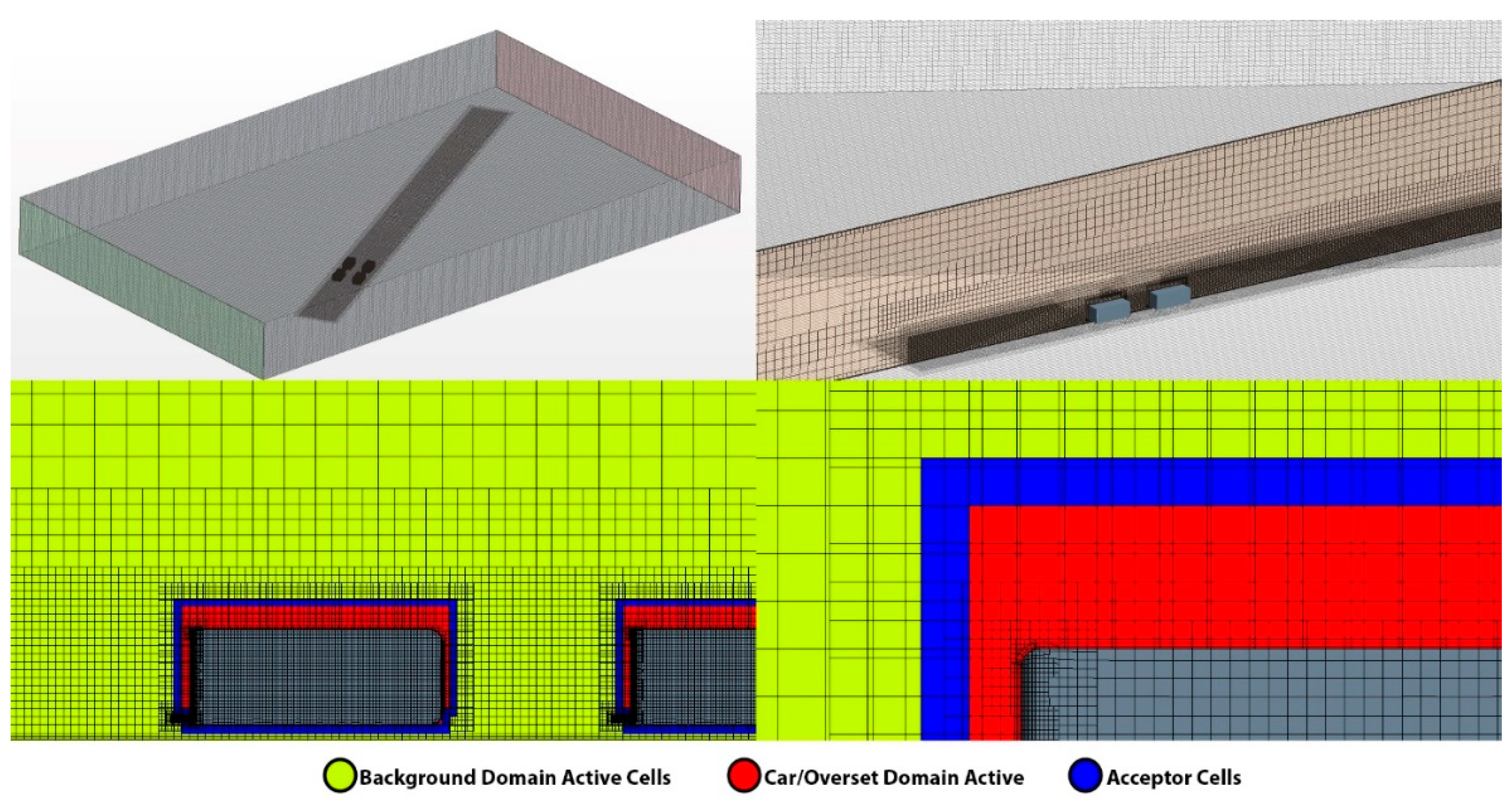
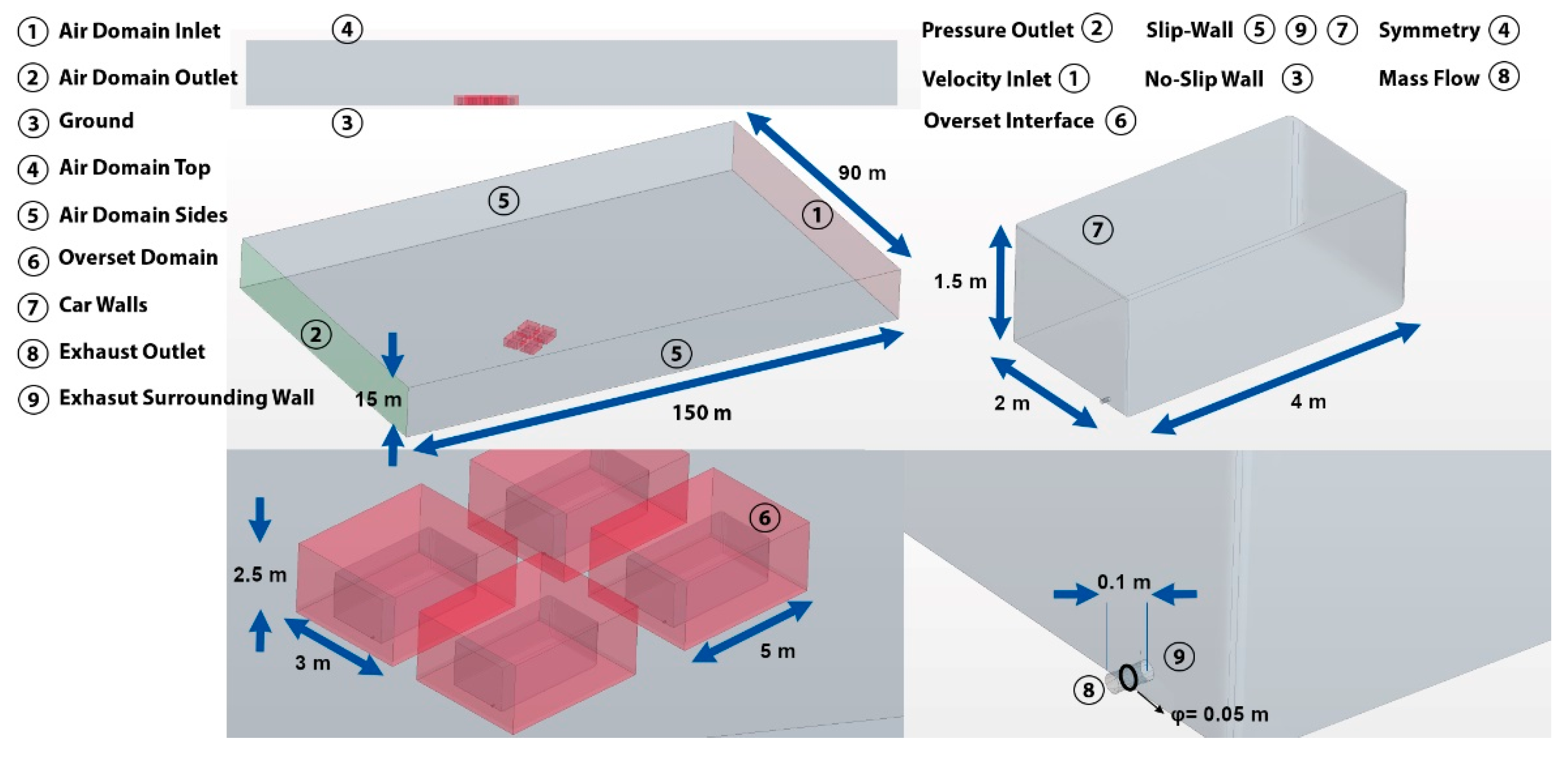
2. Methodology
3. Results and Discussion
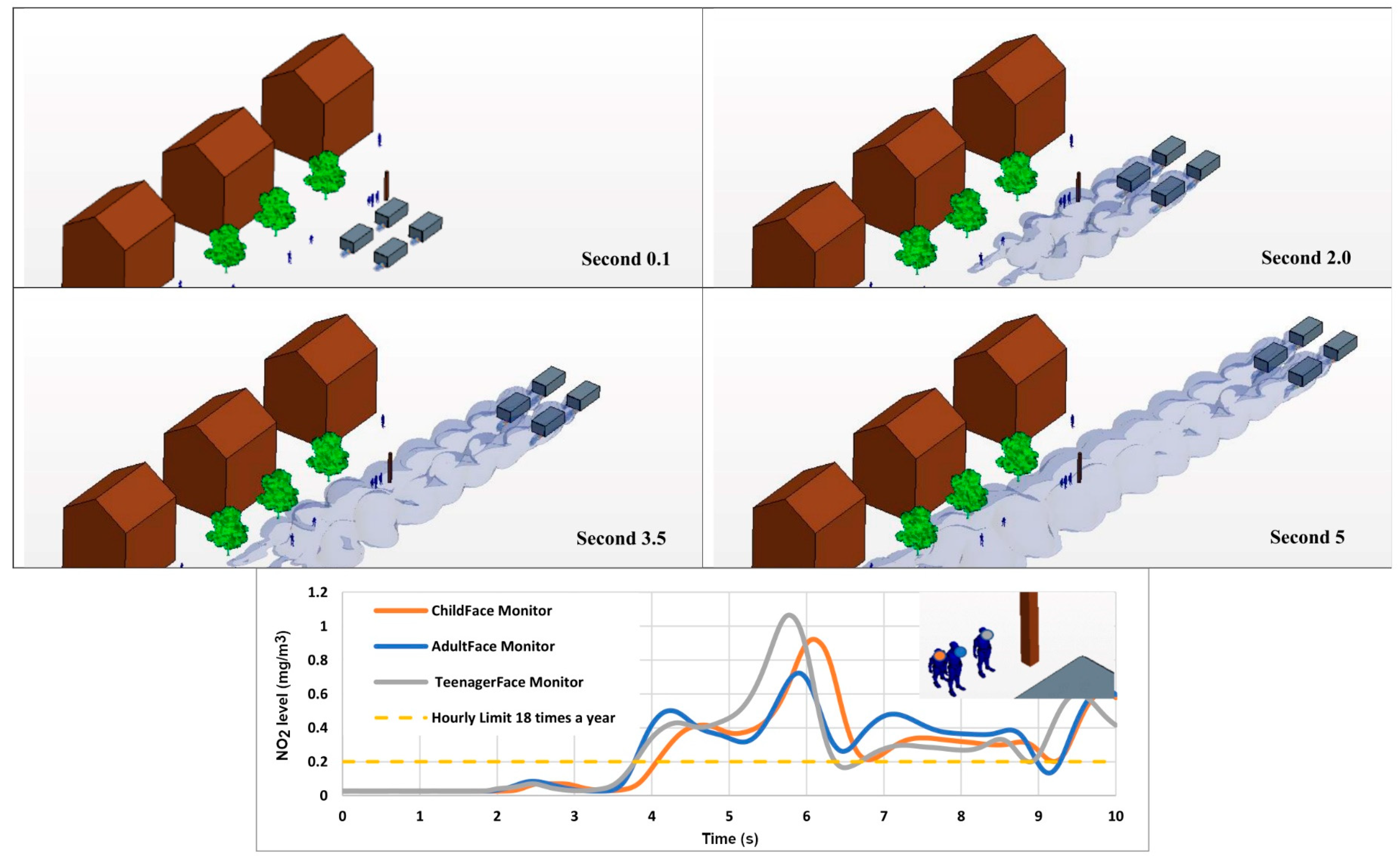
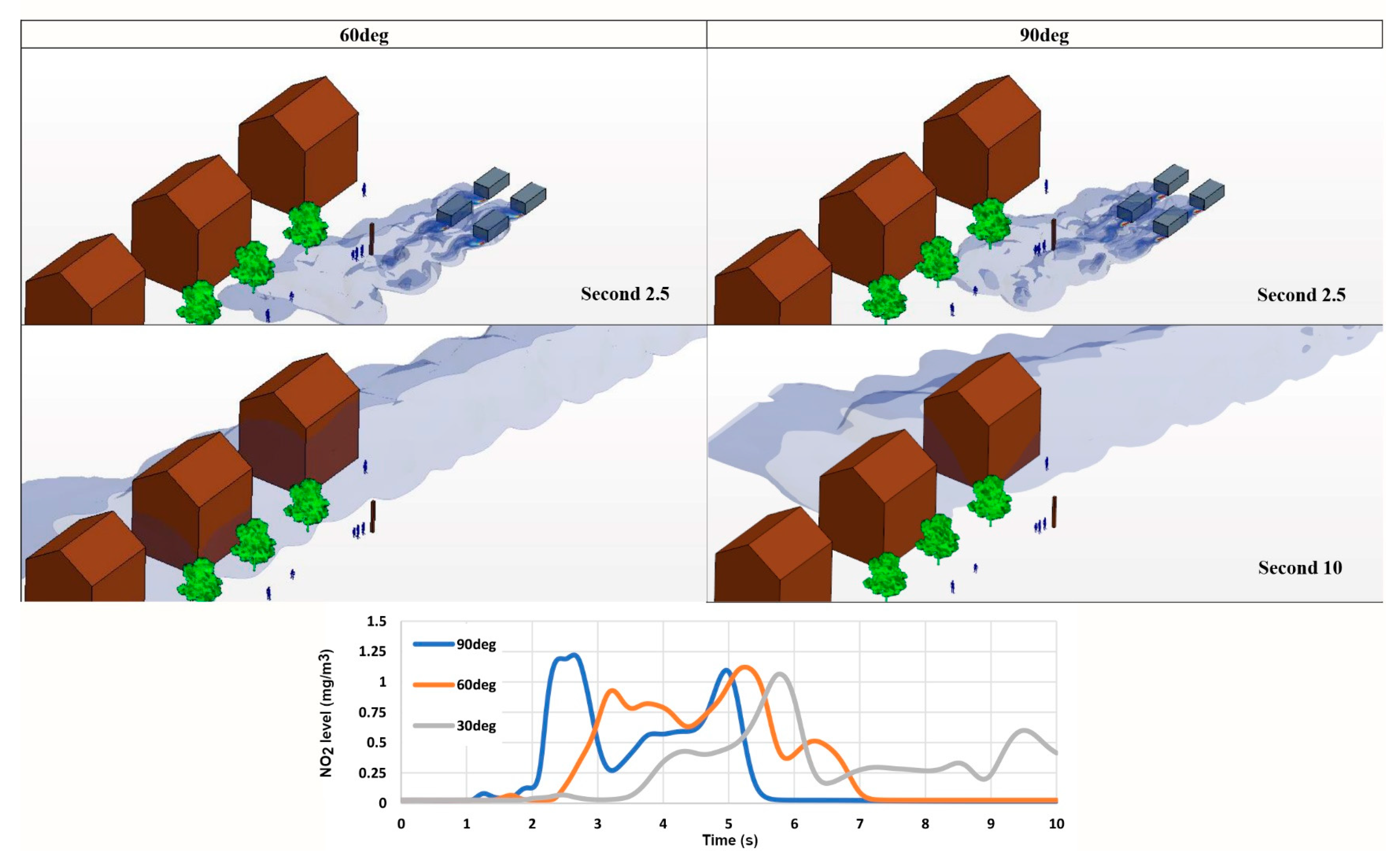
3.1. Case 1. Baseline Model: Demonstration of Personal Exposure and Effects of Wind Direction
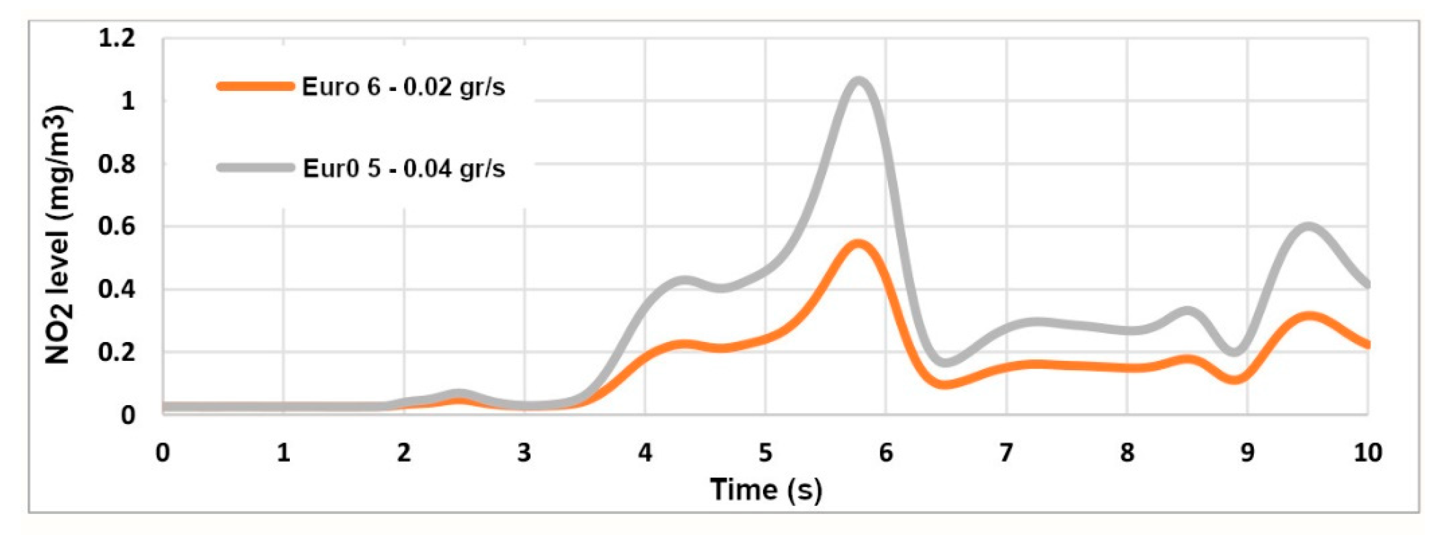
3.2. Case 2. Personal Exposure from Euro 6-Rated Vehicles
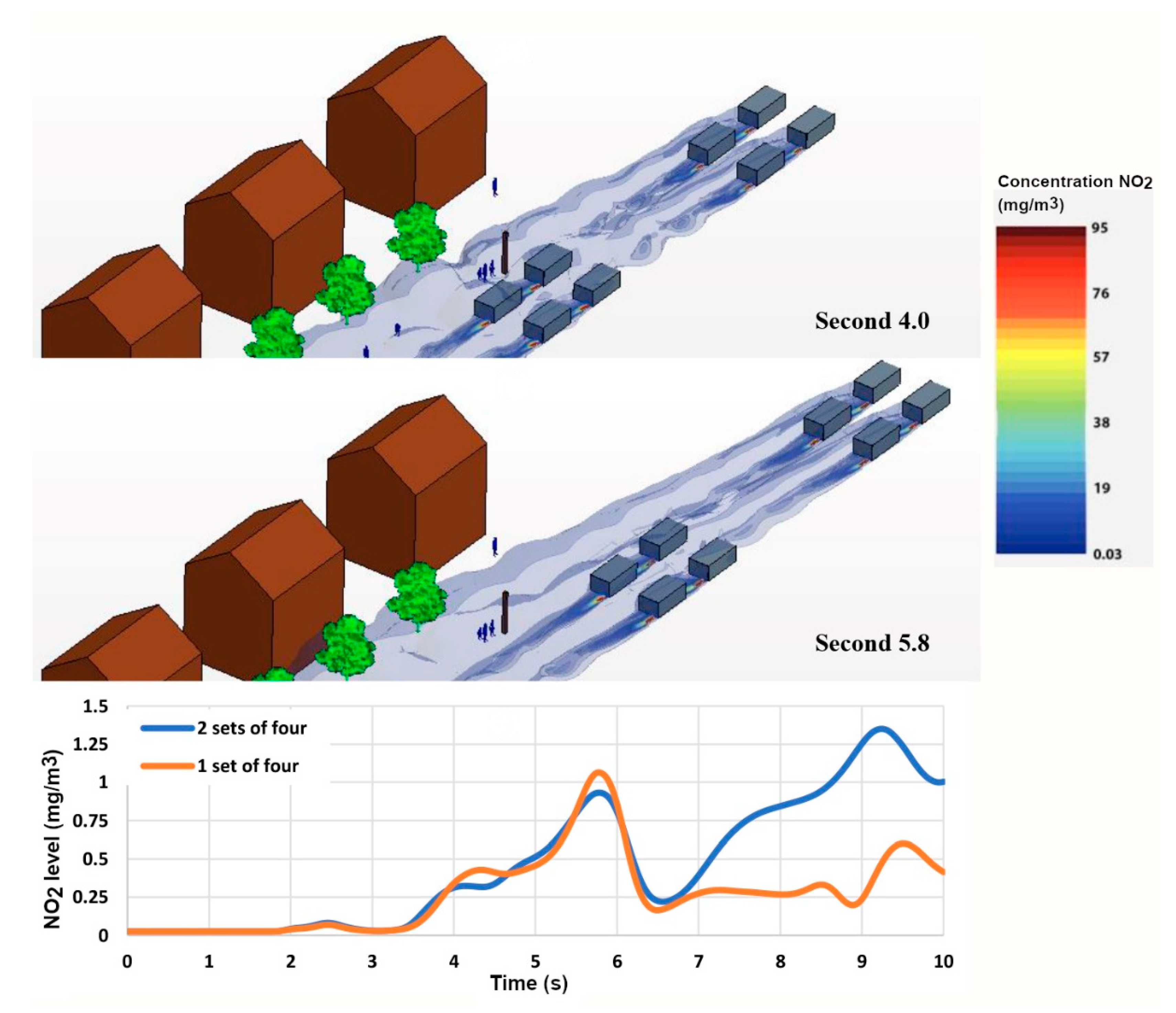
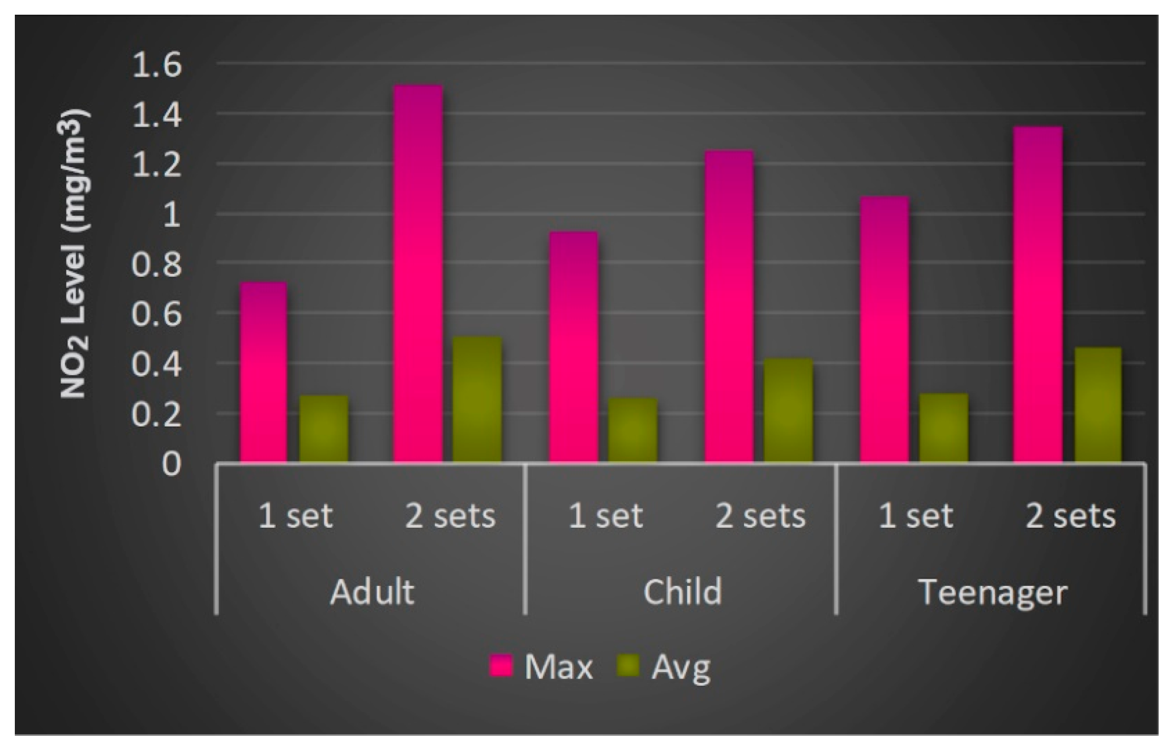
3.3. Case 3. Increase in Exposure Due to Localised Pollutants Accumulation (8-Vehicle Model)
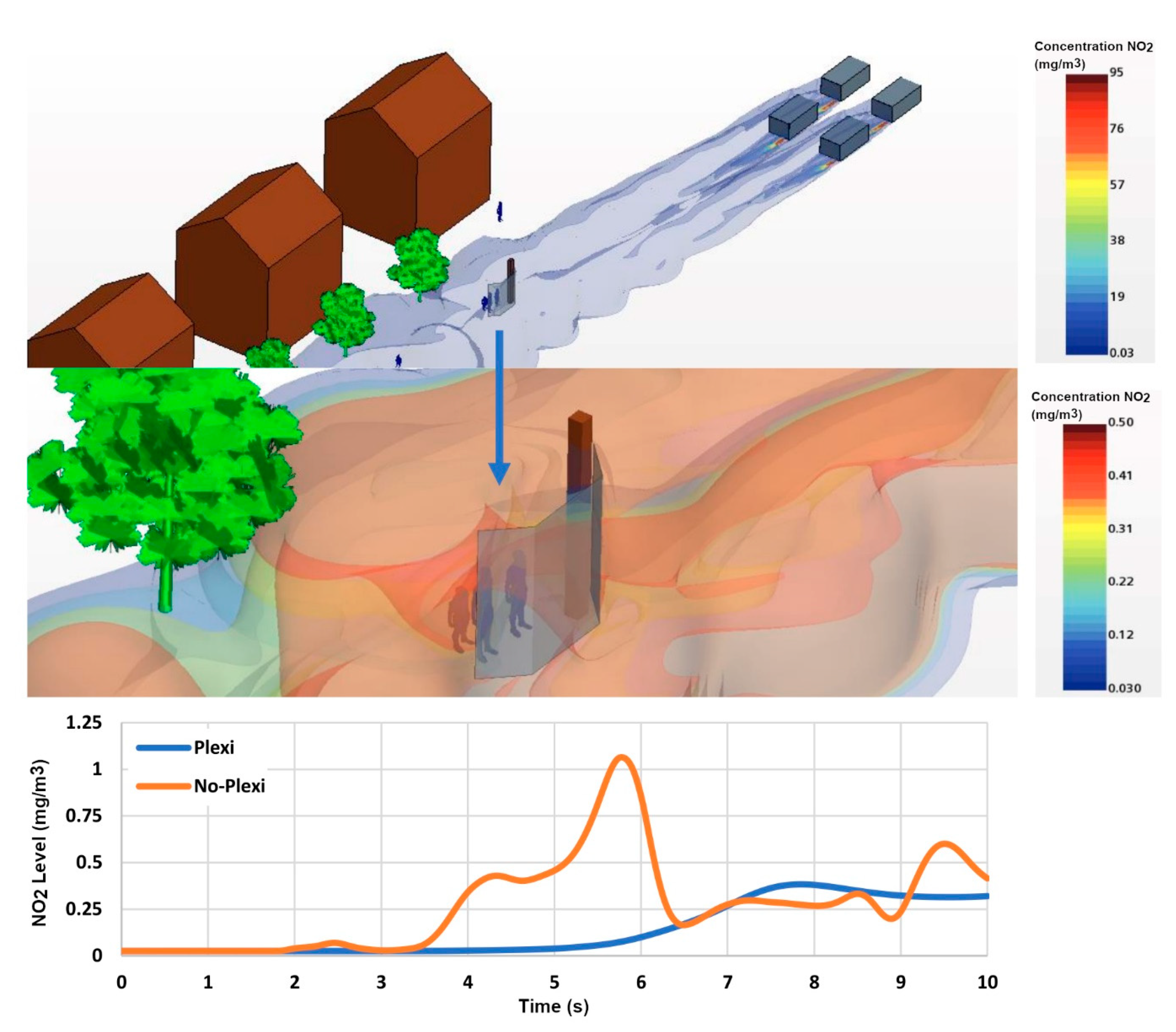
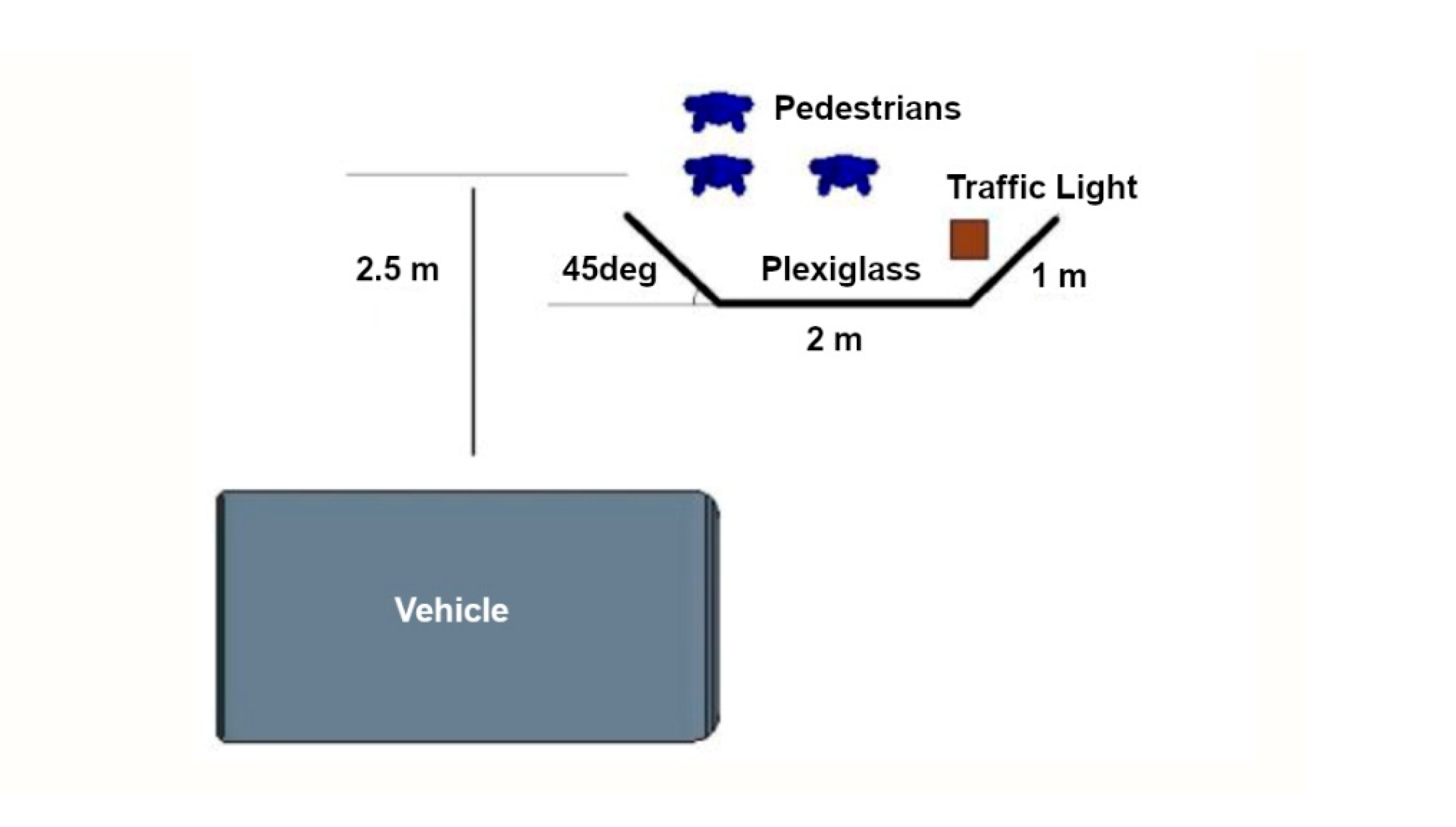
3.4. Case 4. Effect of Potential Intervention Measures
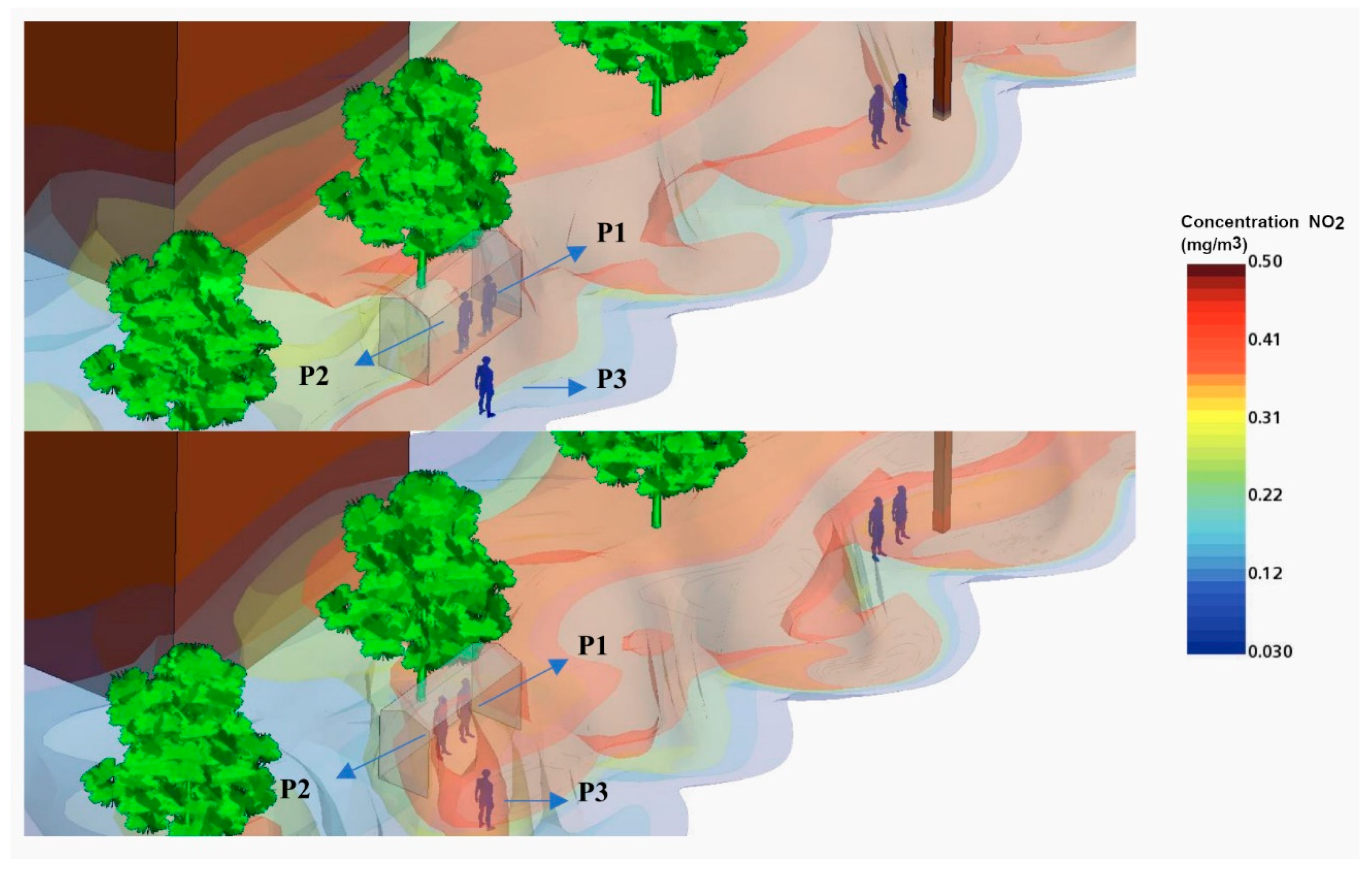
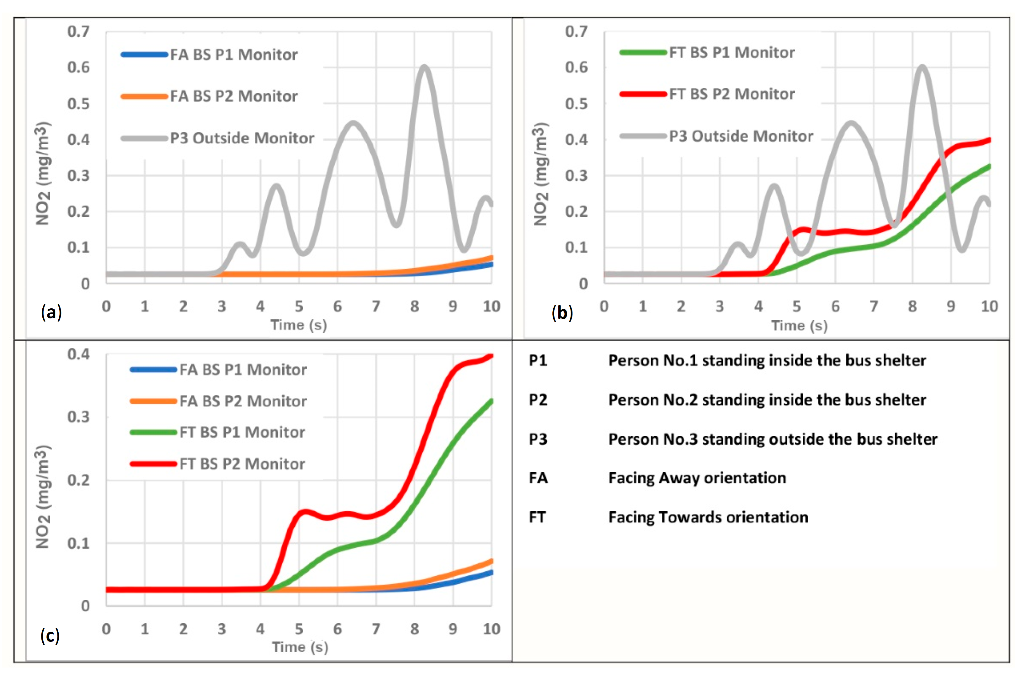
3.5. Case 5. Bus Shelters
4. Conclusions
Author Contributions
Funding
Institutional Review Board Statement
Informed Consent Statement
Data Availability Statement
Conflicts of Interest
References
- World Health Organization. Review of Evidence on Health Aspects of Air Pollution: REVIHAAP Project: Technical Report; World Health Organization Regional Office for Europe: Copenhagen, Denmark, 2021. [Google Scholar]
- Andersen, Z.J.; Loft, S.; Ketzel, M.; Stage, M.; Scheike, T.; Hermansen, M.N.; Bisgaard, H. Ambient air pollution triggers wheezing symptoms in infants. Thorax 2008, 63, 710–716. [Google Scholar] [CrossRef] [PubMed] [Green Version]
- Escamilla-Nuñez, M.-C.; Barraza-Villarreal, A.; Hernandez-Cadena, L.; Moreno-Macias, H.; Ramirez-Aguilar, M.; Sienra-Monge, J.-J.; Cortez-Lugo, M.; Texcalac, J.-L.; del Rio-Navarro, B.; Romieu, I. Traffic-related air pollution and respiratory symptoms among asthmatic children, resident in Mexico City: The EVA cohort study. Respir. Res. 2008, 9, 1–11. [Google Scholar] [CrossRef] [PubMed] [Green Version]
- Faustini, A.; Stafoggia, M.; Cappai, G.; Forastiere, F. Short-term effects of air pollution in a cohort of patients with chronic obstructive pulmonary disease. Epidemiology 2012, 23, 861–879. [Google Scholar] [CrossRef] [PubMed]
- Chen, R.; Wang, X.; Meng, X.; Hua, J.; Zhou, Z.; Chen, B.; Kan, H. Communicating air pollution-related health risks to the public: An application of the Air Quality Health Index in Shanghai, China. Environ. Int. 2013, 51, 168–173. [Google Scholar] [CrossRef]
- Schultz, E.S.; Gruzieva, O.; Bellander, T.; Bottai, M.; Hallberg, J.; Kull, I.; Svartengren, M.; Melén, E.; Pershagen, G. Traffic-related air pollution and lung function in children at 8 years of age: A birth cohort study. Am. J. Respir. Crit. Care Med. 2012, 186, 1286–1291. [Google Scholar] [CrossRef] [Green Version]
- Anderson, G.B.; Krall, J.R.; Peng, R.D.; Bell, M.L. Is the relation between ozone and mortality confounded by chemical components of particulate matter? Analysis of 7 components in 57 US communities. Am. J. Epidemiol. 2012, 176, 726–732. [Google Scholar] [CrossRef] [Green Version]
- Gruzieva, O.; Bergström, A.; Hulchiy, O.; Kull, I.; Lind, T.; Melén, E.; Moskalenko, V.; Pershagen, G.; Bellander, T. Exposure to air pollution from traffic and childhood asthma until 12 years of age. Epidemiology 2013, 24, 54–61. [Google Scholar] [CrossRef]
- Sanchez, B.; Santiago, J.L.; Martilli, A.; Palacios, M.; Núñez, L.; Pujadas, M.; Fernández-Pampillón, J. NOx depolluting performance of photocatalytic materials in an urban area—Part II: Assessment through Computational Fluid Dynamics simulations. Atmos. Environ. 2021, 246, 118091. [Google Scholar] [CrossRef]
- Gehring, U.; Heinrich, J.; Krämer, U.; Grote, V.; Hochadel, M.; Sugiri, D.; Kraft, M.; Rauchfuss, K.; Eberwein, H.G.; Wichmann, H.E. Long-term exposure to ambient air pollution and cardiopulmonary mortality in women. Epidemiology 2006, 17, 545–551. [Google Scholar] [CrossRef]
- Hoffmann, B.; Moebus, S.; Stang, A.; Beck, E.M.; Dragano, N.; Möhlenkamp, S.; Schmermund, A.; Memmesheimer, M.; Mann, K.; Erbel, R.; et al. Residence close to high traffic and prevalence of coronary heart disease. Eur. Heart J. 2006, 27, 2696–2702. [Google Scholar] [CrossRef] [Green Version]
- Morgenstern, V.; Zutavern, A.; Cyrys, J.; Brockow, I.; Gehring, U.; Koletzko, S.; Bauer, C.P.; Reinhardt, D.; Wichmann, H.E.; Heinrich, J. Respiratory health and individual estimated exposure to traffic-related air pollutants in a cohort of young children. Occup. Environ. Med. 2007, 64, 8–16. [Google Scholar] [CrossRef] [PubMed] [Green Version]
- Morgenstern, V.; Zutavern, A.; Cyrys, J.; Brockow, I.; Koletzko, S.; Krämer, U.; Behrendt, H.; Herbarth, O.; von Berg, A.; Bauer, C.P.; et al. Atopic diseases, allergic sensitization, and exposure to traffic-related air pollution in children. Am. J. Respir. Crit. Care Med. 2008, 177, 1331–1337. [Google Scholar] [CrossRef] [PubMed]
- Gordian, M.E.; Haneuse, S.; Wakefield, J. An investigation of the association between traffic exposure and the diagnosis of asthma in children. J. Expo. Sci. Environ. Epidemiol. 2006, 16, 49–55. [Google Scholar] [CrossRef] [PubMed]
- Kim, J.J.; Huen, K.; Adams, S.; Smorodinsky, S.; Hoats, A.; Malig, B.; Lipsett, M.; Ostro, B. Residential traffic and children’s respiratory health. Environ. Health Perspect 2008, 116, 1274–1279. [Google Scholar] [CrossRef] [PubMed] [Green Version]
- Karner, A.A.; Eisinger, D.S.; Niemeier, D.A. Near-Roadway Air Quality: Synthesizing the Findings from Real-World Data. Environ. Sci. Technol. 2010, 44, 5334–5344. [Google Scholar] [CrossRef]
- Peachey, C.J.; Sinnett, D.; Wilkinson, M.; Morgan, G.W.; Freer-Smith, P.H.; Hutchings, T.R. Deposition and solubility of airborne metals to four plant species grown at varying distances from two heavily trafficked roads in London. Environ. Pollut. 2009, 157, 2291–2299. [Google Scholar] [CrossRef] [Green Version]
- Davison, J.; Rose, R.A.; Farren, N.J.; Wagner, R.L.; Murrells, T.P.; Carslaw, D.C. Verification of a National Emission Inventory and Influence of On-road Vehicle Manufacturer-Level Emissions. Environ. Sci. Technol. 2021, 55, 4452–4461. [Google Scholar] [CrossRef]
- EEA. Air Quality in Europe-2016 Report; Publications Office of the European Union: Luxembourg, 2016.
- NAEI. Pollutant Information: Nitrogen Oxides; National Atmospheric Emissions Inventory: London, UK, 2018.
- Elliot, A.J.; Smith, S.; Dobney, A.; Thornes, J.; Smith, G.E.; Vardoulakis, S. Monitoring the effect of air pollution episodes on health care consultations and ambulance call-outs in England during March/April 2014: A retrospective observational analysis. Environ. Pollut. 2016, 214, 903–911. [Google Scholar] [CrossRef] [Green Version]
- Santiago, J.L.; Borge, R.; Sanchez, B.; Quaassdorff, C.; de la Paz, D.; Martilli, A.; Rivas, E.; Martín, F. Estimates of pedestrian exposure to atmospheric pollution using high-resolution modelling in a real traffic hot-spot. Sci. Total Environ. 2021, 755, 142475. [Google Scholar] [CrossRef]
- Yatkin, S.; Gerboles, M.; Belis, C.A.; Karagulian, F.; Lagler, F.; Barbiere, M.; Borowiak, A. Representativeness of an air quality monitoring station for PM2.5 and source apportionment over a small urban domain. Atmos. Pollut. Res. 2020, 11, 225–233. [Google Scholar] [CrossRef]
- Song, X.; Zhao, Y. Numerical investigation of airflow patterns and pollutant dispersions induced by a fleet of vehicles inside road tunnels using dynamic mesh part Ⅰ: Traffic wind evaluation. Atmos. Environ. 2019, 212, 208–220. [Google Scholar] [CrossRef]
- Xing, Y.; Brimblecombe, P. Role of vegetation in deposition and dispersion of air pollution in urban parks. Atmos. Environ. 2019, 201, 73–83. [Google Scholar] [CrossRef]
- Martín, F.; Santiago, J.L.; Kracht, O.; García, L.; Gerboles, M. FAIRMODE Spatial Representativeness Feasibility Study; Report EUR 27385; Publications Office of the European Union: Luxembourg, 2015.
- Sanchez, B.; Santiago, J.L.; Martilli, A.; Martin, F.; Borge, R.; Quaassdorff, C.; de la Paz, D. Modelling NOX concentrations through CFD-RANS in an urban hot-spot using high resolution traffic emissions and meteorology from a mesoscale model. Atmos. Environ. 2017, 163, 155–165. [Google Scholar] [CrossRef]
- Woodward, H.; Stettler, M.; Pavlidis, D.; Aristodemou, E.; ApSimon, H.; Pain, C. A large eddy simulation of the dispersion of traffic emissions by moving vehicles at an intersection. Atmos. Environ. 2019, 215, 116891. [Google Scholar] [CrossRef]
- Hess, D.B.; Ray, P.D.; Stinson, A.E.; Park, J. Determinants of exposure to fine particulate matter (PM2.5) for waiting passengers at bus stops. Atmos. Environ. 2010, 44, 5174–5182. [Google Scholar] [CrossRef]
- Moore, A.; Figliozzi, M.; Monsere, C.M. Air quality at bus stops: Empirical analysis of exposure to particulate matter at bus stop shelters. Transp. Res. Rec. 2012, 2270, 76–86. [Google Scholar] [CrossRef] [Green Version]
- Jeanjean, A.P.R.; Gallagher, J.; Monks, P.S.; Leigh, R.J. Ranking current and prospective NO2 pollution mitigation strategies: An environmental and economic modelling investigation in Oxford Street, London. Environ. Pollut. 2017, 225, 587–597. [Google Scholar] [CrossRef] [Green Version]
- Buccolieri, R.; Santiago, J.-L.; Rivas, E.; Sanchez, B. Review on urban tree modelling in CFD simulations: Aerodynamic, deposition and thermal effects. Urban For. Urban Green. 2018, 31, 212–220. [Google Scholar] [CrossRef]
- Abhijith, K.V.; Kumar, P.; Gallagher, J.; McNabola, A.; Baldauf, R.; Pilla, F.; Broderick, B.; Di Sabatino, S.; Pulvirenti, B. Air pollution abatement performances of green infrastructure in open road and built-up street canyon environments—A review. Atmos. Environ. 2017, 162, 71–86. [Google Scholar] [CrossRef]
- Al-Dabbous, A.N.; Kumar, P. The influence of roadside vegetation barriers on airborne nanoparticles and pedestrians exposure under varying wind conditions. Atmos. Environ. 2014, 90, 113–124. [Google Scholar] [CrossRef] [Green Version]
- Santiago, J.-L.; Buccolieri, R.; Rivas, E.; Calvete-Sogo, H.; Sanchez, B.; Martilli, A.; Alonso, R.; Elustondo, D.; Santamaría, J.M.; Martin, F. CFD modelling of vegetation barrier effects on the reduction of traffic-related pollutant concentration in an avenue of Pamplona, Spain. Sustain. Cities Soc. 2019, 48, 101559. [Google Scholar] [CrossRef]
- Jia, Y.-P.; Lu, K.-F.; Zheng, T.; Li, X.-B.; Liu, X.; Peng, Z.-R.; He, H.-D. Effects of roadside green infrastructure on particle exposure: A focus on cyclists and pedestrians on pathways between urban roads and vegetative barriers. Atmos. Pollut. Res. 2021, 12, 1–12. [Google Scholar] [CrossRef]
- Hu, M.; Wang, Y.; Wang, S.; Jiao, M.; Huang, G.; Xia, B. Spatial-temporal heterogeneity of air pollution and its relationship with meteorological factors in the Pearl River Delta, China. Atmos. Environ. 2021, 254, 118415. [Google Scholar] [CrossRef]
- Borge, R.; Narros, A.; Artíñano, B.; Yagüe, C.; Gómez-Moreno, F.J.; de la Paz, D.; Román-Cascón, C.; Díaz, E.; Maqueda, G.; Sastre, M.; et al. Assessment of microscale spatio-temporal variation of air pollution at an urban hotspot in Madrid (Spain) through an extensive field campaign. Atmos. Environ. 2016, 140, 432–445. [Google Scholar] [CrossRef]
- Lauriks, T.; Longo, R.; Baetens, D.; Derudi, M.; Parente, A.; Bellemans, A.; van Beeck, J.; Denys, S. Application of Improved CFD Modeling for Prediction and Mitigation of Traffic-Related Air Pollution Hotspots in a Realistic Urban Street. Atmos. Environ. 2021, 246, 118127. [Google Scholar] [CrossRef]
- Jeanjean, A.P.R.; Monks, P.S.; Leigh, R.J. Modelling the effectiveness of urban trees and grass on PM2.5 reduction via dispersion and deposition at a city scale. Atmos. Environ. 2016, 147, 1–10. [Google Scholar] [CrossRef] [Green Version]
- Mei, S.-J.; Luo, Z.; Zhao, F.-Y.; Wang, H.-Q. Street canyon ventilation and airborne pollutant dispersion: 2-D versus 3-D CFD simulations. Sustain. Cities Soc. 2019, 50, 101700. [Google Scholar] [CrossRef]
- STAR-CCM+ User Guide. 2020. Available online: https://community.sw.siemens.com/s/question/0D54O000061xpUOSAY/starccm-user-guide-tutorials-knowledge-base-and-tech-support (accessed on 22 March 2022).
- Quality, O.A. Oxfordshire AirQuality Website. Available online: https://oxfordshire.air-quality.info/ (accessed on 22 May 2022).
- Costagliola, M.A.; Costabile, M.; Prati, M.V. Impact of road grade on real driving emissions from two Euro 5 diesel vehicles. Appl. Energy 2018, 231, 586–593. [Google Scholar] [CrossRef]
- Söderena, P.; Laurikko, J.; Weber, C.; Tilli, A.; Kuikka, K.; Kousa, A.; Väkevä, O.; Venho, A.; Haaparanta, S.; Nuottimäki, J. Monitoring Euro 6 diesel passenger cars NOx emissions for one year in various ambient conditions with PEMS and NOx sensors. Sci. Total Environ. 2020, 746, 140971. [Google Scholar] [CrossRef]
- Merker, G.P.; Teichmann, R. Grundlagen Verbrennungsmotoren: Funktionsweise, Simulation, Messtechnik; Springer: Berlin/Heidelberg, Germany, 2014. [Google Scholar]
- World Health Organization. Ambient (Outdoor) Air Quality and Health. Available online: https://www.who.int/news-room/fact-sheets/detail/ambient-(outdoor)-air-quality-and-health (accessed on 22 May 2022).
- Department for Environment Food & Rural Affairs. Concentrations of Nitrogen Dioxide. Available online: https://www.gov.uk/government/statistics/air-quality-statistics/ntrogen-dioxide (accessed on 22 May 2022).
- Rivas, E.; Santiago, J.L.; Lechón, Y.; Martín, F.; Ariño, A.; Pons, J.J.; Santamaría, J.M. CFD modelling of air quality in Pamplona City (Spain): Assessment, stations spatial representativeness and health impacts valuation. Sci. Total Environ. 2019, 649, 1362–1380. [Google Scholar] [CrossRef]


| Case No. | Number of Vehicles | NOx Emission Rate per Vehicle (as NO2 Equivalent) | Wind Angle (deg) | Mitigation Measure |
|---|---|---|---|---|
| 1 | 4 | 0.04 g/s Euro 5, [44] | 30/60/90 | N/A |
| 2 | 4 | 0.02 g/s Euro 6, [45] | 30 | |
| 3 | 8 | 0.04 g/s Euro 5, [44] | ||
| 4 | 4 | Plexiglass barrier by the traffic light | ||
| 5 | 4 | Bus stop shelter facing towards/away the road |
| Gas Component | Mass Fraction % |
|---|---|
| NO2 | 0.142 |
| O2 | 15 |
| H2O | 2.6 |
| CO2 | 7.2 |
| N2 | 75.058 |
Publisher’s Note: MDPI stays neutral with regard to jurisdictional claims in published maps and institutional affiliations. |
© 2022 by the authors. Licensee MDPI, Basel, Switzerland. This article is an open access article distributed under the terms and conditions of the Creative Commons Attribution (CC BY) license (https://creativecommons.org/licenses/by/4.0/).
Share and Cite
Tajdaran, S.; Bonatesta, F.; Mason, B.; Morrey, D. Simulation of Traffic-Born Pollutant Dispersion and Personal Exposure Using High-Resolution Computational Fluid Dynamics. Environments 2022, 9, 67. https://doi.org/10.3390/environments9060067
Tajdaran S, Bonatesta F, Mason B, Morrey D. Simulation of Traffic-Born Pollutant Dispersion and Personal Exposure Using High-Resolution Computational Fluid Dynamics. Environments. 2022; 9(6):67. https://doi.org/10.3390/environments9060067
Chicago/Turabian StyleTajdaran, Sadjad, Fabrizio Bonatesta, Byron Mason, and Denise Morrey. 2022. "Simulation of Traffic-Born Pollutant Dispersion and Personal Exposure Using High-Resolution Computational Fluid Dynamics" Environments 9, no. 6: 67. https://doi.org/10.3390/environments9060067
APA StyleTajdaran, S., Bonatesta, F., Mason, B., & Morrey, D. (2022). Simulation of Traffic-Born Pollutant Dispersion and Personal Exposure Using High-Resolution Computational Fluid Dynamics. Environments, 9(6), 67. https://doi.org/10.3390/environments9060067