
Atmospheric Contamination of Coastal Cities by the Exhaust Emissions of Docked Marine Vessels: The Case of Tromsø


Abstract
:1. Introduction
2. Materials and Methods
2.1. Computational Fluid Dynamics
2.2. Atmospheric Boundary Layer
2.3. Numerical Solutions
3. Results
3.1. Simulation Run
3.2. Wind Direction
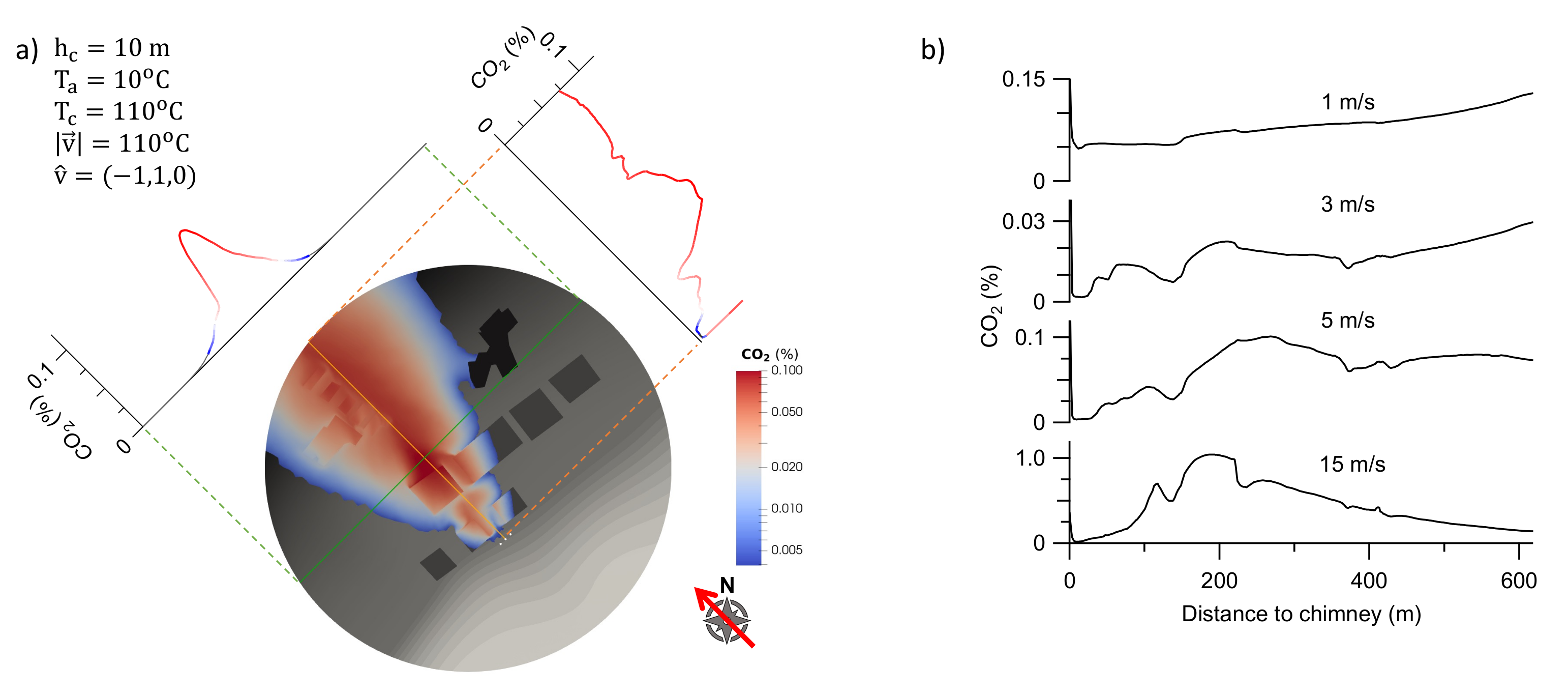
3.3. Wind Speed
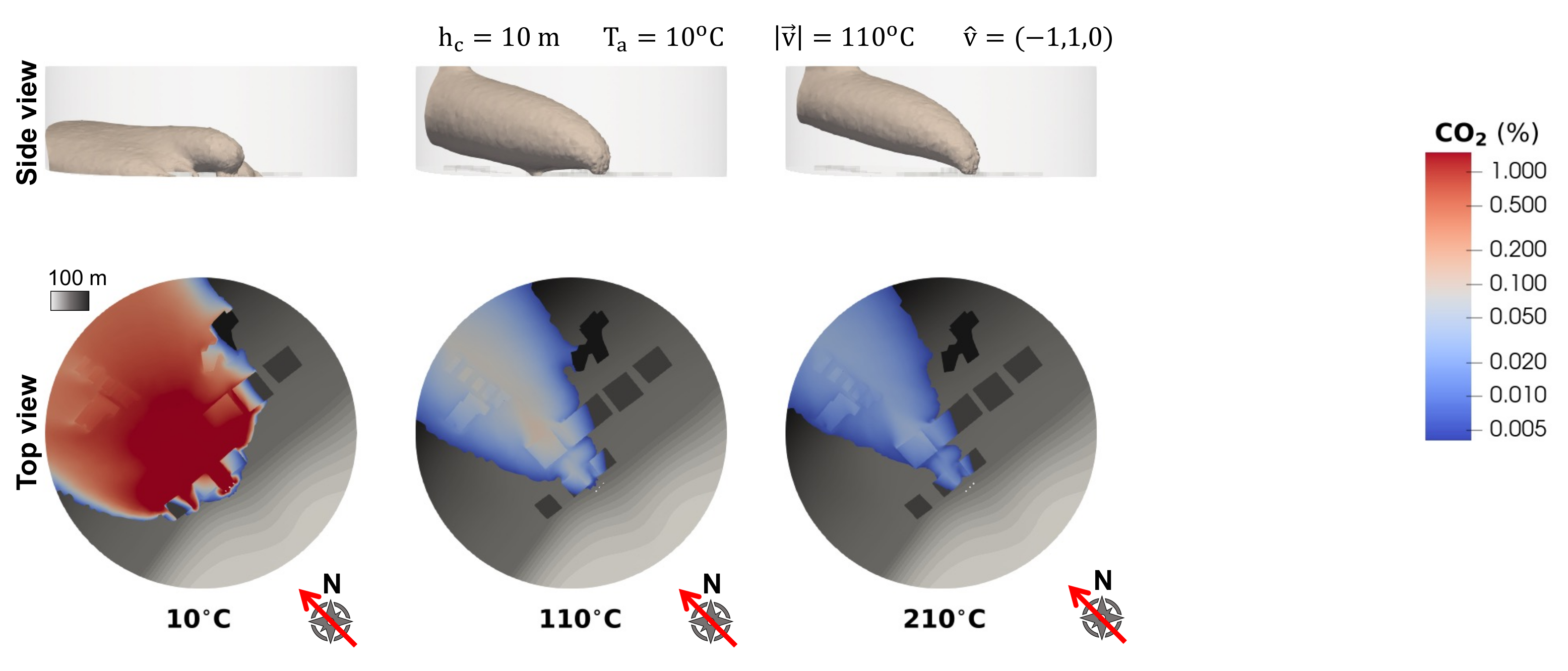
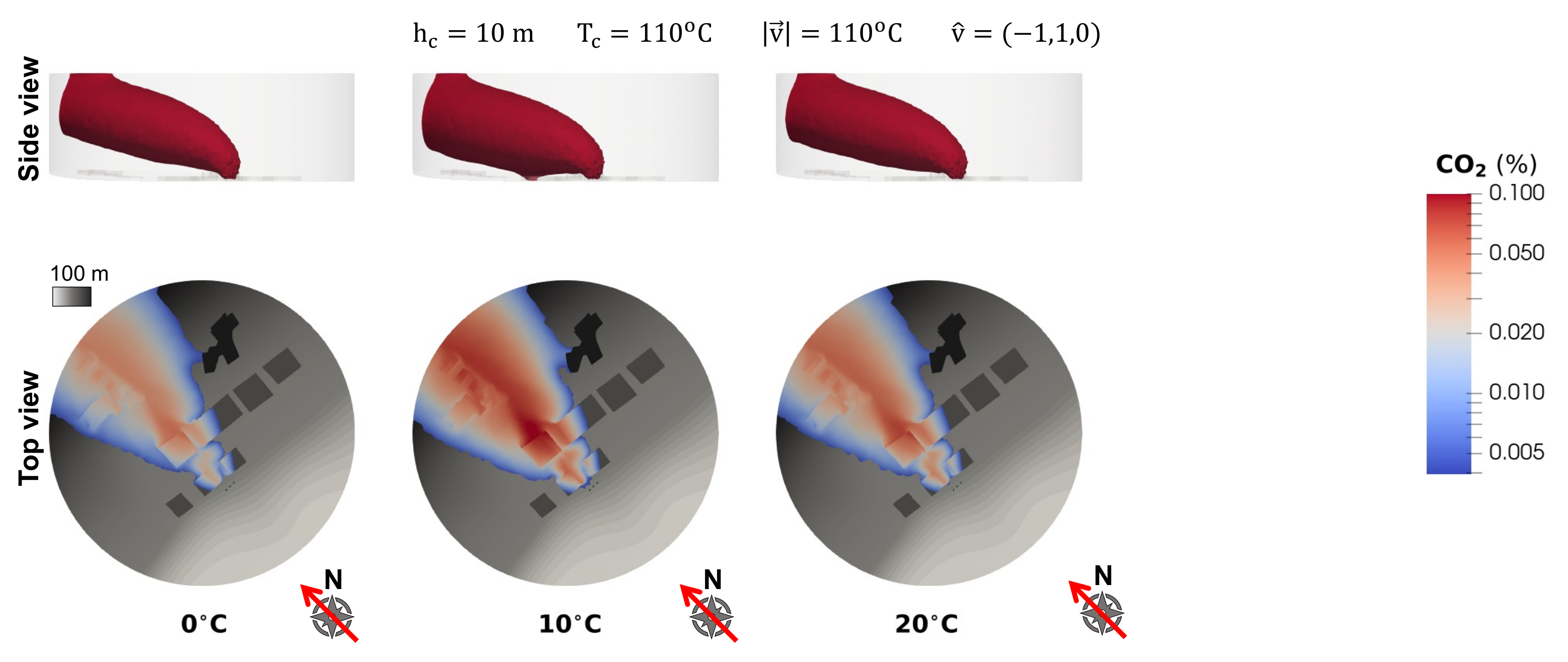
3.4. Temperature of the Plume
3.5. Chimney Height
4. Discussion
5. Conclusions
Author Contributions
Funding
Conflicts of Interest
References
- Kim, K.H.; Kabir, E.; Kabir, S. A review on the human health impact of airborne particulate matter. Environ. Int. 2015, 74, 136–143. [Google Scholar] [CrossRef] [PubMed]
- Davidson, C.I.; Phalen, R.F.; Solomon, P.A. Airborne Particulate Matter and Human Health: A Review. Aerosol Sci. Technol. 2005, 39, 737–749. [Google Scholar] [CrossRef]
- Roskilly, A.P.; Nanda, S.K.; Wang, Y.D.; Chirkowski, J. The performance and the gaseous emissions of two small marine craft diesel engines fuelled with biodiesel. Appl. Therm. Eng. 2008, 28, 872–880. [Google Scholar] [CrossRef]
- Walter, R.A.; Broderick, A.J.; Sturm, J.C.; Klaubert, E.C. USCG Pollution Abatement Program: A Preliminary Study of Vessel and Boat Exhaust Emissions; Report Number DOT-TSC-USCG-72-3; United States Coast Guard: Washington, DC, USA; John A. Volpe National Transportation Systems Center: Cambridge, MA, USA, 1971.
- Simeone, L.F. The Intrusion of Engine Exhaust into the Passenger Areas of Recreational Power Boats; Report Number, 227783325; United States Coast Guard: Washington, DC, USA; John A. Volpe National Transportation Systems Center: Cambridge, MA, USA, 1991.
- Bentz, A.P.; Weaver, E. Marine Diesel Exhaust Emissions Measured by Portable Instruments. SAE Trans. 1994, 103, 1872–1876. [Google Scholar]
- Johansson, L.; Ytreberg, E.; Jalkanen, J.P.; Fridell, E.; Eriksson, K.M.; Lagerström, M.; Maljutenko, I.; Raudsepp, U.; Fischer, V.; Roth, E. Model for leisure boat activities and emissions—Implementation for the Baltic Sea. Ocean Sci. 2020, 16, 1143–1163. [Google Scholar] [CrossRef]
- Schleijpen, H.M.A.; Neele, F.P. Ship exhaust gas plume cooling. In Proceedings of the SPIE Conference—Targets and Backgrounds X: Characterization and Representation, Orlando, FL, USA, 12–16 April 2004; 5431, pp. 66–76. [Google Scholar] [CrossRef] [Green Version]
- Garcia-Gonzales, D.A.; Shamasunder, B.; Jerrett, M. Distance decay gradients in hazardous air pollution concentrations around oil and natural gas facilities in the city of Los Angeles: A pilot study. Environ. Res. 2019, 173, 232–236. [Google Scholar] [CrossRef] [PubMed]
- Ran, L.; Lin, W.L.; Deji, Y.Z.; La, B.; Tsering, P.M.; Xu, X.B.; Wang, W. Surface gas pollutants in Lhasa, a highland city of Tibet; current levels and pollution implications. Atmos. Chem. Phys. 2014, 14, 10721–10730. [Google Scholar] [CrossRef] [Green Version]
- Zhang, R.; Wang, G.; Guo, S.; Zamora, M.L.; Ying, Q.; Lin, Y.; Wang, W.; Hu, M.; Wang, Y. Formation of Urban Fine Particulate Matter. Chem. Rev. 2015, 115, 3803–3855. [Google Scholar] [CrossRef] [PubMed]
- Gorelick, N.; Hancher, M.; Dixon, M.; Ilyushchenko, S.; Thau, D.; Moore, R. Google Earth Engine: Planetary-scale geospatial analysis for everyone. Remote Sens. Environ. 2017, 202, 18–27. [Google Scholar] [CrossRef]
- Solidworks® 26; Dassault Systèmes SolidWorks Corporation: Paris, France, 2018.
- Ansys® Workbench 18; ANSYS Inc.: Canonsburg, PA, USA, 2018.
- Launder, B.E.; Spalding, D.B. The numerical computation of turbulent flows. Comput. Methods Appl. Mech. Eng. 1974, 3, 269–289. [Google Scholar] [CrossRef]
- Richards, P.J.; Hoxey, R.P. Appropriate boundary conditions for computational wind engineering models using the k-ϵ turbulence model. J. Wind. Eng. Ind. Aerodyn. 1993, 46–47, 145–153. [Google Scholar] [CrossRef]
- Hargreaves, D.M.; Wright, N.G. On the use of the k–ϵ model in commercial CFD software to model the neutral atmospheric boundary layer. J. Wind. Eng. Ind. Aerodyn. 2007, 95, 355–369. [Google Scholar] [CrossRef]
- Yang, Y.; Gu, M.; Chen, S.; Jin, X. New inflow boundary conditions for modelling the neutral equilibrium atmospheric boundary layer in computational wind engineering. J. Wind. Eng. Ind. Aerodyn. 2009, 97, 88–95. [Google Scholar] [CrossRef]
- Weller, H.G.; Tabor, G.; Jasak, H.; Fureby, C. A tensorial approach to computational continuum mechanics using object-oriented techniques. Comput. Phys. 1998, 12, 620–631. [Google Scholar] [CrossRef]
- Issa, R.I. Solution of the implicitly discretised fluid flow equations by operator-splitting. J. Comput. Phys. 1986, 62, 40–65. [Google Scholar] [CrossRef]
- Caretto, L.S.; Gosman, A.D.; Patankar, S.V.; Spalding, D.B. Two calculation procedures for steady, three-dimensional flows with recirculation. In Proceedings of the Third International Conference on Numerical Methods in Fluid Mechanics; Lecture Notes in Physics. Cabannes, H., Temam, R., Eds.; Springer: Berlin/Heidelberg, Germany, 1973; pp. 60–68. [Google Scholar] [CrossRef]
- Garratt, J.R. Review: The atmospheric boundary layer. Earth-Sci. Rev. 1994, 37, 89–134. [Google Scholar] [CrossRef]
- Tran, V.; Ng, E.Y.K.; Skote, M. CFD simulation of dense gas dispersion in neutral atmospheric boundary layer with OpenFOAM. Meteorol. Atmos. Phys. 2019. [Google Scholar] [CrossRef]
- Richards, P.J.; Norris, S.E. Appropriate boundary conditions for computational wind engineering models revisited. J. Wind. Eng. Ind. Aerodyn. 2011, 99, 257–266. [Google Scholar] [CrossRef]


| Air | CO | ||
|---|---|---|---|
| Viscosity | Pa · s | ||
| Prandtl number | 0.71 | 0.765 | − |
| Molar weight n | g/mol | ||
| Specific heat capacity | 1005 | 846 | J/(kg · K) |
| Enthalpy | 330 | 8647 | J/kg |
| Boundary Conditions | |
|---|---|
| Fixed flux | |
| , | Zero gradient |
| Top boundary | |
| Fixed uniform (ABL) | |
| k, , T | Zero gradient |
| Side boundaries | |
| , k, | Fixed non-uniform (ABL) |
| T | Fixed non-uniform (−0.01 K/m ) |
| Ground | |
| Non-slip | |
| T | Zero gradient |
| k, | Wall function |
| Exhaust | |
| Fixed value (25 m/s ) | |
| T | Total temperature |
| k | Turbulent intensity (0.05) |
| Turbulent mixing length (50 m) | |
| Wind speed | u | 1, 3, 5, 15 m/s |
| Wind direction | NW , NE , SE , SW | |
| Ambient temperature | , , 20 °C | |
| Chimney height | 5, , 20 m | |
| Exhaust temperature | , , 200 °C |
Publisher’s Note: MDPI stays neutral with regard to jurisdictional claims in published maps and institutional affiliations. |
© 2021 by the authors. Licensee MDPI, Basel, Switzerland. This article is an open access article distributed under the terms and conditions of the Creative Commons Attribution (CC BY) license (https://creativecommons.org/licenses/by/4.0/).
Share and Cite
Zubiaga, A.; Madsen, S.; Khawaja, H.; Boiger, G. Atmospheric Contamination of Coastal Cities by the Exhaust Emissions of Docked Marine Vessels: The Case of Tromsø. Environments 2021, 8, 88. https://doi.org/10.3390/environments8090088
Zubiaga A, Madsen S, Khawaja H, Boiger G. Atmospheric Contamination of Coastal Cities by the Exhaust Emissions of Docked Marine Vessels: The Case of Tromsø. Environments. 2021; 8(9):88. https://doi.org/10.3390/environments8090088
Chicago/Turabian StyleZubiaga, Asier, Synne Madsen, Hassan Khawaja, and Gernot Boiger. 2021. "Atmospheric Contamination of Coastal Cities by the Exhaust Emissions of Docked Marine Vessels: The Case of Tromsø" Environments 8, no. 9: 88. https://doi.org/10.3390/environments8090088
APA StyleZubiaga, A., Madsen, S., Khawaja, H., & Boiger, G. (2021). Atmospheric Contamination of Coastal Cities by the Exhaust Emissions of Docked Marine Vessels: The Case of Tromsø. Environments, 8(9), 88. https://doi.org/10.3390/environments8090088