A Global Meta-Analysis for Estimating Local Ecosystem Service Value Functions

Abstract

The Meta-analysis has increasingly been used to synthesize the ecosystem services literature, with some testing of the use of such analyses to transfer benefits. These are typically based on local primary studies. However, meta-analyses associated with ecosystem services are a potentially powerful tool for transferring benefits, especially for environmental assets for which no primary studies are available. In this study we use the Ecosystem Service Valuation Database (ESVD), which brings together 1350 value estimates from more than 320 studies around the world, to estimate meta-regression functions for Provisioning, Regulating and maintenance, and Cultural ecosystem services across 12 biomes. We tested the reliability of these meta-regression functions and found that even using variables with high explanatory power, transfer errors could still be large. We show that meta-analytic transfer performs better than simple value transfer and, in addition, that local meta-analytical transfer (i.e., based on local explanatory variable values) provides more reliable estimates than global meta-analytical transfer (i.e., based on mean global explanatory variable values). Thus, we conclude that when taking into account the characteristics of the study area under analysis, including explanatory variables such as income, population density, and protection status, we can determine the value of ecosystem services with greater accuracy.

1. Introduction

Jean-Baptiste Say poses the idea of nature’s services as costless, free gifts of nature as follows: “the wind which turns our mills, and even the heat of the sun, work for us; but happily no one has yet been able to say, the wind and the sun are mine, and the service which they render must be paid for” [1]. However, currently, it is possible to observe that the overuse or misuse of some natural resources poses direct impacts on society. In the face of this problem came the concept of ecosystem services (ES), defined as the benefits that humans obtain from the natural environment and from properly-functioning ecosystems. Hence, several authors [2,3,4,5,6,7,8] argue that the sustainable management of natural resources requires correct valuation of the ecosystem defining their services to the society.

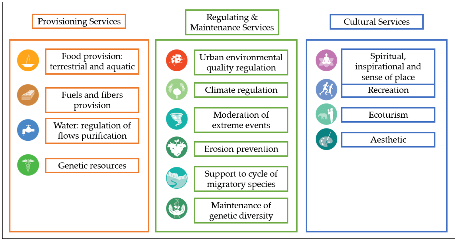
Ecosystem services support human life every day and contribute to human well-being in many ways, which are hard to define in a single notion. Hence, the Millennium Ecosystem Assessment [9] and the Common International Classification of Ecosystem Services [10] differentiate between the following ecosystem services: (a) Provisioning services (such as the supply of food via fishery production, fuel, wood, energy resources, and natural products); (b) Regulating and maintenance services (such as shoreline protection, nutrient regulation, carbon sequestration, detoxification of polluted waters, and waste disposal); and (c) Cultural services (such as tourism and recreation).

Ecosystems have great importance across many dimensions (ecological, socio-cultural, and economic) [5]. Thus, expressing the value of ecosystem services in monetary units (i.e., ecosystem service values; ESV), can prove to be of utmost importance to help raise consciousness and convey the (relative) importance of ecosystems and biodiversity to decision-makers. Indeed, monetized valuation pushes for more efficient use of limited resources and helps to select where protection and regeneration are economically more important and can be delivered at least cost [11,12]. It can also assist in determining “a fair compensation” to be paid for a loss of ES in liability regimes [5].

Historically, in the late 1990s and early 2000s, the concept of ES slowly found its way into the policy arena, e.g., through the “Ecosystem Approach” and the Global Biodiversity Assessment. In 2005, the concept of ES gained wider interest after the publication of the Millennium Ecosystem Assessment by the United Nations for policymakers [4,9]. ES are also entering the consciousness of mainstream media and business, namely through the World Business Council for Sustainable Development that has actively supported and developed this concept [13]. Many projects and groups are currently working toward better understanding, modeling, valuing, and managing ES and natural capital [4].

An increasing number of papers seeking the valuation of ES have been published over the last decades. Assessments have been conducted at local [14,15,16], national [17,18,19], continental [20,21], and global [4,5,6] scales. In the same way, databases compiling data from these primary valuation studies were created to aggregate information and facilitate public debate and policy action. Some examples of such databases include the Economic Valuation Reference Inventory [22], and the Ecosystem Service Valuation Database (ESVD; [23]).

Since the early 1990s, several researchers have investigated the applicability and the precision of benefit transfer. However, these past studies were primarily concerned with traditional methods of benefit transfer (in particular value transfer), replacing values directly from the study site to the policy site without amendments [24]. However, in the late 1990s meta-analysis started to be used, with multivariate regression being investigated for use in benefit transfer [25].

The meta-analysis (MA) is a technique that uses statistical models (meta-regressions) to summarize and evaluate previous research results. In benefit transfer, meta-regression results may be used qualitatively, to corroborate new primary results, or to transfer estimated values [26]. Meta-regression in benefit transfer summarizes the weight of the evidence and characterizes the degree of uncertainty about quality-adjusted ecosystem values. In meta-regression, the value estimates from primary valuation studies are thereby treated as individual observations [27]. Meta-regression also extends the range of primary valuation studies by allowing the estimation of values for services and functions that are constant within each primary valuation study but vary across different valuation studies [28].

Meta-analyses have been performed for specific ecosystem services, biomes, and locations. For example, Van Houtven et al. [15] assessed the cultural value of surface water quality in the United States, using 131 willingness-to-pay (WTP) estimates from 18 studies. Similarly, Hjerpe et al. [29] synthesized 127 WTP estimates from 22 different studies that provided estimations for preservation, forest restoration, and freshwater restoration also in the United States. Ghermandi et al. [30] performed a meta-analysis to determine the values of goods and services provided by wetland ecosystems, using 418 value observations derived from 170 valuation studies and 186 wetland sites worldwide. Finally, Hynes et al. [31] performed a marine recreational meta-analysis estimation, using 311 distinct value observations from 96 primary valuation studies. Nevertheless, there are no studies with a broader analysis, that estimate global meta-regression functions for Provisioning, Regulating and maintenance and Cultural ecosystem services across biomes and continents. In addition, testing the reliability of estimated meta-regression functions is relatively rare, (e.g., [32,33]). One of the main challenges is developing equations for ES that capture the local/regional characteristics of the biome and provide reliable value estimates.

Hence, the objective of this study is to estimate meta-regression functions for 3 different types of ecosystem services able to determine the ecosystem service value for 12 different types of biomes, with the possibility of these estimates being applied at the global scale. In this study, we provide the results of a meta-analysis based on the primary value estimates from the Ecosystem Service Valuation Database [23] for 3 ecosystem services (Provisioning; Regulating and maintenance; Cultural), provided by 12 main land covers (Coastal systems; Coastal wetlands; Coral reefs; Cultivated areas; Desert; Fresh water; Grasslands; Inland wetlands; Open Ocean; Temperate/Boreal forests; Tropical forests; Woodlands). In addition, complementary explanatory variables from the World Bank Data [34] and FAOSTAT [35] were gathered. Based on this review and meta-analysis, we aim to provide recommendations for future research that may enhance the use of ecosystem service valuation for policy analysis.

The remainder of this paper is structured as follows. The “Materials and Methods” section details the MA application and use in ES studies, the theoretical specification and validation method and, finally, the ESVD database and other variables used to build the models. In turn, in the “Results” section, we expose and analyze the functional forms of the models for the three ecosystem services, present the application of the models, and discusses the results. Finally, in the “Conclusions and recommendations” section, concluding remarks and observations are presented.

2. Materials and Methods

2.1. Literature on Meta-Analysis

Benefit transfer (BT) is an economic valuation tool, with the goal to adapt value estimates from past research to assess the value of a similar, but separate, change in a different resource [36]. Technically, BT uses valuation estimates from other areas (study sites) and applies them to a similar location (policy site) [3]. It is a technique that relies on primary studies and, therefore, allows for the reduction of field research constraints, both in terms of time and infrastructure. However, it can lead to over/underestimated values while the accuracy of an ESV estimate is determined by the quality of the reference studies used. Thus, peer-reviewed empirical studies from similar biophysical and socioeconomic contexts are preferred over any other type of data source [32].

BT is useful when the estimation of the economic service value cannot be obtained due to time and/or budget constraints and to, therefore, make the best possible use of the existing literature in order to evaluate the economic importance of a natural area [19]. This is possible by adopting and applying estimates from existing studies that best suit the new context, using one or more of the following BT methods: (i) benefit estimate or value transfer, which is the extrapolation of estimates from one site to another (i.e., values are directly transposed from the study site to the policy site without amendments), (ii) benefit function transfer, which is the transfer of economic functions between the sites (i.e., coefficients are used to determine the policy site values), (iii) meta-analysis, which combines the findings of independent studies related to the research topic as to summarize the body of evidence relating to a particular issue, and (iv) preference calibration, which uses existing benefit estimates derived from different methodologies and combines them to develop a theoretically consistent estimate for policy site values [37].

The meta-analysis (MA) technique can help reduce deviations in value estimates [26]. This technique was first put forward as a research synthesis method and has since been developed and applied in many fields of research, other than the area of environmental economics [38,39]. It is widely recognized that the large and increasing literature on economic valuation of ES and environmental impacts has become difficult to interpret and that there is a need for research synthesis, especially in statistical MA, to aggregate information and insights [27,40,41].

MA is by definition a quantitative analysis of statistical summary indicators reported in a series of similar empirical studies. It is a commonly used method for compiling and analyzing the data from studies towards the creation of a value function. The method synthesizes the results of multiple studies that examine the same phenomenon, through the identification of a common effect, which is then “explained” using regression techniques in a meta-regression model [40]. In the realm of environmental resource valuation, MA is commonly used in benefit transfer endeavors due to its usefulness in incorporating a structural utility framework with less strictly economic information [27,42].

2.2. Specification of the Meta-Regression

Based on consumer rationality and reasonableness, the microeconomic consumer theory is explained by two different approaches: the indifference curve approach and the utility function approach [43]. Indifference curves represent all combinations of goods and services that provide the same level of satisfaction to an individual (i.e., the same level of global utility). Implicit in an indifference curve is the marginal rate of substitution, which expresses the maximum amount of a good that one is willing to give up in exchange for one additional unit of another good, at the same level of satisfaction [43]. Utility functions represent the degree of profitability or satisfaction that we get from using goods and services, related to a measure of satisfaction relative to an economic agent. The analysis of its variation allows for explaining the behavior that results from the decisions taken by each agent to increase his/her satisfaction.

Any meta-analytic benefit transfer (MA-BT) must be based on the ecosystem service valuation theory and the utility functions theory (see Equation (1)), specific to microeconomics [42]. The general form of an MA-BT underlying the utility function is given by [24]:

$$U_i=f\left(P_i, Y_i, Q_i,Q{l}_i,Su{b}_i, H_i,I_i\right)$$

(1)

where $U_i$ is the utility (satisfaction) obtained by individual i, $P_i$ is the general price level faced by individual i, $Y_i$ is the individual revenue, $Q_i$ is the quantity of ES available to individual i, $Q{l}_i$ is the global quality of ES available to individual i, $Su{b}_i$ represents the substitutes for Q available to individual i, $H_i$ refers to other non-income attributes of individual i, and $I_i$ is the information available to individual i.

Resorting to this microeconomic theoretic, we organize the MA-BT utility theory into three axes: the “strong structural utility theoretic (SSUT) approach”, the “weak structural utility theoretic (WSUT) approach” and the “non-structural utility theoretic (NSUT) approach” (of which they only endorse the first two) [42].

Following the microeconomics reasoning, we assume that MA-BT is based on the utility function (see Equation (2)) and opt for analyzing the WSUT. Under the WSUT, each individual may choose between two alternative environmental options—ceteris paribus, a damaged ecosystem ($Q_0$) and a restored ecosystem ($Q_1$), which will assure an equilibrium situation (the maximum utility) [7,42], represented by:

$$U_{i }\left(P_i, Y_i, Q_0\right)=U_{i }\left(P_i, Y_i,-ESV, Q_1\right)$$

(2)

where $U_i$ is the utility obtained by individual i, $P_i$ is general price level faced by individual i, $Y_i$ is individual revenue, $Q_0$ quality/quantity of ES available to individual i in the absence of any payment, ESV is ecosystem service value paid by individual i, and $Q_1$ is the quality/quantity of ecosystem available to individual i after having paid for these ES.

Microeconomics utility theory will hold if both sides of this parity are equal. That is, an individual will stay at the same indifference curve if he/she gets the same level of satisfaction by consuming $Q_0$ with no payment or by consuming $Q_1$ and paying ESV in exchange. That is, the ESV the individual is willing to give up must be counterbalanced by an increase in Q. Thus, $Q_1$ > $Q_0$ after the amount has been spent.

In this study, we adopt the WSUT approach, where variables are added in the bid-function (assumed to be derived from some unidentified utility function), but keeping the flexibility to incorporate other explanatory variables into the ESV model, such as study-site characteristics, local price levels or local individual income [7]. This is the approach used in most previous MA-BT studies [7,31,44]. Our general theoretical model will focus on estimating the ESV (see Equation (3)), as a function of various explanatory variables according to the general form of the underlying conditional indirect utility function:

$$ESV=f\left(B_l,S{Q}_l,C,Q{Q}_r, I_r,P_r\right)$$

(3)

where, $B_l$ is the biome and $S{Q}_l$ the quality status for the location under analysis (l), $C$ is the continent where the study area is located, and $Q{Q}_r$ is the quality/quantity of protected areas, $I_r$ is the income and $P_r$ is the population density in the region (r) where the study area is located.

The meta-modeling approach has several advantages for BT as compared to other methods (such as value transfer or function transfer). Different from those, which are based on single studies, MA resorts to information from a collection of studies and, thus, provides more rigorous measures of central tendencies that are sensitive to the distributions of underlying study values [24].

2.3. Validity and Reliability of a Meta-Analytic Benefit Transfer

The validity and reliability of the MA-BT can be assessed by applying the concept of transfer error ($TE$), defined as [32]:

$$TE=\frac{\left|ES{V}_P-ES{V}_B\right|}{ES{V}_B}$$

(4)

where $ES{V}_P$ is the predicted value from the study site (s) and $ES{V}_B$ is the base value (“benchmark”) at the policy site. The $TE$ is often used as a validity measure of the acceptability of meta-models. Traditionally, validity requires that the values, or the value functions generated from the study site, be statistically identical to those estimated at the policy site [8]. The main objective is to find a target value of TE = 0, confirming that the estimated values from the MA-BT values are similar to those arising from the database.

There is no agreement on maximum TE levels for BT being reliable for different policy applications. The TE analysis is not supposed to judge which levels should be considered acceptable, or even conduct traditional statistical tests of BT validity. Instead, it remains a measure of reliability, especially if TE estimates are compared across meta-model specifications and restrictions, and between alternative ways of conducting BT based on the same data [7].

Therefore, we perform the following comparisons between the estimates from the meta-model and the original observations from the database:

(a)

“Value transfer” compares each ESV estimate in the database with the corresponding global mean ESV;

(b)

“Global meta function transfer” compares each ESV estimate in the database with the estimates produced by the meta-model, using mean global values for the explanatory variables;

(c)

“Local meta function transfer” compares each ESV estimate in the database with the estimates produced by the meta-model, using mean national values for the explanatory variables.

2.4. Background and Data

MA in environmental valuation is, generally, based on brief statistics and analytical conclusions taking a group of studies as data. Therefore, MA estimates can reduce the time spent to acquire data—both in the case of older studies and unpublished work (where data may not be available) and current studies (where authors may be slow to disclose data). However, even within the same methodology, combining primary data is not always possible due to conflicting data structures and different estimation procedures [42]. This might limit the MA studies’ representativeness.

A solution to this problem is the use of specialized ESV databases, which offer a wide range of detailed information about the studies taken into account, beyond the results found in the assessment. These databases give information on other factors crucial for the delimitation of a MA model, such as: the year of the study, protection status, location, type of environment, and method. In this analysis, we use the Ecosystem Service Valuation Database (ESVD, [23]), one of the biggest databases containing real values for a range of ES and biomes where the value estimates are systematized in monetary units (€/ha/year).

The ESVD was built to process and analyze the monetary estimates of ES values from different biomes in a way that is easily used by various end-users, worldwide. Composed by 267 studies and 1310 value estimates, the ESVD links various types of information from different studies with the value estimates and case study sites. These value estimates are organized by biome, ecosystem service, and country. The main biomes are “Coastal System” (CSys), “Coastal Wetland” (CWet), “Coral Reef” (CoRf), “Cultivated Area” (CuAr), “Desert” (Dser), “Grasslands” (Gras), “Inland Wetland” (InWt), “Marine” (Mari), “Temperate or Boreal forests” (TeFo), “Tropical forests” (TrFo), “Fresh water” (FrWa) and “Woodland” (Wood). The ecosystem services are Provisioning; Regulating & maintenance and; Cultural services, divided into 14 types of services (see in Figure 1). Finally, a total of 80 countries are included, 217 values from Africa; 352 values from Asia, 208 values from Europe, 180 values from Latin America and the Caribbean; 122 values from North America, 116 from Oceania, and 114 from the whole world.

Initial criteria for selecting studies from the general ESVD database were: (1) original nature of the case study data (i.e., not based on value transfer or total ecosystem value); (2) the provision of a complete set of information, including the study site location, surface area and the scale of the study (i.e., not based on a “world” scale location); (3) clear characterization of valuation methodologies used (i.e., not unknown valuation methods); (4) clear mentioning of the surface area for which the ecosystem service valuation study is applied (so that estimates of monetary values per hectare can be obtained); and (5) ES or sub-service monetary value directly linked to a specific biome/ecosystem and unit (i.e., not per person or household). Besides information on the location of each case study, the ESVD includes information on protection status and the size of the research area, enabling for the verification of whether more estimates about the same case study location are available from other sources or publications. Together with supplementary variables, coming from complementary socio-economic databases that are added to ESVD, these variables allow for further socio-economic interpretation of the monetary output values.

In order to relate an estimate of an ecosystem service to the socio-economic context of a case study site, two additional variables were included in the country table—namely the Gross national income (GNI) per capita (based on purchasing power parity in current international prices) and the average Population density (PDen; people per square kilometer). This information was obtained from the World Bank Data, which provides world development indicators by country [34]. Collected values were obtained for the years in which the studies were carried out.

Regarding protection status, many of the data points in the ESVD pertain to case studies in protected areas. This information allows the assessment of the influence of the protection status on ES value, testing whether protection excludes the user’s access to the site and consequently to the services generated or, alternatively, whether it allows for ecosystem conservation and subsequent appreciation of the services. Protection status is classified into 3 categories: Fully protected (FProt), Partially protected (PProt) or Not protected (NProt). Other complementary variables collected from the World Bank Data, used to verify the study-site protection status, were: Terrestrial Protected Areas (TProt; the percentage of protected land by country) and Marine Protected Areas (MProt; the percentage of protected territorial waters). From the Food and Agriculture Organization (FAO) statistical database [35], information on the land use characteristics was collected. Namely, the percentage of forest area (FPer) and the percentage of agricultural land (APer), which helped to understand land use and occupation characteristics with emphasis on agricultural activities and state of preservation/conservation of nature.

For each biome in the ESVD, 14 ecosystem services were identified and classified into the 3 main classes: Provisioning, Regulating and maintenance, and Cultural services (see Figure 1). This classification constitutes an important step in the linkage between ES and human well-being and will be used as a basis to perform MA-BT for ecosystem valuation. Provisioning services (ESV_Prov) are mainly composed of food provision, water provision (including regulation of water flows and water purification), fuels and fibers provision, and genetic resources provision [45]. This is an ES highly valued by humans, because of the direct impact on our day-to-day life. Regulating and maintenance services (ESV_Reg&Main) help maintaining air, climate, and water quality, moderating extreme events, maintaining soil quality, and preventing erosion. Albeit usually invisible and taken for granted, they are important for human well-being and the conservation of plants and animals [45]. Finally, cultural services (ESV_Cult) entail non-material benefits that people obtain from an ecosystem, such as aesthetic inspiration, recreation, and tourism as well as spiritual experience related to a natural environment [45].

All monetary values in the ESVD values are converted into a common reference unit, specifically 2015 ‘International’ €/ha/year, using the Purchasing Power Parity (PPP) units expressed in Euros [34,45].

3. Results

3.1. Data Summary

Based on the above-mentioned criteria, the total number of monetary value estimates included in our sample amount to 636 observations. In this study, ES value functions are estimated for Provisioning, Regulating and maintenance, and Cultural services (see Section 3.2). The estimation of each ES value function draws on a different number of observations (see

Table 1. Number of valuation studies, by service and biome, from the ESVD included.

Service 1/Biome 2	CSys	CWet	CoRf	CuAr	Dser	FrWa	Gras	InWt	Mari	TeFo	TrFo	Wood	Total
ESVProv	18	55	37	6	2	5	10	75	6	8	63	17	302
ESVReg&Main	6	58	26	7	-	1	9	36	4	16	51	11	225
ESVCult	7	14	42	-	-	4	2	11	4	10	14	1	109

Note: ¹ ESV_Prov = Provisioning Ecosystem Service Values; ESV_Reg&Main = Regulating and maintenance Ecosystem Service Values; ESV_Cult = Cultural Ecosystem Service Values; ² CSys = Coastal systems; CWet = Coastal wetlands; CoRf = Coral reefs; CuAr = Cultivated areas; Dser = Desert; FrWa = Fresh water; Gras = Grasslands; InWt = Inland wetlands; Mari = Marine; TeFo = Temp./Bor. forests; TrFo = Tropical forests; Wood = Woodland.

): Provisioning services (302; 47.5%), Regulating and maintenance services (225; 35.4%), and Cultural services (109; 17.1%).

Table 2. Meta-analysis variables description.

Variables	Description
APer	Agricultural land refers to the share of land area that is arable, under permanent crops, and under permanent pastures, by the percentage of land area.
FPer	Forest area with natural or planted stands of trees of at least 5 m in situ, by the percentage of land area.
MProt	Percentage of marine protected areas, from territorial waters of a country.
TProt	Percentage of terrestrial areas totally/partially protected, designated by national authorities.
GNI	Gross National Income per capita, using purchasing power parity rates.
PDen	Population density is midyear population divided by land area in square kilometers.
Dummies
CSys; CWet; CoRf; CuAr; Dser; FrWa; Gras; InWt; Mari; TeFo; TrFo; Wood	Biomes: Coastal systems; Coastal wetlands; Coral reefs; Cultivated areas; Desert; Fresh water; Grasslands; Inland wetlands; Marine; Temp./Bor. forests; Tropical forests; Woodland.
Euro; Asia; Ocea; LaAm; NoAm; Afric	Continents: Europe; Asia; Oceania; Latin America and Caribbean; North America; Africa.
FProt; PProt; NProt	Protection Status: Fully protected; Partially protected; Not protected.

lists and describes the main variables used in the MA.

Table 3. Summary statistics for meta-regression variables in ecosystem services.

Variables 1	Mean	Stand. Dev.	Min	Max
Provisioning Services
TProt	14.94	8.53	0.00	6.27
APer	42.78	18.99	6.27	80.89
PDen	124.60	143.77	1.70	1130.40
GNI	7481.06	10,021.30	430.00	44,740.00
Regulating and Maintenance Services
FPer	35.20	20.57	0.24	91.34
MProt	12.54	17.12	0.00	74.70
TProt	14.73	7.56	0.00	36.84
PDen	115.70	127.07	2.40	502.30
GNI	14,471.44	14,036.35	430.00	48,420.00
Cultural Services
MProt	15.52	17.63	0.00	74.82
PDen	105.23	116.90	2.30	478.30
GNI	16,750.05	13,484.39	840.00	48,420.00

Note: ¹ See Table 2 for variable descriptions.

provides summary statistics for each of these variables for every service, with the exception of the dummy variables.

The common variables in all models (Provisioning; Regulating and maintenance; Cultural) are Population density (PDen) and Gross national income per capita (GNI see Table 3). These variables show the largest mean, minimum, and maximum dispersion, representing the large differences in population and wealth in countries around the world. Additional variables were created to describe potentially influential study site characteristics. In the case of Provisioning services, these were: the agricultural areas (APer) and the terrestrial protected areas (TProt). The former represents the food, fuels, and fibers provisioned, and the latter represents regulation of flows and purification provided. In the case of Regulating and maintenance services, these were: the forest areas (FPer) and the terrestrial (TProt) and marine (MProt) protected areas. These variables express the quality/quantity of natural resources that directly influence their prevention, moderation, and support. In the case of Cultural services, these were the marine protected areas (MProt), which represent quality, namely related to the sea.

3.2. Meta-Regression Model Specification

We adopt a semi-log functional form specification for the ES value functions, which implies that the marginal effect of a change in ESV depends on income and population density [15].

The Provisioning ES value function is determined by the type of biome (D_Biome), location of the continent (D_Continent), terrestrial protected area (TProt) [46], percentage of agricultural land (APer) [47], population density (PDen) [5] and income (GNI) [15], and given by:

$$\ln \left(ES{V}_{Prov}\right)={\alpha }_0+{\alpha }_1 \ast D_{Biome}+{\alpha }_2 \ast D_{Continet}+{\alpha }_3 \ast TProt+{\alpha }_4\ast APer+{\alpha }_{5 }\ast \ln \left(PDen\right)+{\alpha }_6\times \ln \left(GNI\right)$$

(5)

where α₀ is a constant, α₁ and α₂ are dummy regression estimates, and α₃ to α₆ are variable regression estimates.

The Regulating and maintenance ES value function is determined by the type of biome (D_biome), location of the continent (D_Continent), level of protection in study area (FProt) [15], the terrestrial (TProt) and marine (MProt) protected area [46], percentage of forest land (FPer) [47], population density (PDen) [5] and income (GNI) [15], and given by:

$$\ln \left(ES{V}_{Reg\&Main}\right)={\beta }_0+{\beta }_1 \ast D_{Biome}+{\beta }_2 \ast D_{Continet}+{\beta }_3 \ast FProt+{\beta }_4 \ast FPer+{\beta }_5 \ast MProt+{\beta }_6 \ast TProt+{\beta }_7 \ast \ln \left(PDen\right)+{\beta }_8 \ast \ln \left(GNI\right)$$

(6)

where β₀ is a constant, β₁ and β₂ are dummy regression estimates, and β₃ to β₈ are variable regression estimates.

Finally, the Cultural ES value function is determined by the type of biome (D_biome), location of the continent (D_Continent), level of protection in study area (PProt) [15], marine protected area (MProt) [46], population density (PDen) [5] and income (GNI) [15], and given by:

$$\ln \left(ES{V}_{Cult}\right)={\gamma }_0+{\gamma }_1 \ast D_{Biome}+{\gamma }_2 \ast D_{Continet}+{\gamma }_3 \ast \mathrm{PProt}+{\gamma }_4 \ast MProt+{\gamma }_5 \ast \ln \left(PDen\right)+{\gamma }_6 \ast \ln \left(GNI\right)$$

(7)

where $\gamma$₀ is a constant, $\gamma$₁ and $\gamma$₂ are dummy regression estimates, and $\gamma$₃ to $\gamma$₆ are variable regression estimates.

3.3. Meta-Regression Model Results

Table 4. Meta-regression results for Provisioning (ESV_Prov), Regulating and maintenance (ESV_Reg&Main) and Cultural (ESV_Cult) ecosystem service values.

Explanatory Variables 1	Model Specification
	Provisioning Serv. Model				Regu. and Main. Serv. Model				Cultural Serv. Model
	Full		Restricted		Full		Restricted		Full		Restricted
	Coef	t-Test (sig)	Coef	t-Test (sig)	Coef	t-Test (sig)	Coef	t-Test (sig)	Coef	t-Test (sig)	Coef	t-Test (sig)
CONSTANT	−3.80	0.36	−6.41	0.01	−7.97	0.03	−3.46	0.19	−12.37	0.07	−7.37	0.03
CSy	1.93	0.19	2.68	0.01	5.10	0.01	3.98	0.01	2.09	0.40	-	-
CWet	1.51	0.24	2.22	0.01	5.31	0.01	4.19	0.01	4.70	0.05	1.35	0.20
CoRf	−0.85	0.53	-	-	5.28	0.01	4.68	0.01	5.83	0.01	2.48	0.01
CuAr	3.07	0.11	3.69	0.01	4.28	0.01	3.07	0.01
Dser	1.24	0.66	-	-
FrWa	1.41	0.49	2.17	0.19	2.79	0.28	-	-	708	0.00	-	-
Gras2	-	-	-	-	-	-	-	-	-	-	-	-
InWt	1.29	0.31	2.03	0.01	5.53	0.01	4.77	0.01	5.04	0.04	1.48	0.20
Mari	1.08	0.57	2.18	0.15	2.07	0.17	-	-	1.44	0.58	−2.47	0.12
TeFo	−1.46	0.42	-	-	4.80	0.01	3.35	0.01	0.81	0.75	−3.09	0.01
TrFo	1.37	0.29	2.06	0.01	3.47	0.01	2.40	0.01	4.80	0.04	1.20	0.20
Wood	−0.33	0.83	-	-	1.69	0.12	-	-	6.28	0.08	-	-
FProt	−0.18	0.80	-	-	−1.83	0.01	−1.73	0.01	−0.42	0.75	-	-
PProt	−0.25	0.66	-	-	−0.24	0.63	-	-	0.78	0.53	1.17	0.05
NProt2	-	-	-	-	-	-	-	-	-	-	-	-
Euro2	-	-	-	-	-	-	-	-	-	-	-	-
Asia	−1.05	0.44	-	-	0.43	0.59	-	-	−1.09	0.49	−1.75	0.06
Ocea	−0.77	0.60	-	-	1.53	0.13	-	-	−0.81	0.59	−1.33	0.16
LaAm	0.82	0.55	1.76	0.01	1.14	0.23	-	-	2.55	0.17	1.33	0.18
NoAm	−0.97	0.53	-	-	0.66	0.41	-	-	0.98	0.46	-	-
Afric	−1.20	0.45	-	-	−0.79	0.49	−2.12	0.01	0.66	0.74	-	-
APer	−0.04	0.02	−0.04	0.01	-	-	-	-	-	-	-	-
FPer	-	-	-	-	−0.01	0.24	−0.02	0.05	-	-	-	-
Mprot	−0.02	0.33	-	-	−0.02	0.25	−0.02	0.19	−0.06	0.01	−0.05	0.01
TProt	−0.05	0.14	−0.05	0.10	−0.04	0.15	−0.05	0.06	−0.03	0.40	-	-
ln_GNI	0.81	0.01	0.87	0.01	0.65	0.02	0.49	0.03	1.21	0.02	1.04	0.01
ln_PDen	0.54	0.03	0.59	0.01	0.91	0.01	0.66	0.01	0.53	0.12	0.48	0.09
N	302				225				109
R²	0.20		0.19		0.47		0.46		0.48		0.38
p-Value in ANOVA 3	0.01		0.01		0.01		0.01		0.01		0.01

Notes: Dependent variable is ln_ESV_i. ¹ See Table 2 for variable descriptions; ² Variable used as the basis for analysis of the dummies; ³ F-test of joint restriction that coefficients of excluded variables are equal to zero.

reports regression results for two model specifications; the “Full” model in which all variables are included and the “Restricted” model in which non-significant explanatory variables were excluded in a stepwise procedure (applying a cut-off significance level of 20% for the t-test). The following base values for the dummies are considered: Grasslands (Gras) for biomes; Not protected (NProt) for protection status; and Europe (Euro) for continents.

The main explanatory variables presented in all “Restricted” models were Population density (ln_PDen) and Gross national income (ln_GNI), with positive coefficient values and high significance (t-test < 0.09), which implies that an increase in population or income results in an increase ESV. As we adopt the logarithmic form for these variables, the marginal increase in ESV is decreasing in population or income.

We adopted additional explanatory variables for environmental quality, being MProt and TProt the percentage of, respectively, terrestrial and marine protected areas. Specifically, for the Provisioning model the APer (percentage of agricultural land) and for the Regulating & maintenance model the FPer (percentage of forest land) were used.

The Provisioning ES model provides a reasonable fit to the data, although it is the model with the smallest R² (0.19) and with the statistics of 0.01 in ANOVA for the restricted model. The signs of the explanatory variables are, as expected, positive for D_biome, LaAm, ln_PDen, and ln_GNI, and negative for TProt. This confirms that the other land covers analyzed tend to have a higher value than Grasslands (used as a base for the dummy biomes) and that areas located in Latin America generate larger provisioning ecosystem service values, while the ecosystem service value decreases with an increase in the percentage of protected terrestrial area. The variable APer is an exception (Coef = −0.04 and t-test < 0.01), presenting a negative coefficient, for which a positive sign was expected—which could be explained by the fact that countries with larger agricultural areas present a greater supply of provisioning services, though lower productivity levels. Significant explanatory variables present t-test < 0.19, the remaining variables were dropped. Evaluating the dummy variables for biomes, the one that presented the highest coefficient for the ESV_Prov was CuAr (Coef = 3.69 and t-test < 0.01), indicating that Cultivated areas is the key variable explaining provisioning service values.

The Regulating and maintenance ES model provides a good fit to the data, being the model with the highest R² (0.46) and with the statistics of 0.01 in ANOVA for the restricted model. The sign of the explanatory variables is as expected positive for D_biome, ln_PDen, and ln_GNI, and negative for AFric. This confirms that, as mentioned before, the other land covers analyzed tend to have a higher value than Grasslands and that areas located in Africa tend to have a lower value for this type of service (due to the lower aggregate income). The variables related to nature protection: FProt (Coef = −1.73 and t-test < 0.01), FPer (Coef = −0.02 and t-test < 0.05), MProt (Coef = −0.02 and t-test < 0.19) and TProt (Coef = −0.05 and t-test < 0.05), present negative coefficients, for which a positive sign was expected, revealing the theory that protected areas, which generally have low population density or are even inaccessible to the population, represent a low monetary value (i.e., people do not fully perceive the value of this service being generated). Significant explanatory variables present t-test < 0.19, the remaining variables were dropped. In the ESV_Reg&Main the largest coefficient for biome was observed in InWt (Coef = 4.77 and t-test < 0.01), although many others such as CoRf, CWet, and CSys, (Coef = 4.68; 4.19; 3.98 and t-test < 0.01, respectively) also presented high values, these biomes hold a series of important services, such as climate moderation, erosion prevention, maintenance, and support for different species.

The Cultural ES model also presents a good fit to the data, with an R² (0.38) and with the statistics of 0.01 in ANOVA for the restricted model. The sign of the explanatory variables is as expected positive for PProt, ln_PDen, and ln_GNI, LaAm and negative for MProt, Asia, Ocea. This explains that partially protected areas make it possible for people to access and benefit from the services generated. Moreover, Latin America is the area that presents the largest Cultural ES (primary studies mainly from the Caribbean coast). The D_biome variables Mari (Coef = −2.47 and t-test < 0.12) and TeFo (Coef = −3.09 and t-test < 0.01), present negative coefficients, for which a positive sign was expected, due to the small number of studies related to cultural services involving these land covers in the ESVD. In the ESV_Cult the largest coefficient was CoRf (Coef = 2.48 and t-test < 0.01), explaining the high value of services associated with the Coral reefs biome, which provides services such as ecotourism, recreation, and aesthetics, receiving thousands of tourists annually.

The model with the least good fit was the Provisioning ES model (R² = 0.19), followed by the Cultural ES model with a reasonable fit (R² = 0.38) and the Regulating and maintenance ES model” with a reasonably good fit (R² = 0.46) for the restricted models. Although these values are low as compared to other ESV meta-analysis studies (see

Table 5. Studies applying the meta-analysis for ESV.

Authors	Location	Ecosystem Service	Biome	R²	Samp. Size	Cut-Off in t-Test 1
Rosenberger & Loomis [24]	United States and Canada	Outdoor activities	-	0.26	682	0.20
Bateman & Jones [41]	British Forest—Great Britain	Recreation	Woodlands	0.71	77	0.38
Van Houtven et al. [15]	United States	Water quality	-	0.59–0.61	131	0.10
Lindhjem & Navrud [7]	Norway, Sweden, and Finland	Non-use values related to biodiversity	Forests	0.81–0.87	72	0.20
Ghermandi et al. [30]	World	Flood protection, water quality, and water storage and supply	Wetlands	0.49–0.46	416	0.10
Hjerpe et al. [29]	United States	Forest and freshwater restoration	Forests and Fresh waters	0.58–0.60	127	0.18
Rao et al. [44]	World coastal area	Shoreline protection	Coastal Areas	0.44–0.45	90	0.10
Hynes et al. [31]	World	Recreation services	Coastal Areas	0.25–0.65	311	0.10

Note: ¹ Values presented for the final/best model presented.

), a great variability is observed in these studies, with R² between 0.25 and 0.87. The explanation for these values is related to the large number of observed studies that presented different characteristics like the location, valuation method, and different years in which the study was performed. For example, [24,30,31] presented large samples, with 682, 416, and 311 observations, respectively. In addition, these studies were applied in wide areas, covering several countries.

As previously exposed, the cut-off for the significance level adopted in the t-student test for the model variables was 20%, which eventually diminished the reliability of the models (i.e., it is common to use “cut-off points” of 0.5%, 1%, 5% or even 10%). Nevertheless, authors such as [7,24,29,41] used t-values similar to those adopted in our research. It will be demonstrated, in the next section, that the transfer errors obtained using these value functions are smaller than those obtained using other benefit transfer techniques.

3.4. Value Function Transfer Errors and Estimates

The validity of environmental benefit transfer has been the subject of a number of studies [7,48,49]. In all of them, the validity has been tested by stating a null hypothesis of no difference between the original study result and the benefit transfer estimate [50]. As in those studies, in this study we seek to verify the differences between the estimated values from MA-BT with the values from the ESVD database, using the Transfer Error technique (see Section 2.3).

3.4.1. Transfer Errors

To assess the accuracy of the estimated ES value meta-models, in order to justify their adoption in future research covering different locations with varied characteristics, we determined the transfer errors associated with Value transfer, Global meta function transfer, and Local meta function transfer (see Section 2.3). This is done for the Provisioning, Regulating and maintenance, and Cultural ES value functions (see

Table 6. Comparison of values and transfer errors (TE) per biome for Provisioning ES, based on Value transfer, Global meta function transfer, and Local meta function transfer (in 2015 €/ha/yr).

	Value Transfer		Global Meta Function Transfer		Local Meta Function Transfer
Biome 1	Value	TE (ETE1)	Value	TE (ETE2)	Value	TE (ETE3)
CSys	1336.0	926.2	81.9	56.7	185.7	11.4
CWet	362.7	1228.2	30.7	103.9	66.0	10.1
CoRf	1463.7	7.0 × 106	10.3	5.0 × 104	23.1	1.6 × 104
CuAr	2795.2	4.2 × 105	141.7	2.2 × 104	741.8	1.4 × 104
Dser	82.5	106.2	1.5	2.0	1.5	2.0
FrWa	594.9	107.3	59.7	10.7	120.5	15.6
Gras	164.9	4.5 × 104	2.8	769.9	8.1	106.3
InWt	176.8	2013.6	6.2	71.0	15.8	54.7
Mari	50.8	2.76	27.6	1.4	48.0	4.0
TeFo	68.1	203.2	10.8	32.1	14.3	41.0
TrFo	277.3	297.8	31.2	33.3	58.3	19.6
Wood	110.6	1.1 × 106	4.6	2.7 × 106	15.4	6.5 × 106

Note: ¹ CSys = Coastal systems; CWet = Coastal wetlands; CoRf = Coral reefs; CuAr = Cultivated areas; Dser = Desert; FrWa = Fresh water; Gras = Grasslands; InWt = Inland wetlands; Mari = Marine; TeFo = Temp./Bor. forests; TrFo = Tropical forests; Wood = Woodland.

,

Table 7. Comparison of values and transfer errors (TE) per biome for Regulating and maintenance ES, based on Value transfer, Global meta function transfer, and Local meta function transfer (in 2015 €/ha/yr).

	Value Transfer		Global Meta Function Transfer		Local Meta Function Transfer
Biome 1	Value	TE (ETE1)	Value	TE (ETE2)	Value	TE (ETE3)
CSys	941.9	7.6	258.3	1.8	1381.8	3.8
CWet	5088.3	267.3	430.6	22.5	943.2	12.3
CoRf	7074.0	3189.4	383.9	173.0	1236.6	18.6
CuAr	425.6	20.0	134.4	6.2	215.0	1.7
Dser	-	-	-	-	-	-
FrWa	115.5	0.0	29.8	0.7	29.8	0.7
Gras	111.9	1464.9	11.7	153.3	22.2	37.2
InWt	1660.2	1430.5	188.8	162.6	747.4	17.6
Mari	748.3	260.8	18.0	6.2	28.7	1.4
TeFo	641.8	44.9	94.7	6.4	197.2	5.4
TrFo	135.7	111.0	16.4	13.1	48.4	9.6
Wood	199.0	117.5	17.9	10.7	41.4	25.0

Note: ¹ See Table 6 for variable descriptions.

and

Table 8. Comparison of values and transfer errors (TE) per biome for Cultural ES, based on Value transfer, Global meta function transfer, and Local meta function transfer (in 2015 €/ha/yr).

	Value Transfer		Global Meta Function Transfer		Local Meta Function Transfer
Biome 1	Value	TE (ETE1)	Value	TE (ETE2)	Value	TE (ETE3)
CSys	156.9	156.3	90.6	90.0	186.9	33.7
CWet	3099.8	119.3	152.6	5.6	267.0	5.1
CoRf	5340.9	2138.0	308.9	123.6	1695.3	17.1
CuAr	-	-	-	-	-	-
Dser	-	-	-	-	-	-
FrWa	651.4	0.5	16.1	1.0	36.2	0.9
Gras	1.4	0.2	48.6	35.3	58.2	46.4
InWt	681.5	15.3	142.4	3.0	234.0	3.3
Mari	311.8	316.9	7.4	7.2	20.6	1.6
TeFo	878.8	1.9 × 104	9.1	204.8	13.2	180.5
TrFo	275.4	38.3	38.0	5.1	85.6	6.2
Wood	3840.5	0.0	196.7	0.9	196.7	0.9

Note: ¹ See Table 6 for variable descriptions.

, respectively).

The ecosystem service values and transfer errors per biome related to the estimates for the Provisioning ES are presented in Table 6. Overall, it can be concluded that the transfer error is reduced when moving from Value transfer to Global meta function transfer and, in turn, that the transfer error is further reduced when moving to Local meta function transfer. Notable exception holds for Wood, which demonstrates the lowest transfer error when using Value transfer. This is explained by the fact that this variable was dropped from the restricted model (not significant according to the t-test). Also, in some cases, the transfer error increases slightly when moving from Global meta function transfer to Local meta function transfer (such as for FrWa, Mari, and TeFo), which is explained by the large variation of values in the ESVD database that contained studies from different countries, continents, and years, and in the case of those biomes, ranging from 1.5 to 3000.0 €/ha/year.

Table 7 presents the ecosystem service values and transfer errors per biome associated with the estimates for the Regulating and maintenance ES. According to the analysis of the previous table, the TE is reduced when moving from Value transfer to Global meta function transfer and then moving to Local meta function transfer. In this case, the exceptions hold for CSys and Wood, which demonstrate the lowest transfer error when using Global meta function transfer. This is explained by the variation of the values presented in the ESVD database for these biomes. No transfer error is observed for FrWa when using value transfer, as only one observation for this biome is available in the ESVD. Finally, no value estimate and transfer error were calculated for Dser because there are no primary value estimates data for this biome in the ESVD.

Finally, Table 8 presents the ecosystem service values and transfer errors per biome associated with the estimates for the Cultural ES. Again, it can be observed that the transfer error is reduced when moving from Value transfer to Global meta function transfer and next, to Local meta function transfer. Although there are exceptions, such as for FrWa, InWt, and TrFo, which presented similar TE across Global and Local meta function transfer. One prominent exception holds for Gras, which demonstrates the lowest transfer error when using Value transfer. This is justified because it contained only two observations for this biome in the database. No transfer error is observed for Wood when using value transfer, as only one observation for this biome is available in the ESVD. Finally, no value estimates and transfer errors were calculated for CuAr and Dser because there are no primary value estimates for these biomes in the ESVD.

Hence, it can be concluded that transfer errors are reduced significantly when using Global meta function transfer and, in particular, Local meta function transfer as compared to Value transfer. This is justified because value function transfers allow the analyst greater control over differences across sites, they can yield lower transfer errors than simple mean value transfers [51]. In fact, by comparison, value functions offer a greater reflection of the variability of a sample, because the study is dealing with a database with great variability. For this reason, finding a model that, for the most part, has obtained a superior result than other benefit transfers techniques, is an advance that justifies its application given the heterogeneity of the data.

Value functions should thereby draw upon common drivers of preferences reflected in economic theory, including only those variables applicable to all sites [52]. Economic theory suggests that the benefits from environmental improvements should be determined by [53]: (i) change in provision, (ii) distance to the site, (iii) distance to substitute sites, and (iv) characteristics of the valuing individual (in particular income). That is why Local meta function transfer presents the lowest TE, for addressing these preferences and reflecting the context of each country.

3.4.2. Local Value Function Transfer Estimates

Ecosystem service value estimates per biome for Provisioning (ESV_Prov), Regulating and maintenance (ESV_Reg&Main), and Cultural (ESV_Cult) ecosystem services, are presented in

Table 9. Estimated ES values per biome for Provisioning (ESV_Prov), Regulating and maintenance (ESV_Reg&Main), and Cultural (ESV_Cult) ecosystem services, using Local meta function transfer and mean national values for the explanatory variables (in 2015 €/ha/yr).

Ecosystem Service 1	CSys	CWet	CoRf	CuAr	Dser	FrWa	Gras	InWt	Mari	TeFo	TrFo	Wood
ESVProv	44.5	28.0	3.0	122.0	3.0	26.7	3.0	23.1	27.0	3.0	23.9	3.0
ESVReg&Main	193.2	238.1	389.9	78.1	-	3.6	3.6	425.8	3.6	103.3	39.9	3.6
ESVCult	127.1	491.6	1520.7	-	-	127.1	127.1	555.3	10.8	5.8	420.8	127.1
ESVTotal	364.8	757.7	1913.6	200.1	3.0	157.4	133.7	1004.2	41.3	112.2	484.5	133.7

Note: ¹ ESV_Prov = Provisioning Ecosystem Service Values; ESV_Reg&Main = Regulating and maintenance Ecosystem Service Values; ESV_Cult = Cultural Ecosystem Service Values; ESV_Total = Total Ecosystem Service Values.

. Value estimates are thereby based on the restricted models presented in Table 4, using local value function transfer and mean values for the explanatory variables (from Table 3).

The values found in Table 9 show great variability, with values ranging from ESV_Total = 3.0 €/ha/year for Desert areas to ESV_Total = 1 913.5 €/ha/year for Coral reefs. The biomes that provide largest total economic value are Coral reefs (CoRf = 1 913.6 €/ha/year), Inland wetlands (InWt = 1 004.2 €/ha/year) and Coastal wetlands (CWet = 757.7 €/ha/year). These biomes, in addition to standing out for providing a great diversity of ecosystem services, are also the smallest biomes in terms of the area around the globe and, consequently, the scarcest and, thus, most valuable. In fact, in studies that analyzed ES globally [4,5,54], these biomes were also those with the highest value.

Provisioning services represent the lowest values and are related to the supplies of products (such as food, materials, or water) with values close to their direct use values [5]. The largest provisioning ES values are provided by Cultivated areas (CuAr = 121.9 €/ha/year) and Coastal System (CSys = 44.5 €/ha/year). The lowest values were found for Coral reefs, Desert, Grasslands, and Temp./Bor. forests (CoRf, Dser, Gras, and TeFo, with a value of 3.0 €/ha/year each).

Regulating and maintenance services are linked to more indirect benefits, which are related to quality, moderation, and prevention in environmental factors (Rao et al., 2015). The largest Regulating & maintenance ES values are provided by Inland wetlands (InWt = 425.8 €/ha/year), followed by Coral reefs (CoRf = 389.9 €/ha/year) and Coastal wetlands (CWet = 238.1 €/ha/year), demonstrating a high added value for areas in transition, notably coastal areas. The lowest values were found for the Marine and Woodland areas (Mari and Wood, with a value of 3.6 €/ha/year each).

Cultural services represent the largest values, because they involve complex issues such as aesthetics, generated inspiration, and spirituality, which can be considered incommensurable values as the perception about the environment varies from person to person [5,31]. The largest cultural ES values are provided by Coral reefs (CoRf = 1 520.7 €/ha/year), Inland wetlands (InWt = 555.3 €/ha/year) and Coastal wetlands (CSys = 491.6 €/ha/year). The lowest values were found for the Marine areas (Mari = 10.8 €/ha/year) and Temp./Bor. forests (TeFo = 5.8 €/ha/year).

It is necessary to be cautious when valuing ecosystem services since, although the aim of pricing is to use values in monetary units, they serve as a tool to provide better insight into the economic benefits of ecosystem goods and services. We do not try to find the shortcomings and limitations of monetary valuation, both in relation to ecosystem services and man-made goods and services [5,55].

When ESV’s models are created and values for biomes are estimated, this does not mean the biomes in question should be treated as private commodities that can be traded in private markets. Most of those ecosystem services are public goods or the product of common assets that cannot, or should not, be sold. Although the flowers, fruits, wood, and leaves enter the market as private goods, the ecosystems that produce them, as for example forests and woodlands, are common assets. Their values are an estimation of the benefits to society expressed in a way that communicates with a broad audience. This can help to raise awareness of the importance of ecosystem services to society and serve as a powerful and essential communication tool to inform better, more balanced decisions regarding trade-offs with policies that enhance the gross domestic product but damage ecosystem services [4].

4. Conclusions and Recommendations

Ecosystem service value (ESV) meta-models were designed to provide access to values in monetary units for ecosystem services (ES), taking into account the local context of the country and area under analysis. Through their application, it is possible to estimate values for 3 different types of ecosystem services (Provisioning; Regulating and maintenance; Cultural) and 12 different types of land covers (Coastal systems; Coastal wetlands; Coral reefs; Cultivated areas; Desert; Fresh water; Grasslands; Inland wetlands; Open ocean; Temperate/Boreal forests; Tropical forests; Woodlands) in the world. To this end, we built on the review and meta-analysis of the Ecosystem Service Valuation Database (ESVD).

The highest ES values were those associated with Cultural services, followed by Regulating and maintenance and, finally, Provisioning services. Among the biomes with greater associated ecosystem service values are Coral reefs, Inland wetlands, and Coastal wetlands that, among other characteristics, are transitional, aquatic-terrestrial biomes that are scarce and provide a great diversity of services.

It was observed that local independent variables, such as income, population, agricultural and forest area, and those related to the level of environmental protection, are significant explanatory variables and, thus, comprise the ESV meta-models. The application of the meta-functions provides values with greater accuracy as compared to simple value transfer and, as shown by the transfer error analysis, the application of local variables (local meta function transfer) further increases this precision.

A meta-analysis, thus, reduces value transfer errors by taking into account local specifications to determine ESV’s. There are several studies that have used meta-models for the valuation of specific ecosystem services and biomes (e.g., [15,29,30,31]), however, we have not found such a comprehensive study in the literature that has determined the value of 3 ecosystem services for 12 different biomes in the world. Even considering that there are certain transfer errors with the application of meta-models, as compared to other benefit transfer techniques (such as value transfer and value function transfer) the meta-analysis technique has shown to be the best way to estimate the value of ecosystem services.

Some caveats to this study remain. First, there are improvements that can be made to the results, such as updating the database, adopting other explanatory variables, or even different functional forms. Second, the adoption of the ESVD, which although very broad, has some limitations, such as the necessity for further studies for biomes such as Fresh water, which presented only one study for Regulating and maintenance ES, and Woodland, which presented only one study for Cultural ES. Moreover, biomes such as Cultivated areas, Desert, and Marine presented few valuation studies, which could directly influence their estimated ES values. Third, ecosystem services and values from marine biomes face particular challenges as these are scarcely studied and poorly understood (e.g., [56,57]). Finally, it was not possible to estimate values for urban areas, albeit they are important because they have a constant relationship with human well-being through services provided by areas such as parks, squares, and green spaces, as there were no studies analyzing this land cover in the ESVD database.

We expect this study to be a step further in studies that involve valuing ecosystem services and provide a basis for future research. Not in the least because ecosystem services and values are increasingly considered in environmental planning and nature conservation. Using reliable ecosystem service value estimates from local value functions for 3 ecosystem service types across 12 biomes will facilitate this process—in particular in data-poor circumstances.

References

- Say, J.B. Cours Complet D’économie Politique Pratique; Nabu Press: Paris, France, 1829; p. 790. [Google Scholar]
- Bordt, M.; Saner, M. Which ecosystems provide which services? A meta-analysis of nine selected ecosystem services assessments. One Ecosyst. 2019, 4, e31420. [Google Scholar] [CrossRef]
- Brouwer, R. Environmental value transfer: State of the art and future prospects. Ecol. Econ. 2000, 32, 137–152. [Google Scholar] [CrossRef]
- Costanza, R.; De Groot, R.; Sutton, P.; Van der Ploeg, S.; Anderson, S.J.; Kubiszewski, I.; Farber, S.; Turner, R.K. Changes in the global value of ecosystem services. Glob. Environ. Chang. 2014, 26, 152–158. [Google Scholar] [CrossRef]
- De Groot, R.; Brander, L.; Van Der Ploeg, S.; Costanza, R.; Bernard, F.; Braat, L.; Christie, M.; Crossman, N.; Ghermandi, A.; Hein, L.; et al. Global estimates of the value of ecosystems and their services in monetary units. Ecosyst. Serv. 2012, 1, 50–61. [Google Scholar] [CrossRef]
- Díaz, S.; Demissew, S.; Carabias, J.; Joly, C.; Lonsdale, M.; Ash, N.; Larigauderie, A.; Adhikari, J.R.; Arico, S.; Báldi, A.; et al. The IPBES Conceptual Framework—Connecting nature and people. Curr. Opin. Environ. Sustain. 2015, 14, 1–16. [Google Scholar] [CrossRef] [Green Version]
- Lindhjem, H.; Navrud, S. How reliable are meta-analyses for international benefit transfers? Ecol. Econ. 2008, 66, 425–435. [Google Scholar] [CrossRef] [Green Version]
- Navrud, S.; Ready, R. Lessons Learned for Environmental Value Transfer. In Environmental Value Transfer: Issues and Methods; Navrud, S., Ready, R., Eds.; Springer: Amsterdam, The Netherlands, 2007; pp. 283–290. [Google Scholar]
- Alcamo, J. Ecosystems and Human Well-Being: A Framework for Assessment; Island Press: Washington, DC, USA, 2003; p. 266. [Google Scholar]
- Haines-Young, R.; Potschin, M.B. The Common International Classification of Ecosystem Services. European Environment Agency. Available online: https://www.cices.eu (accessed on 16 June 2021).
- Crossman, N.D.; Bryan, B.A. Identifying cost-effective hotspots for restoring natural capital and enhancing landscape multi-functionality. Ecol. Econ. 2009, 68, 654–668. [Google Scholar] [CrossRef]
- Crossman, N.D.; Bryan, B.A.; Summers, D.M. Carbon payments and low-cost conservation. Conserv. Biol. 2011, 25, 835–845. [Google Scholar] [CrossRef]
- WBCSD. Biodiversity and Ecosystem Services: Scaling Up Business Solutions: Company Case Studies That Help Achieve Global Biodiversity Targets; WBCSD Ecosystems: Geneva, Switzerland, 2012; p. 67. [Google Scholar]
- Maynard, S.; James, D.; Davidson, A. The development of an ecosystem services framework for South East Queensland. Environ. Manag. 2010, 45, 881–895. [Google Scholar] [CrossRef]
- Van Houtven, G.; Powers, J.; Pattanayak, S.K. Valuing water quality improvements in the United States using meta-analysis: Is the glass half-full or half-empty for national policy analysis? Resour. Energy Econ. 2007, 29, 206–228. [Google Scholar] [CrossRef] [Green Version]
- Schröter, M.; Barton, D.N.; Remme, R.P.; Hein, L. Accounting for capacity and flow of ecosystem services: A conceptual model and a case study for Telemark, Norway. Ecol. Indic. 2014, 36, 539–551. [Google Scholar] [CrossRef]
- Perez-Verdin, G.; Sanjurjo-Rivera, E.; Galicia, L.; Hernandez-Diaz, J.C.; Hernandez-Trejo, V.; Marquez-Linares, M.A. Economic valuation of ecosystem services in Mexico: Current status and trends. Ecol. Serv. 2016, 21, 6–19. [Google Scholar] [CrossRef]
- Schröter, M.; Albert, C.; Marques, A.; Tobon, W.; Lavorel, S.; Maes, J.; Brown, C.; Klotz, S.; Bonn, A. National Ecosystem Assessments in Europe: A Review. BioScience 2016, 66, 813–828. [Google Scholar] [CrossRef] [Green Version]
- Alves, F.; Roebeling, P.; Pinto, P.; Batista, P. Valuing ecosystem service losses from coastal erosion using a benefits transfer approach: A case study for the Central Portuguese coast. J. Coast. Res. 2009, 56, 1169–1173. [Google Scholar]
- Paprotny, D.; Terefenko, P.; Giza, A.; Czapliński, P.; Vousdoukas, M.I. Future losses of ecosystem services due to coastal erosion in Europe. Sci. Total Environ. 2021, 760, 144310. [Google Scholar] [CrossRef]
- Roebeling, P.; Costa, L.; Magalhães-Filho, L.; Tekken, V. Ecosystem service value losses from coastal erosion in Europe: Historical trends and future projections. J. Coast. Conserv. 2013, 17, 389–395. [Google Scholar] [CrossRef]
- De Civita, P.; Filion, F.; Frehs, J. EVRI-Environmental Valuation Reference Inventory. Environment and Climate Change Canada. Available online: https://www.evri.ca (accessed on 20 December 2020).
- ESVD. Ecosystem Service Valuation Database. Foundation for Sustainable Development. Available online: https://www.es-partnership.org/esvd (accessed on 20 December 2020).
- Rosenberger, R.; Loomis, J. Using meta-analysis for benefit transfer: In-sample convergent validity tests of an outdoor recreation database. Water Res. Resour. 2000, 36, 1097–1107. [Google Scholar] [CrossRef]
- Desvousges, W.; Johnson, F.; Banzhaf, H. Environmental Policy Analysis with Limited Information: Principles and Applications of the Transfer Method; Edward Elgar: Northampton, UK, 1998; p. 244. [Google Scholar]
- Hoehn, J. Methods to address selection effects in the meta regression and transfer of ecosystem values. Ecol. Econ. 2006, 60, 389–398. [Google Scholar] [CrossRef]
- Smith, V.K.; Pattanayak, S.K. Is meta-analysis a Noah’s Ark for non-market valuation? Environ. Resour. Econ. 2002, 22, 271–296. [Google Scholar] [CrossRef]
- Johnston, R.J.; Besedin, E.Y.; Iovanna, R.; Miller, C.J.; Wardwell, R.F.; Ranson, M.H. Systematic variation in willingness to pay for aquatic resource improvements and implications for benefit transfer: A meta-analysis. Can. J. Agric. Econ./Rev. Can. D’agroeconomie 2005, 53, 221–248. [Google Scholar] [CrossRef]
- Hjerpe, E.; Hussain, A.; Phillips, S. Valuing type and scope of ecosystem conservation: A meta-analysis. J. For. Econ. 2015, 21, 32–50. [Google Scholar] [CrossRef] [Green Version]
- Ghermandi, A.; van den Bergh, J.C.J.M.; Brander, L.M.; de Groot, H.L.F.; Nunes, P.A.L.D. Values of natural and human-made wetlands: A meta-analysis. Water Res. Resour. 2010, 46, W12516. [Google Scholar] [CrossRef] [Green Version]
- Hynes, S.; Ghermandi, A.; Norton, D.; Williams, H. Marine recreational ecosystem service value estimation: A meta-analysis with cultural considerations. Ecosyst. Serv. 2018, 31, 410–419. [Google Scholar] [CrossRef]
- Ready, R.; Navrud, S. International benefit transfer: Methods and validity tests. Ecol. Econ. 2006, 2, 429–434. [Google Scholar] [CrossRef]
- Subroy, V.; Gunawardena, A.; Polyakov, M.; Pandit, R.; Pannell, D.J. The worth of wildlife: A meta-analysis of global non-market values of threatened species. Ecol. Econ. 2019, 164, 106374. [Google Scholar] [CrossRef]
- World Bank. The World Bank—Databank. World Bank Group. Available online: https://databank.worldbank.org/ (accessed on 20 June 2020).
- FAOSTAT. Food and Agriculture Data. Food and Agriculture Organization of the United Nations. Available online: http://www.fao.org/faostat/en/#data (accessed on 20 December 2020).
- Smith, V.K.; Van Houtven, G.; Pattanayak, S.K. Benefit transfer via preference calibration: ‘Prudential algebra’ for policy. Land Econ. 2002, 78, 132–152. [Google Scholar] [CrossRef]
- Bergstrom, J.C.; De Civita, P. Status of benefit transfer in the United States and Canada: A review. Can. J. Agric. Econ. 1999, 47, 79–87. [Google Scholar] [CrossRef]
- Glass, G.V. Primary, secondary and meta-analysis of research. Educ. Res. 1976, 5, 3–8. [Google Scholar] [CrossRef]
- Nelson, J.P.; Kennedy, P.E. The use (and abuse) of meta-analysis in environmental and natural resource economics: An assessment. Environ. Resour. Econ. 2009, 42, 345–377. [Google Scholar] [CrossRef]
- Stanley, T.D. Wheat from chaff: Meta-analysis as quantitative literature review. J. Econ. Pers. 2001, 15, 131–150. Available online: https://www.jstor.org/stable/2696560 (accessed on 20 December 2020). [CrossRef]
- Bateman, I.J.; Jones, A.P. Contrasting conventional with multi-level modeling approaches to meta-analysis: Expectation consistency in U.K. Woodland recreation values. Land Econ. 2003, 79, 235–258. [Google Scholar] [CrossRef]
- Bergstrom, J.C.; Taylor, L.O. Using meta-analysis for benefits transfer: Theory and practice. Ecol. Econ. 2006, 60, 351–360. [Google Scholar] [CrossRef] [Green Version]
- Pindyck, R.S.; Rubinfeld, D.L. Microeconomics, 5th ed.; Prentice Hall: São Paulo, Brazil, 2005; p. 771. [Google Scholar]
- Rao, N.; Ghermandi, A.; Portela, R.; Wang, X. Global values of coastal ecosystem services: A spatial economic analysis of shoreline protection. Ecosyst. Serv. 2015, 11, 95–105. [Google Scholar] [CrossRef]
- FAO. State of World Fisheries and Aquaculture; Sustainability in Action; FAO: Rome, Italy, 2020; p. 196. [Google Scholar]
- Agardy, M.T. Advances in marine conservation: The role of marine protected areas. Trends Ecol. Evol. 1994, 9, 267–270. [Google Scholar] [CrossRef]
- De Beurs, K.M.; Henebry, G.M. Land surface phenology, climatic variation, and institutional change: Analyzing agricultural land cover change in Kazakhstan. Remote Sens. Environ. 2004, 89, 497–509. [Google Scholar] [CrossRef]
- Brouwer, R.; Spaninks, A. The Validity of Environmental Benefit Transfer: Further Empirical Testing. Environ. Resour. Econ. 1999, 14, 95–117. [Google Scholar] [CrossRef]
- Bergland, O.; Magnussen, K.; Navrud, S. Benefit Transfer: Testing for Accuracy and Reliability. In Comparative Environmental Economic Assessment; Florax, R.J.G.M., Nijkamp, P., Willis, K., Eds.; Edward Elgar: Cheltenham, UK, 2002. [Google Scholar]
- Kristofersson, D.; Navrud, S. Validity tests of benefit transfer—Are we performing the wrong tests? Environ. Resour. Econ. 2005, 30, 279–286. [Google Scholar] [CrossRef]
- Pearce, D.W.; Whittington, D.; Georgiou, S. Project and Policy Appraisal: Integrating Economics and Environment; OECD: Paris, France, 1994; p. 346. [Google Scholar]
- Roebeling, P.; Abrantes, N.; Ribeiro, S.; Almeida, P. Estimating cultural benefits from surface water status improvements in freshwater wetland ecosystems. Sci. Total Environ. 2016, 545, 219–226. [Google Scholar] [CrossRef]
- Bateman, I.J.; Brouwer, R.; Ferrini, S.; Schaafsma, M.; Barton, D.N.; Dubgaard, A.; Hasler, B.; Hime, S.; Liekens, I.; Navrud, S.; et al. Making benefit transfers work: Deriving and testing principles for value transfers for similar and dissimilar sites using a case study of the non-market benefits of water quality improvements across Europe. Environ. Resour. Econ. 2011, 50, 365–387. [Google Scholar] [CrossRef] [Green Version]
- Costanza, R.; d’Arge, R.; De Groot, R.; Farber, S.; Grasso, M.; Hannon, B.; Limburg, K.; Naeem, S.; O’Neill, R.V.; Paruelo, J.; et al. The value of the world’s ecosystem services and natural capital. Nature 1997, 387, 253–259. [Google Scholar] [CrossRef]
- Thompson, B.H.; Paradise, R.E.; Mccarty, P.; Segerson, K.; Ascher, W.; McKenna, D.C.; Biddinger, G. Valuing the Protection of Ecological Systems and Services. A Report of the EPA Science Advisory Committee, EPA-SAB-09-012; Science Advisory Board, U.S.U.S. Environmental Protection Agency Science Advisory Board: Washington, DC, USA, 2009; p. 138.
- Townsend, M.; Davies, K.; Hanley, N.; Hewitt, J.E.; Lundquist, C.J.; Lohrer, A.M. The Challenge of Implementing the Marine Ecosystem Service Concept. Front. Mar. Sci. 2018, 5, 359. [Google Scholar] [CrossRef] [Green Version]
- Austen, M.C.; Andersen, P.; Armstrong, C.; Döring, R.; Hynes, S.; Levrel, H.; Oinonen, S.; Ressurreição, A. Valuing Marine Ecosystems: Taking into Account the Value of Ecosystem Benefits in the Blue Economy. In EMB Future Science Brief. N.5; European Marine Board: Oostende, Belgium, 2019; p. 36. [Google Scholar]
Figure 1.
Ecosystem service values division [45].