Taking Kinetic Evaluations of Degradation Data to the Next Level with Nonlinear Mixed-Effects Models

Abstract

When data on the degradation of a chemical substance have been collected in a number of environmental media (e.g., in different soils), two strategies can be followed for data evaluation. Currently, each individual dataset is evaluated separately, and representative degradation parameters are obtained by calculating averages of the kinetic parameters. However, such averages often take on unrealistic values if certain degradation parameters are ill-defined in some of the datasets. Moreover, the most appropriate degradation model is selected for each individual dataset, which is time consuming and then requires workarounds for averaging parameters from different models. Therefore, a simultaneous evaluation of all available data is desirable. If the environmental media are viewed as random samples from a population, an advanced strategy based on assumptions about the statistical distribution of the kinetic parameters across the population can be used. Here, we show the advantages of such simultaneous evaluations based on nonlinear mixed-effects models that incorporate such assumptions in the evaluation process. The advantages of this approach are demonstrated using synthetically generated data with known statistical properties and using publicly available experimental degradation data on two pesticidal active substances.

1. Introduction

For the assessment of risks caused by the release of man-made chemicals into the environment [1], a multitude of standardised experiments are carried out to characterise their environmental fate and behaviour. The degradation of chemicals is most often examined in laboratory incubation experiments using representative samples from environmental media such as soil, water and sediment. As laboratory conditions are necessarily artificial in some aspects, degradation in soil is sometimes also investigated in the field. In the case of soils, often, a number of individual experiments with different types of soil and/or at different locations are performed with the same substance.

Based on the guidance of the European Union (EU) [2,3] or North America [4,5], each set of data is then evaluated separately using nonlinear regression [6]. After normalisation to reference temperature and moisture, the individual results such as degradation rate constants, half-lives or formation fractions of transformation products are then averaged to obtain so-called modelling endpoints that serve as input in environmental exposure models. These endpoints are considered representative for the degradation in a relevant environmental compartment such as the agricultural soils in EU member states.

The variability of the results of the individual experiments is only taken into account if it can be attributed to a covariate such as soil pH. Other observed variabilities encountered in the environment are assumed to be covered by the standard scenarios used in the exposure scenarios [7,8,9,10].

Here, we show that the simultaneous evaluation of all datasets available for a certain type of media, as opposed to the separate evaluations described above, can make the endpoints more robust and can reduce the complexity of the model selection process.

When degradation is comparatively slow, i.e., only little degradation occurs within the maximum incubation time, some experiments yield degradation rate constants very close to zero with large confidence intervals. If such parameters are tested for significant difference from zero, they often fail the test. Parameters affected by this problem are often rate constants for the second, slower degradation phase in biphasic degradation models or the rate constants for slowly degrading transformation products.

Regulatory guidance for pesticide risk assessments in the EU recommends not considering such ill-determined rate constants when calculating geometric mean rate constants over the different soil types. However, ignoring such ill-determined rate constants in the average over individual datasets (e.g., for a metabolite ([11], p. 58/59)) may introduce a bias towards faster degradation. On the other hand, using them as obtained from nonlinear regression often leads to geometric mean degradation rate constants that appear to be unrealistically low in view of all available data. Therefore, it has been proposed to use default values for such datasets [2,3] or to use surrogate values derived as a conservative percentile of the values derived from other datasets that do not suffer from this problem ([12], p. 12). Both approaches effectively discard information contained in the affected datasets and are therefore not satisfactory.

Another problem associated with the separate evaluation of individual datasets is the necessity to select a model for each of these, which leads to a lengthy and, in combination with the expert judgement involved, unpredictable endpoint selection procedure.

A simultaneous evaluation of the available datasets using explicit assumptions about the underlying statistical distribution of the kinetic parameters can address both problems: ill-defined degradation rate constants in a subset of the datasets and the complexity of model selection.

Here, we describe how such simultaneous evaluations can be achieved. Evaluations of synthetically generated data illustrate the advantages mentioned above for the case that the distributional assumptions about the parameters are known to be correct. Case studies of experimental data published in the course of EU pesticide risk assessment show how these assumptions allow us to avoid ignoring potentially relevant information or the use of somewhat arbitrary default parameters.

2. Theory and Methods

Each individual degradation dataset consists of a series of residue measurements performed after dosing a specific chemical substance to defined experimental systems with one or more compartments in which degradation can take place. Each measured residue is characterised by the time after dosing and the residue type. The residue type is the chemical identity of the residue (parent compound or one of the transformation products), possibly differentiated by the compartment in which it was observed. Replicate measurements are often performed in order to reduce the influence of natural variability on the results. The measured residues are called observations in the following.

Individual datasets are obtained under specific conditions, for example, in specific soils. For each individual dataset $y_i$, let $y_{ij}^{(k)}$ denote the $j\mathrm{th}$ observation for residue type k, measured at time $t_{ij}$.

For the simultaneous evaluations, these individual datasets $y_i$ are combined into one complete dataset y. To account for the inner structure of the complete dataset, it is called a grouped dataset. The groups in dataset y are the individual datasets $y_i$.

2.1. Models

The evaluation of such grouped degradation data involves models of several different types. Here, we differentiate between degradation models, residual error models and parameter distribution models.

2.1.1. Degradation Models

Let a degradation model be a deterministic function f describing the expected time course of the observed chemical residues dependent on the vector $\psi$ of degradation parameters, time t and potentially other factors often termed covariates. Leaving covariates aside, we have

$$y=f(\psi ,t).$$

(1)

If more than one type of residues is described by the model, the degradation model function f is a vector-valued function with components $f^{(k)}$.

In many cases, the degradation model is specified in the form of a system of ordinary differential equations (ODE). Then, f is the solution to this ODE system for specific initial conditions. In our examples, we use some acronyms introduced by the degradation kinetics workgroup of the so-called Forum for the Co-ordination of pesticide fate models and their Use (FOCUS) [3]. An exponential decline with a rate constant $\lambda$ and an amount $p_0$ dosed at time zero is called the simple first-order (SFO) model with $\psi =(p_0,\lambda )$. A biexponential decline of the parent compound is called Dual First-Order in Parallel (DFOP). If the parent compound degrades according to DFOP and one transformation product is formed that degrades according to SFO, the resulting degradation model is abbreviated DFOP-SFO.

Other models for the parent compound (such as the hockey stick model or the first-order multi-compartment model) are not considered here because of their lack of compatibility with most of the regulatory predictive fate models, while DFOP can at least be used in some of them.

2.1.2. Residual Error Models

A residual error model, often termed an error model for brevity, specifies assumptions about the random deviations of the observed data $y_{ij}$ from the degradation model [13,14].

Here, we consider random variations in the observations to be independent of each other, i.e., no autocorrelation based on time or replicate order is assumed. For laboratory studies, this is justified by the fact that we generally use data from batch experiments in which each observation is made in a system that has been set up separately. For field studies, replicates are usually obtained on different plots on the same field. We assume that the differences between the plots are insignificant compared to the observed sampling variability so that no autocorrelation between residues observed on the same plot has to be considered.

In degradation kinetics, normal distribution of the errors is generally assumed, as they reflect a robust measurement without systematic bias, influenced by different sources of variability. The standard deviation is either constant, possibly dependent on the residue type k, or a function of the magnitude of the expected residue $f^{(k)}(\psi ,t)$ [14].

Let $g^{(k)}(\psi ,t,\xi )$ denote the variance function for residue type k, which may depend on the degradation parameters, on the time of the observation and on the error model parameters $\xi$.

In the simplest case, we assume uniform variance with a single error model parameter $\xi =\sigma$.

For the case of a variance that is unique to each residue type i [13], the term “variance by variable” (short for “variance varying by the type of the observed variable”) has been introduced [14]. In this case, the number of error model parameters is equal to the number of observed residue types in the model ($\xi =({\sigma }^{(1)},\dots ,{\sigma }^{(n_k)})$).

We also use the “two-component error model”, where the variance is considered the sum of a constant term ${\sigma }_l^2$ dominating at low residue levels and a second term, linearly increasing with the expected residue level, with a parameter $r_h$ that can be thought of as the relative standard deviation at high residue levels. This error model only has two error model parameters $\xi =({\sigma }_l,r_h)$, and the variance is assumed to be independent of the residue type.

In summary, we consider three different error models in this manuscript: constant uniform variance (“const”), variance by observed variable (“obs”) and two-component error (“tc”). Combining a degradation model f and an error model g yields a statistical model for a set of degradation data observed under the same conditions expressed as a random vector $Y^{(k)}$.

$$Y^{(k)}\sim \mathcal{N}(f^{(k)}(\psi ,t),g^{(k)}(\psi ,t,\xi )).$$

(2)

2.1.3. Parameter Distribution Models

In general, a degradation experiment is only of interest as it represents degradation in a certain type of media. In case the degradation in these media is considered to have a relevant variability, we can think of them as a statistical population, for example, the population of agricultural soils in the European Union. Degradation parameters found in different media then have an associated distribution over these media.

For degradation rate constants found in aerobic soil degradation experiments, the assumption has been established that their distribution over the relevant soil types is log-normal [12]. Accordingly, we assume that degradation rate constants $\lambda$ observed in different soils follow a log-normal distribution so that

$$log(\lambda )\sim \mathcal{N}(log({\mu }_{\lambda }),{\omega }_{\lambda }^2)$$

(3)

where ${\mu }_{\lambda }$ represents the typical value of $\lambda$ in the population and ${\omega }_{\lambda }^2$ represents the variance on the logarithmic scale.

For other types of degradation parameters, such distributional assumptions have yet to be established. Degradation parameters that are bound to lie between zero and one such as formation fractions [3] cannot reasonably be assumed to follow a normal distribution or a log-normal distribution. After, e.g., a logit transformation, the assumption of a normal distribution is tenable, and this is used here for such parameters.

For degradation models where a chemical compound has several transformation products, the fractionation of the degradation pathway can be seen as compositional data, as the formation fractions sum up to one. For such cases, the isometric logratio transformation was used [15,16]. This transformation, constructed to avoid collinearity, was introduced as the default transformation to the mkin package almost ten years ago and can therefore be said to work well in practice.

More generally, we assume that there is a transformation h of the vector of parameters $\psi$ such that the distribution ${\mathcal{D}}_{\varphi }$ of the transformed parameters $\varphi =h(\psi )$ is multivariate normal:

$$\varphi \sim \mathcal{N}(\mu ,\mathsf{\Omega })$$

(4)

where $\mu$ is a vector of mean parameters (common to the entire population and potentially influenced by covariates) and where $\mathsf{\Omega }$ is a variance–covariance matrix describing the variability of the parameters across the population, potentially including correlations between the parameters.

In degradation kinetics, the number of experiments is often of a similar size to the number of degradation parameters to be estimated so that it is unlikely that all of the elements of $\mathsf{\Omega }$ can be identified. Therefore, in the following, it is assumed that variations in the parameters are independent and, therefore, the off-diagonal elements of $\mathsf{\Omega }$ are zero, but more complex covariance structures can be used in the framework of the methods we present here. The diagonal elements of $\mathsf{\Omega }$, denoted ${\omega }^2$, are the variances of the individual parameters.

The distribution of the observations given in Equation (2) can be rewritten in terms of the transformed parameters $\varphi$:

$$Y^{(k)}\sim \mathcal{N}(f^{\prime }{}^{(k)}(\varphi ,t),g^{\prime }{}^{(k)}(\varphi ,t,\xi ))$$

(5)

where $f^{\prime }(\varphi ,t)=f(h^{-1}(\varphi ),t)$ and $g^{\prime }(\varphi ,t,\xi )=g(h^{-1}(\varphi ),t,\xi )$ are the reparameterised expectation and variance functions, respectively.

2.2. Methods

This section describes how deterministic predictions were obtained for different degradation models and how the parameters of these degradation models were fitted to individual, homogeneous datasets. Finally, algorithms and software used for the simultaneous evaluation of grouped datasets are described.

2.2.1. Degradation Model Solutions

For the degradation models describing the decline in only one residue type, analytical solutions are well-known [3]. For some selected degradation models involving one parent compound and one transformation product, analytical solutions such as the one for the DFOP-SFO model (shown in the Supplementary Materials) were obtained using the Computer Algebra System Maxima [17]. In all other cases, numerical solutions were obtained using the lsoda algorithm for stiff and non-stiff ODE systems [18,19] as made available through the deSolve extension package [20] for the R software [21].

2.2.2. Separate Evaluations by Nonlinear Regression

When each group of degradation data is evaluated separately, the statistical model is fully described by Equation (2) or, alternatively, using the reparameterisation shown above, by Equation (5).

Depending on the parameterisation of the degradation model, a parameter vector ${\psi }_i$ or ${\varphi }_i$ is estimated for each individual dataset, with associated standard errors. These parameter estimates can be found by maximising the likelihood ${\mathcal{L}}_i$ of ${\psi }_i$ given the data $y_i$, which for error models based on the normal distribution, can be expressed as the product of likelihoods over all observations in this individual dataset.

$${\mathcal{L}}_i({\psi }_i;y_i)=\prod _{k=1}^K\prod _{j=1}^{n_i}\frac{1}{\sqrt{2\pi g^{(k)}({\psi }_i,t_{ij},\xi )}}{e}^{-\frac{1}{2}\frac{{\left(y_{ij}^{(k)}-f({\psi }_i,t_{ij})\right)}^2}{g^{(k)}({\psi }_i,t_{ij},\xi )}}$$

(6)

If the reparameterised functions $f^{\prime }$ and $g^{\prime }$ are used in this equation, this likelihood can be expressed as a function of the transformed, unbounded parameters $\varphi$.

When the error model is constant variance, parameter estimates can be found by ordinary least squares regression. For other error models, different optimisation strategies can be used [22]. For variance by variable, iteratively reweighted least squares (IRLS) regression is commonly used in the context of degradation kinetics [13,23,24]. For fitting the two-component error model, a two-fold strategy has been developed for and implemented in the R extension package mkin [25]. One optimisation is performed by maximising the likelihood with respect to all parameters (degradation and error model parameters) at the same time. An alternative optimisation is performed in three steps, starting with unweighted least-squares optimisation of the degradation model parameters, followed by optimisation of the error model parameters with fixed degradation parameters and followed by the combined optimisation of all parameters. The likelihoods obtained by the two methods are compared, and in case the difference is not negligible, the solution with the higher likelihood is retained. For the optimisation steps, mkin makes use of the PORT optimisation routines [26].

Parameters considered representative for the population were obtained from such separate evaluations (based on reparameterised functions $f^{\prime }$ and $g^{\prime }$), calculating the mean of each transformed degradation parameter and transforming it back to the scale of the natural parameters.

As an example, for SFO rate constants $\lambda$, this means that the $log\lambda$ values obtained from nonlinear regression are averaged and that their mean is transformed back using the exponential function to obtain an estimate of $\lambda$ that can be considered representative of the population. This is equivalent to calculating the geometric mean of the $\lambda$ values (or the corresponding half-lives) found by separate evaluations without parameter transformations.

2.2.3. Simultaneous Evaluations Using Nonlinear Mixed-Effects Models

Nonlinear mixed-effects models explicitly include assumptions about the distribution of the parameters over the population in the statistical model being fitted. Thus, our nonlinear mixed-effects model combines the model for a single group given in Equation (5) with the parameter distribution given in Equation (4). We are no longer interested in estimating the individual parameters ${\psi }_i$ or ${\varphi }_i$ for each group, but instead, we estimate $\theta =(\mu ,\mathsf{\Omega },\xi )$ as the set of parameters maximising the likelihood of $\theta$ given the complete, grouped dataset y.

$$\mathcal{L}(\theta ;y)=\prod _{i=1}^N\mathcal{L}(\theta ;y_i)$$

(7)

In the terminology of nonlinear mixed-effects models, the mean population parameters $\mu$ are called fixed effects. The elements of $\mathsf{\Omega }$ that describe the random variations of these parameters in the population are called random effects. The error model parameters $\xi$ are usually assumed to be constant across the groups.

The individual likelihoods $\mathcal{L}(\theta ;y_i)$ now depend on the parameters $\theta$. They can be computed by integrating over the parameter distribution and are therefore expressed as a multidimensional integral over the joint density of the observations $y_i$ and the parameters $\theta$, resulting in the following expression for the likelihood:

$$\mathcal{L}(\theta ;y)=\prod _{i=1}^N\prod _{j=1}^{n_i}{\int }_{{\mathcal{D}}_{\varphi }}p(y_{ij}|{\varphi }_i,t_{ij})p({\varphi }_i|\theta )d{\varphi }_i$$

(8)

using p to denote the densities of the distributions given in Equations (4) and (5). In this equation, $p(y_{ij}|{\varphi }_i,t_{ij})$ has the same form as the right-hand side of Equation (6), but as the ${\varphi }_i$ are unknown, we integrate over their distribution. As a result, the likelihood in Equation (8) can generally not be calculated using a closed-form expression and iterative procedures need to be used.

A multitude of such procedures has been developed, but only two of them are used here: the First Order Conditional Estimation (FOCE) as implemented in the R extension package nlme [27,28,29] and the more recent Stochastic Approximation to the Expectation Maximisation (SAEM) algorithm [30,31,32] as implemented in the R extension package saemix [33].

As SAEM uses a conditional likelihood during the optimisation, the overall likelihood still needs to be computed at the end of the estimation. In this work, the numerical approximation of the multidimensional integral by importance sampling is used for this purpose in our analyses using saemix.

In nonlinear mixed-effects models, the individual parameter vectors ${\psi }_i$ for each experiment are not of primary interest. However, in order to be able to plot predictions for each individual dataset and to obtain residuals to visually check the error model, individual parameter estimates are obtained by using a Bayesian approach after the population parameters have been estimated, by computing the conditional distribution $p({\psi }_i|y_i,\theta )$ and by using the mode (maximum a posteriori or MAP estimator) or the mean (conditional mean) of this distribution [31].

In this work, we use the FOCE algorithm as implemented in nlme and the SAEM algorithm as available in saemix. The results obtained with these algorithms for the complete grouped datasets are compared to the currently used procedure based on averaging parameters obtained in separate evaluations of individual datasets.

2.2.4. Model Selection

In the FOCUS kinetics guidance, which is currently in regulatory use in the EU, the main criterion for the selection of degradation models is the so-called ${\chi }^2$ error level [3], which is the error that has to be assumed in order to explain the deviations in the data from the model, expressed as a percentage of the average residue level. However, this model selection criterion is not suitable in the case of non-constant variance [14].

For nonlinear regression as well as for nonlinear mixed-effects models, many different model selection strategies have been described, with different strengths and weaknesses. In this work, we pragmatically use the widely used Akaike Information Criterion (AIC) for model selection [34]. It can be used for comparing any combination of degradation model and error model, provided that the models have been fitted to the same data. In some cases, we also show the results of likelihood ratio tests, which are only suitable in the case that one model is a special case of the other (nested models).

2.3. Datasets

In this work, we use synthetically generated data as well as experimental data that have been published in the course of EU risk assessments of pesticides.

2.3.1. Synthetic Datasets

Synthetic data were generated using two different degradation models: SFO to demonstrate the impact of slow degradation and DFOP-SFO to demonstrate the ability of the methods to recover biphasic degradation of the parent compound as well as slow degradation of a transformation product. For all synthetic data, typical sampling times for an aerobic soil degradation study according to OECD guideline 307 [35] were used, with nine sampling times and an experimental duration of 120 days.

To demonstrate the behaviour of the different methods in a setting where degradation is increasingly ill-defined, four variants of grouped SFO datasets were generated using geometric mean half-lives of 15, 120, 500 and 800 days. For each variant, 100 grouped datasets were generated. Each dataset has five groups of data, each generated with a half-life that was drawn from a log-normal distribution around this value, simulating data for five soils with different degradation activity.

In every group, i.e., for each virtual soil, random deviations from the predicted degradation curves were added for two replicate “observations” according to the two-component error model, so that the deviations were larger at the start of the degradation curve, where residues are still around 100%, and decreased with decreasing residues. The parameters of the two-component error were selected to mimic typical variance behaviour of real data.

The population parameters used for generating the SFO datasets are summarised in

Table 1. Population degradation parameters used for the four variants of synthetic SFO dataset.

Parameter	Unit	Mode of Parameter Distribution				Standard Deviation
		Variant 1	Variant 2	Variant 3	Variant 4	Variants 1–4
$p_0$	[%] ${}^a$	100	100	100	100	2
Half-life	[days]	15 days	120 days	500 days	800 days
$\lambda$	[days${}^{-1}$]	4.62 × 10−2	5.78 × 10−3	1.39 × 10−3	8.66 × 10−4
$log(\lambda$ days)	[-]	−3.07	−5.15	−6.58	−7.05	0.5

${}^a$ Percent of the intended initial residue.

.

For the DFOP-SFO model, one variant of parameter distributions was defined as shown in

Table 2. Population degradation parameters used for the synthetic DFOP-SFO datasets.

Parameter	Variable	Unit	Mode	Standard Deviation
$p_0$	parent_0	[%] ${}^a$	100	2
${\lambda }_1$	k1	[days${}^{-1}$]	0.05
$log({\lambda }_1$ days)		[-]	−3	0.5
${\lambda }_2$	k2	[days${}^{-1}$]	0.01
$log({\lambda }_2$ days)		[-]	−4.61	0.5
${\gamma }_1$	g	[-]	0.5
logit ${\gamma }_1$		[-]	0	0.5
${\gamma }_2$	f_parent_to_m1	[-]	0.5
logit ${\gamma }_2$		[-]	0	0.5
${\lambda }_3$	k_m1	[days${}^{-1}$]	0.002
$log({\lambda }_3$ days)		[-]	−6.21	0.5

${}^a$ Percent of the intended initial residue.

. For this variant, another 100 datasets were generated, each consisting of eight groups (corresponding to eight virtual soils) with different degradation parameters. Again, parameters for the individual groups were drawn from normal distributions around the desired population mean parameters, with a standard deviation of 0.5 in transformed space, with the exception of the initial concentration of the parent for which a normal distribution with a standard deviation of 2% was assumed. Parameters ${\lambda }_1$ and ${\lambda }_2$ are the rate constants for the biexponential decline of the parent, ${\gamma }_1$ is the fraction of the parent declining with ${\lambda }_1$, ${\gamma }_2$ is the fraction of the degrading parent compound forming the transformation product (formation fraction) and ${\lambda }_3$ is the degradation rate constant of the transformation product. The correspondence to the variable names used in the R scripts is also shown in Table 2, as the latter are more easily recognised and were therefore used in the graphs showing the results for these data.

The R code used to generate the synthetic data is listed in the Supplementary Materials.

2.3.2. Experimental Datasets

Experimental data on the two pesticide active substances 2,4-D and dimethenamid-P were evaluated in order to demonstrate the algorithms with real data and to perform first checks of their usability in the regulatory process. For this purpose, the results of separate and simultaneous evaluations are compared.

The experimental aerobic soil degradation data reported in the EU risk assessment review of 2,4-D from 2014 consists of data obtained in laboratory studies with five different soils [36]. In one of the soils, only parent compound residues were observed (compound code D24 used here for technical reasons) and the occurrence and identity of transformation products remained unclear [37]. In the other four soils, residues of the transformation products 2,4-dichlorophenol (compound code DCP) and 2,4-dichloroanisol (compound code DCA) were reported as well.

For 2,4-D, modelling endpoints using FOCUS kinetics guidance were derived, mainly reproducing the results reported in the EFSA conclusion on the pesticide risk assessment review [36], using the raw data available from the Risk Assessment Report (RAR), which has been published as one of the background documents to this conclusion. These evaluations are used as reference for comparison with the evaluations based on nonlinear mixed-effects models.

All samples taken after day 114 were excluded from the evaluation in the European assessment, as performed here. The experiments were conducted under different temperature and moisture conditions.

A possibility to perform simultaneous fits without explicit consideration of these factors in the model is to normalise the time, using correction factors in the same way as for time step normalisation of field studies as described in Appendix 6 of the FOCUS guidance [3]. In the case of the 2,4-D datasets, correction factors were derived using this method. For the first dataset conducted at 25 ${}^{\circ }$C, a temperature factor of 1.606 can be derived based on a reference temperature of 20 ${}^{\circ }$C and assuming a factor of 2.58 for a change of 10 ${}^{\circ }$C [38]. The same factor was also used in the EU pesticide risk assessment. No moisture normalisation was possible for this soil, as the moisture content during the study is not reported. The other datasets were obtained at 20 ${}^{\circ }$C so only moisture normalisation was performed. As a result of these calculations, a normalised dataset with five groups for the five different soils was obtained, with data for the two transformation products DCP and DCA available for four of these soils.

As a second example, the aerobic soil degradation data on dimethenamid and dimethenamid-P as documented in the RAR from 2018 [39] are evaluated. These two substances differ in their relative content of stereoisomers. As dimethenamid and dimethenamid-P were found to degrade in a comparable way in the EU assessment, no difference was made between the two substances with regard to degradation in soil. Here, the compound code DMTA is used for both of them and the data available for the same soils with different stereoismers were pooled. Again, normalisation factors derived according to the FOCUS guidance [3] were used in order to approximately scale the sampling times in each individual dataset to reference conditions. A grouped dataset with data for six different soils was obtained, with data for three transformation products with acronyms M23, M27 and M31.

Both datasets described above are part of current versions of the mkin package [25].

2.4. Evaluation Software and Variants

All evaluations were performed using the R software [21]. For separate evaluations of individual datasets, mkin [25] was used. For nonlinear mixed-effect model fits, the current release of the nlme extension [28] and a development version of saemix [33] were employed. The version of mkin used was also a development version, as it contains adaptations that make it possible to automatically set up nonlinear mixed-effect model fits from a set of separate evaluations. This includes the calculation of suitable starting parameters for nlme and saemix derived from the separate evaluations, as documented in the respective mkin methods. The saemix and mkin versions used in the evaluations are available in the Supplementary Materials.

For the calculation of the starting parameters for saemix, it was found helpful only to consider rate constants that are significantly different from zero. This method was employed for evaluating the synthetic SFO data with an input half-life of 800 days, for the synthetic DFOP-SFO data as well as for the experimental datasets. While all three error models can be fitted with mkin and nlme, the variance by variable error model is not available in saemix.

For all evaluations, a reparameterised degradation model was used, where log-transformed rate constants and logit transformed fractions (g parameter of the DFOP model and formation fractions) are estimated. As the saemix package offers to perform these transformations internally, the original degradation models were generally used and parameter transformations were handled internally in saemix. However, for the models with more than one transformation product, the reparameterised models (as used per default in mkin) were used for parameter estimation with saemix as this could be implemented in a way that is applicable to all degradation models supported by mkin.

2.4.1. Synthetic Datasets

When synthetic data are evaluated, the type of the parameter distributions, the transformations and the error model structure used to generate the datasets are known so that the ability of the different approaches to recover the correct input under these conditions can be checked.

For the evaluation of synthetic SFO decline data, the SFO degradation model was combined with two different error models (constant variance and two-component error). In addition to the separate evaluations with mkin, nonlinear mixed-effects models were fitted with nlme as well as with saemix. All SFO fits were performed with default parameters.

The synthetic DFOP-SFO decline data were also evaluated with the known degradation model and two error models (const and tc). Nonlinear mixed-effects model fits were conducted with nlme and saemix, but only saemix fits are reported because too many nlme fits did not converge. Additional results obtained for the SFO-SFO model including model comparison data are shown in the Supplementary Materials.

2.4.2. Experimental Datasets

Two different approaches were followed in the example evaluations of real experimental data. For the experimental data on 2,4-D, the data for each soil were evaluated using current regulatory guidance for pesticide degradation kinetics in the EU. In addition to the error models currently in use (constant variance and variance by variable), the two-component error model was integrated in the procedure. Average modelling endpoints were then obtained by calculating geometric mean rate constants and arithmetic mean formation fractions. The degradation curves obtained in this way were then compared to the best nonlinear mixed-effects model fit selected based on the AIC.

As the application of the FOCUS guidance frequently depends on expert judgement, a different approach was followed for the data on DMTA. The intention was to provide a more direct comparison of separate and simultaneous evaluations. For the DMTA data, model selection for the data for each soil was performed by fitting all combinations of four degradation models and the three error models and by tabulating the resulting AIC values. For one of the combinations that showed the lowest AIC in the most cases, comparisons with the corresponding nonlinear mixed-effects models are presented. Additional model comparisons are shown in the Supplementary Materials.

In these direct comparisons, average degradation curves were calculated from the separate fits by averaging the transformed parameters as found by fitting the reparameterised models. As log rate constants found in separate fits sometimes yield excessively small values very close to zero, which then dominate the average values and distort these mean curves, an alternative averaging procedure was used for plotting average curves for the real datasets, only considering log rate constants when the t-test for significant difference from zero (based on the natural degradation model, not the reparameterised model) shows that they can be distinguished from zero at a certain confidence level.

While both averaging procedures suffer from the problems of averaging parameters from separate evaluations, as described in the Introduction, the alternative averaging procedure was useful for defining improved starting values for the population parameters of the nonlinear mixed-effects model fits by avoiding numerical problems in ODE solutions that occured when using means of all transformed parameters.

Nonlinear mixed-effects model fits for the two grouped experimental datasets were performed both with saemix and nlme. In general, the SAEM algorithm was favoured for theoretical reasons and due to practical difficulties to obtain convergence with nlme. However, variance by variable is not available in saemix and the fits are much more time consuming. Therefore, nlme was used to check this error model wherever possible as well as to confirm the model selection decisions based on saemix.

The influence of soil properties as covariates was not assessed here, as there was no indication that this may be relevant and the number of individual datasets is limited (five for 2,4-D and six for DMTA).

3. Results

In this section, comparisons between the two different approaches, namely separate evaluations of each individual dataset with subsequent averaging of parameters and simultaneous evaluations of the complete, grouped dataset using nonlinear mixed-effects models are shown.

3.1. Synthetic Data

For the synthetic data, separate evaluations and simultaneous evaluations were combined with constant variance (“const”) as well as with the two-component error model (“tc”).

3.1.1. Synthetic Data for Simple Exponential Decline

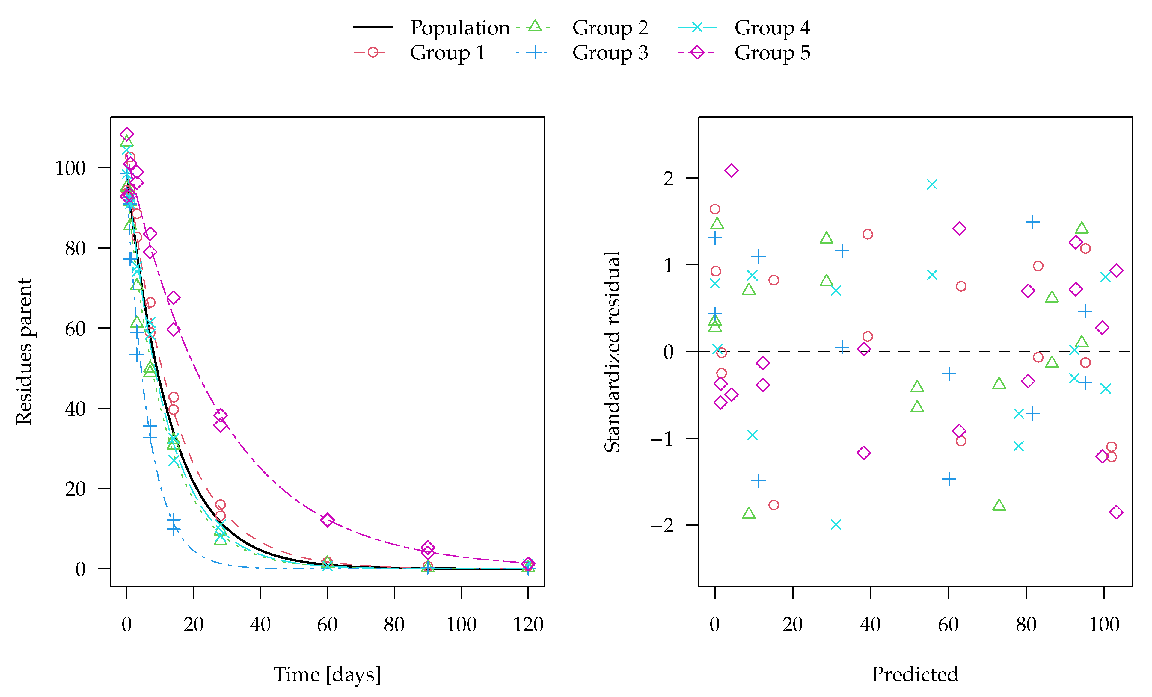
The evaluation of one of the 100 synthetic datasets generated for five virtual degradation experiments with half-lives centered around 15 days is shown in Figure 1. The residuals are standardised using the standard deviation predicted by the two-component error model at the respective magnitude of the predicted value. The corresponding fit using constant variance as well corresponding nonlinear mixed-effects model fits are shown in the Supplementary Materials. These look very similar, although in nonlinear mixed-effects models, the population mean curves are fitted first, the individual curves are estimated as empirical Bayes estimates in a second step and the standardised residuals are relative to those predictions. The residual plots in the right panels show a more random scatter when the two-component error model is used, as this is what was used to generate the data.

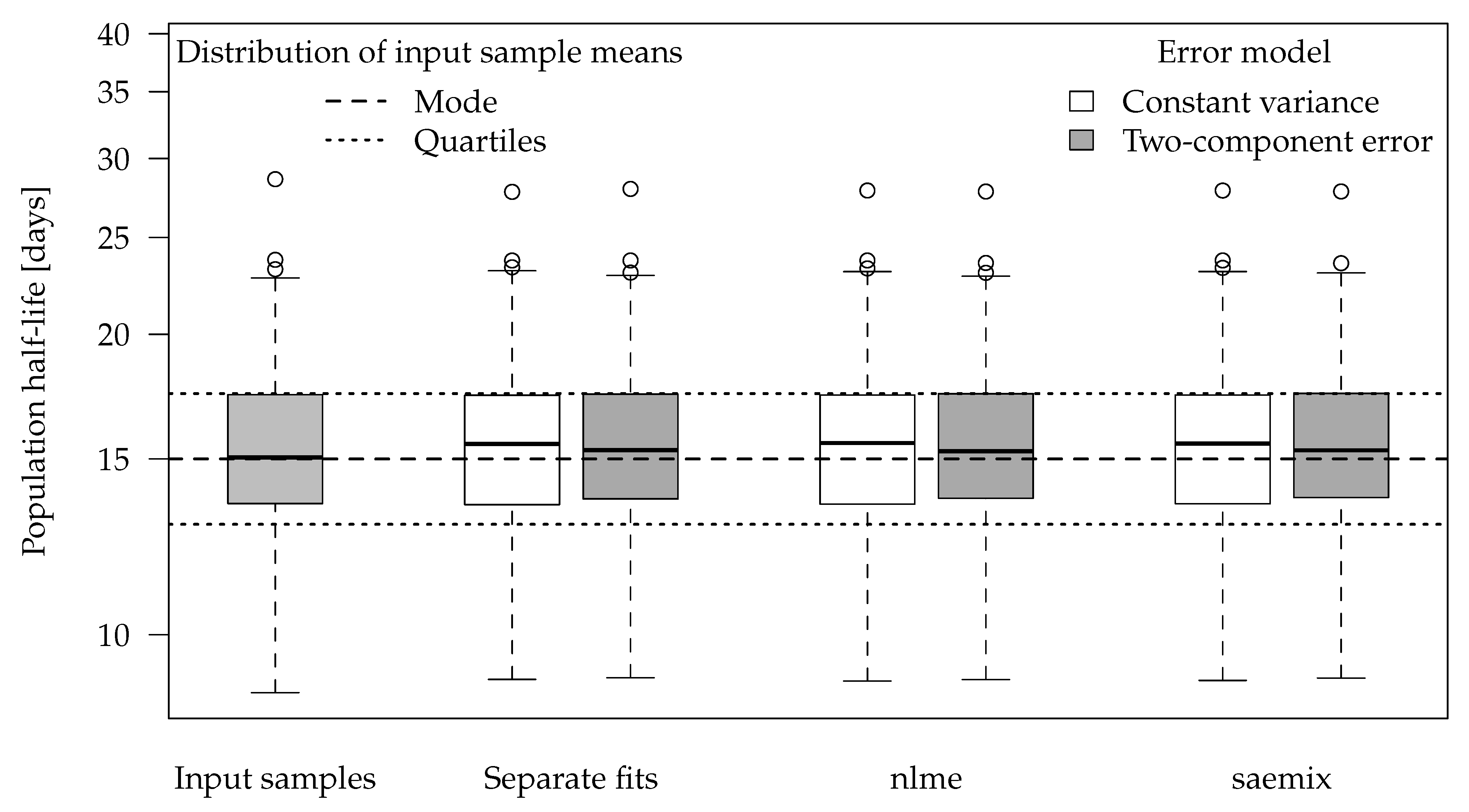
Figure 2 shows boxplots of the population half-lives for 100 synthetic datasets. For the data generation, five random half-lives were drawn from the log-normal distribution for each dataset (see the Theory and Methods section). The 100 geometric means of these samples are shown in the left-most boxplot. The boxes range from the lower quartile to the upper quartile. These can be compared to the theoretical quartiles (horizontal dotted lines) of the predefined input distribution. The differences are a consequence of the random components of the data.

For the separate evaluations, the geometric means of the half-lives obtained in the separate fits are shown. In the nonlinear mixed-effects model fits, the population half-lives are directly estimated.

The graph suggests that all six evaluation variants were able to recover the population means of the input samples reasonably well. This is also apparent from the half-live statistics over the 100 results obtained from each of the six variants presented in

Table 3. Statistics for half-lives derived from 100 synthetic grouped datasets with an input half-life of 15 days.

	Input		Separate Fits		Nlme		Saemix
	Distribution	Samples	const	tc	const	tc	const	tc
Number of results			500	500	100	100	100	100
Fits with lower AIC			11	489	0	100	0	100
Minimum		8.749	9.019	9.056	8.986	9.017	9.000	9.048
25th percentile	12.90	13.555	13.524	13.691	13.549	13.705	13.566	13.724
Median	15.00	15.053	15.530	15.312	15.563	15.272	15.544	15.303
75th percentile	17.44	17.358	17.326	17.382	17.336	17.416	17.346	17.438
Maximum		28.600	27.775	27.964	27.863	27.796	27.860	27.801

const: Constant variance; tc: Two-component error model.

.

Error model selection based on the Akaike Information Criterion (AIC) favours the two-component error model for 489 out of 500 separate fits and for all 100 simultaneous fits to these datasets, which confirms the visual assessment of the residual plots.

Synthetic datasets were also evaluated with half-lives centered at 120 days, 500 days and 800 days in order to explore the possibility to recover the known population half-life when the half-life is large compared to the last sampling time. The results for 120 days and 500 days are shown in the Supplementary Materials.

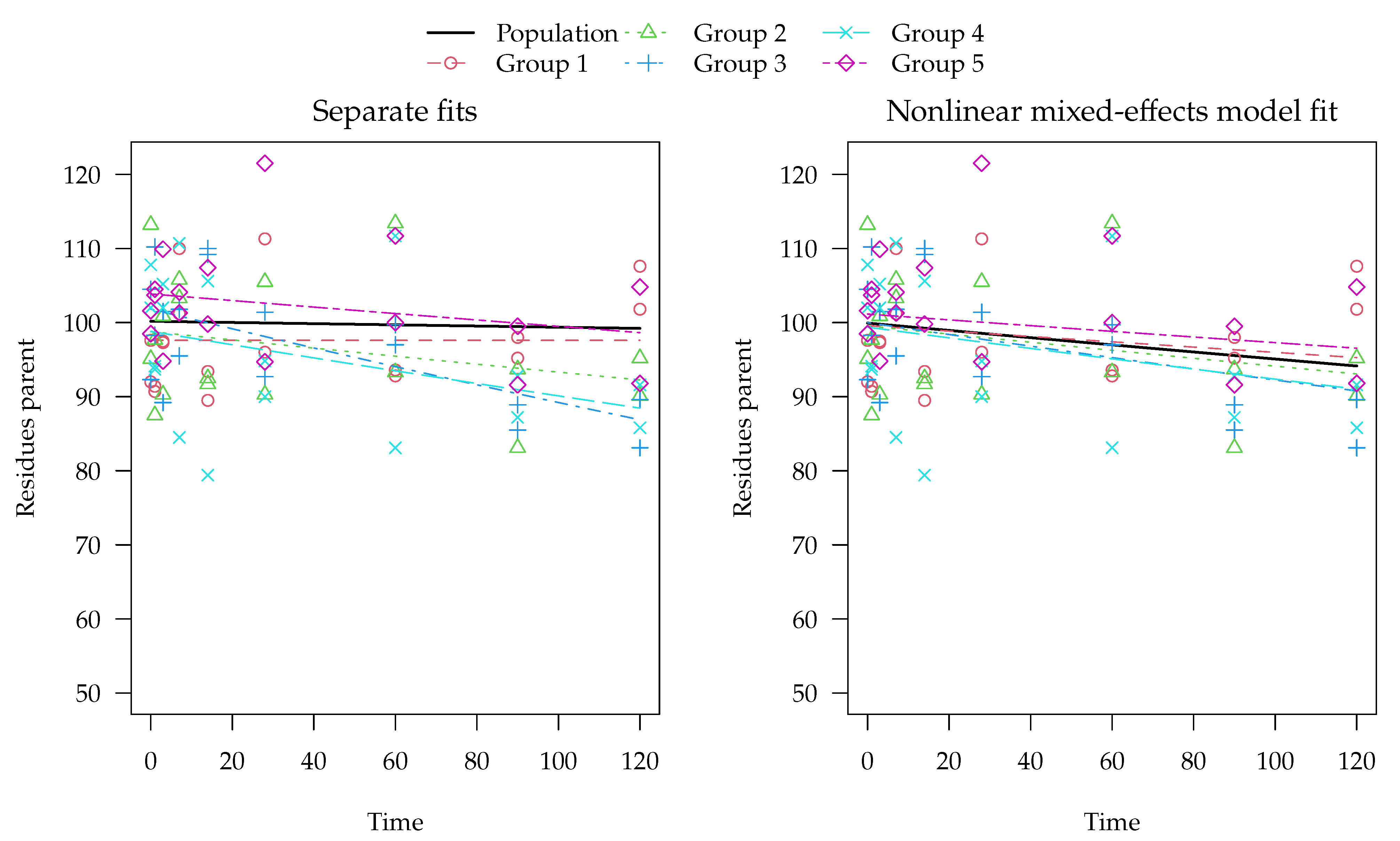
Separate evaluations with constant variance for one of the synthetic datasets generated with half-lives centered at 800 days are shown in in the left panel of Figure 3. Note that the example dataset in Figure 3 was selected as one of the 100 datasets where significant differences between the methods occur.

In this evaluation, an almost horizontal degradation curve was found for one of the groups (Group 1). The population curve resulting from simple averaging of log rate constants is also almost horizontal, although some visible degradation was found in the other four groups. The reason for this is that the geometric mean rate constant obtained from from these fits is still very close to zero because of the excessively low rate constant found for Group 1, which corresponds to a half-life of around 60 million days. Using the two-component error model did not improve the fit for this type of datasets (

Table 4. Statistics for half-lives derived from 100 synthetic grouped datasets, with an input half-life of 800 days.

	Input		Separate Fits		Nlme		Saemix
	Distribution	Samples	const	tc	const	tc	const	tc
Number of results			500	500	94	88	100	99
Fits with lower AIC			499	1	76	11	88	11
Minimum		480.4	438.1	424.4	408.6	407.6	440.3	430.0
25th percentile	688.0	657.3	683.5	678.9	604.2	595.7	648.8	647.0
Median	800.0	772.9	1029.7	852.7	690.7	701.4	761.3	756.5
75th percentile	930.2	897.8	6483.5	1381.7	841.7	865.2	1075.9	1029.2
Maximum		1401.2	856,749.0	444,191.3	4246.1	4260.1	57,459.9	2829.1

const: Constant variance; tc: Two-component error model.

).

The mixed-effects model fit obtained with saemix for the same example dataset is shown on the right hand side of Figure 3. Here, the population curve is not horizontal but shows a noticeable decline because it is determined by all data at the same time, so that ill-defined parameters in one of the groups cannot dominate the overall appearance of the curve.

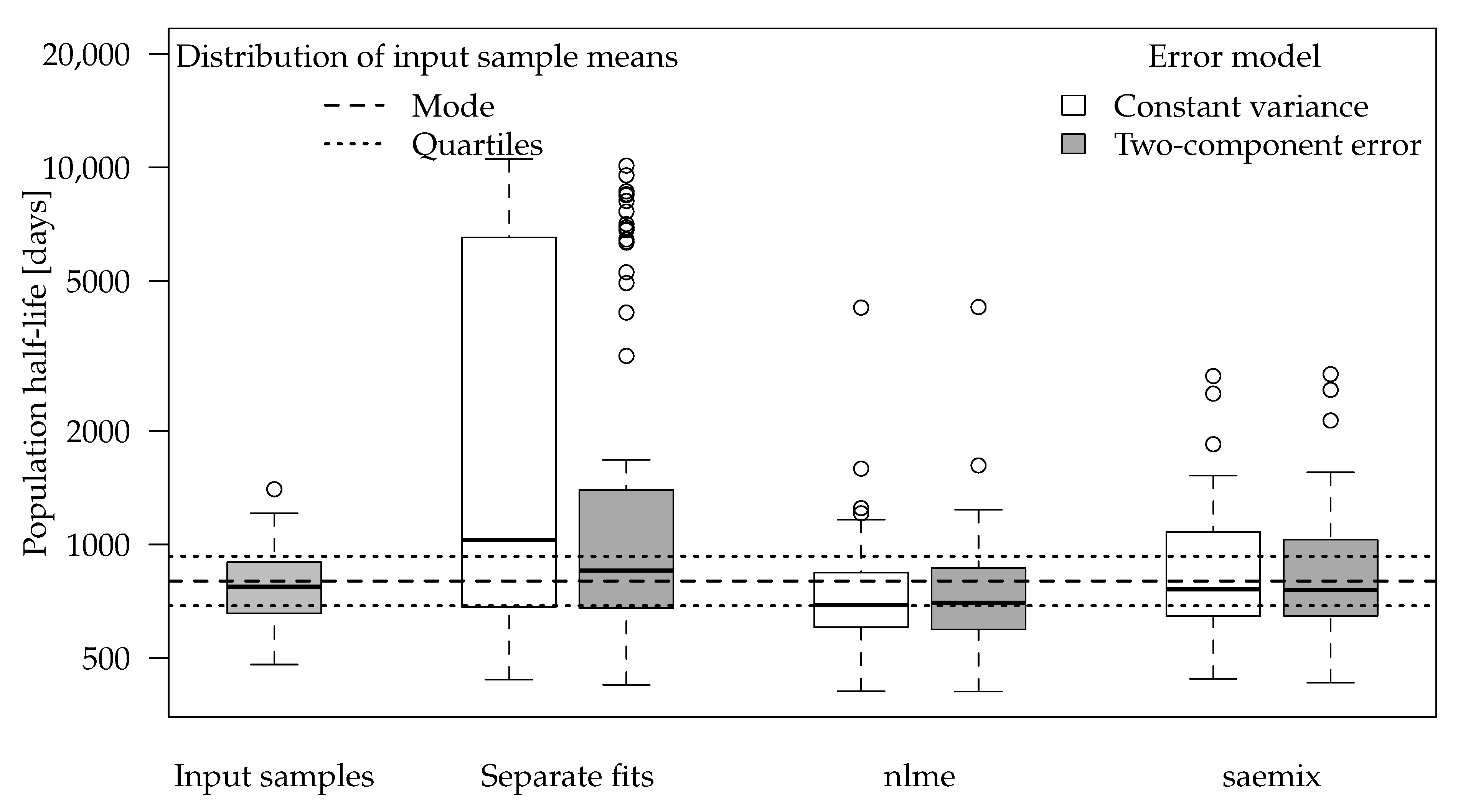
The boxplot for the population half-lives obtained for the input half-life of 800 days is shown in Figure 4. The number of successful fits and some statistics for the half-lives obtained by the different variants are shown in Table 4.

For separate fits, the input half-life is often not found with reasonable accuracy but rather overestimated as in the example dataset shown in Figure 3. The deviations are less pronounced when the error model matches the one used in the data generation process.

Population half-lives obtained using the nlme package show less overestimations. However, the algorithm did not converge for many datasets, so no results were available. Where the results were available, they showed a certain tendency to underestimate the half-life.

Fits using the SAEM algorithm were still able to recover the input population half-life in most cases. In one out of the 100 datasets, singularities in the Fisher information matrix indicated overparameterisation, so the corresponding results were not included. The affected dataset was also the one that yielded the largest overestimation of the population half-life in the separate evaluations.

In the datasets with an input half-life of 800 days, error model selection using the AIC would lead to selection of the constant variance fit in almost all cases for separate evaluations and in the majority of cases for the simultaneous fits (Table 4). This can be explained by the fact that the residues hardly decrease from the first to the last sampling times so that almost the same variance is used for the random data generation and the two-component error model is overparameterised. In general, using the two-component error model only slightly increased the accuracy of the population mean half-lives in these SFO datasets, judged by the comparison of the statistics given in Table 4.

The additional results for input half-lives of 120 days and 500 days shown in the Supplementary Materials show that the evaluation variants perform uniformly well for 120 days (with the exception of one case of non-convergence with nlme). In the case of 500 days for the input half-life, some cases of unrealistic population half-lives are obtained from separate fits and nlme shows a certain bias towards understimating half-lives, as the median as well as the first and third quartiles obtained in the fits that did converge are around five to ten percent lower than the known values. However, these observations were not as pronounced as for the data generated with a half-life of 800 days.

3.1.2. Synthetic Data for Biphasic Decline with One Transformation Product

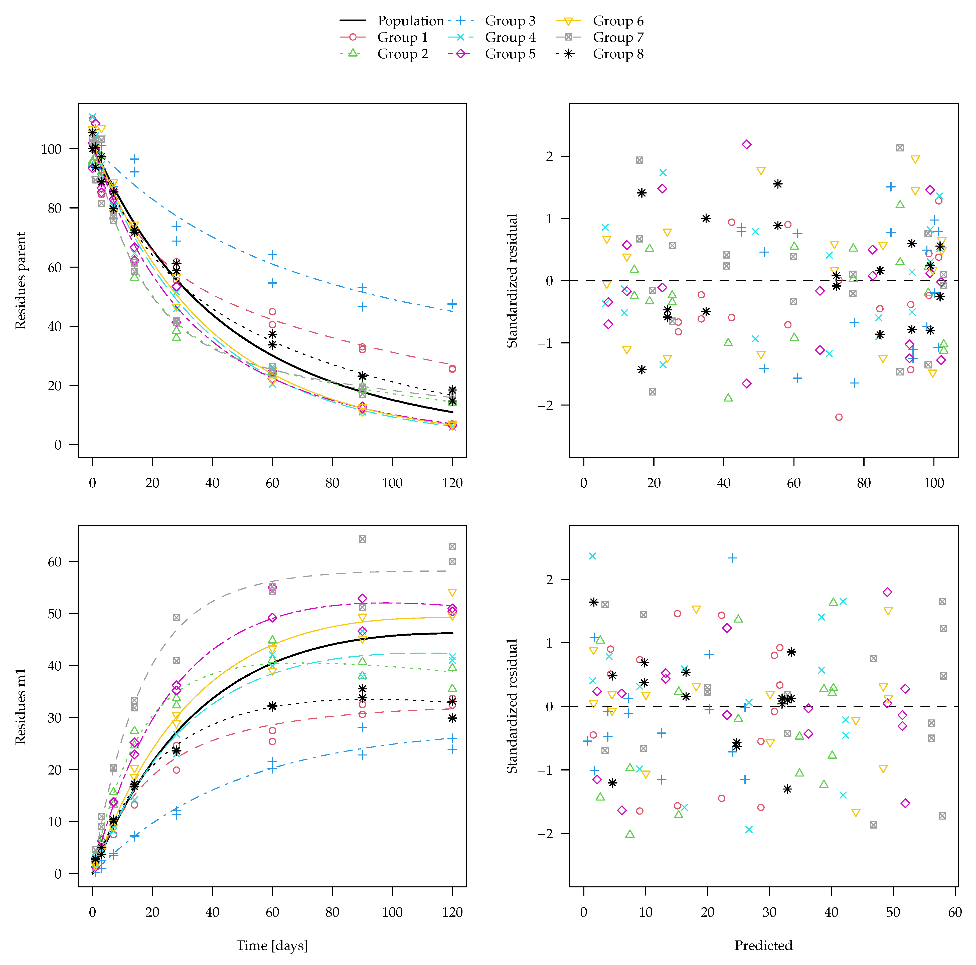
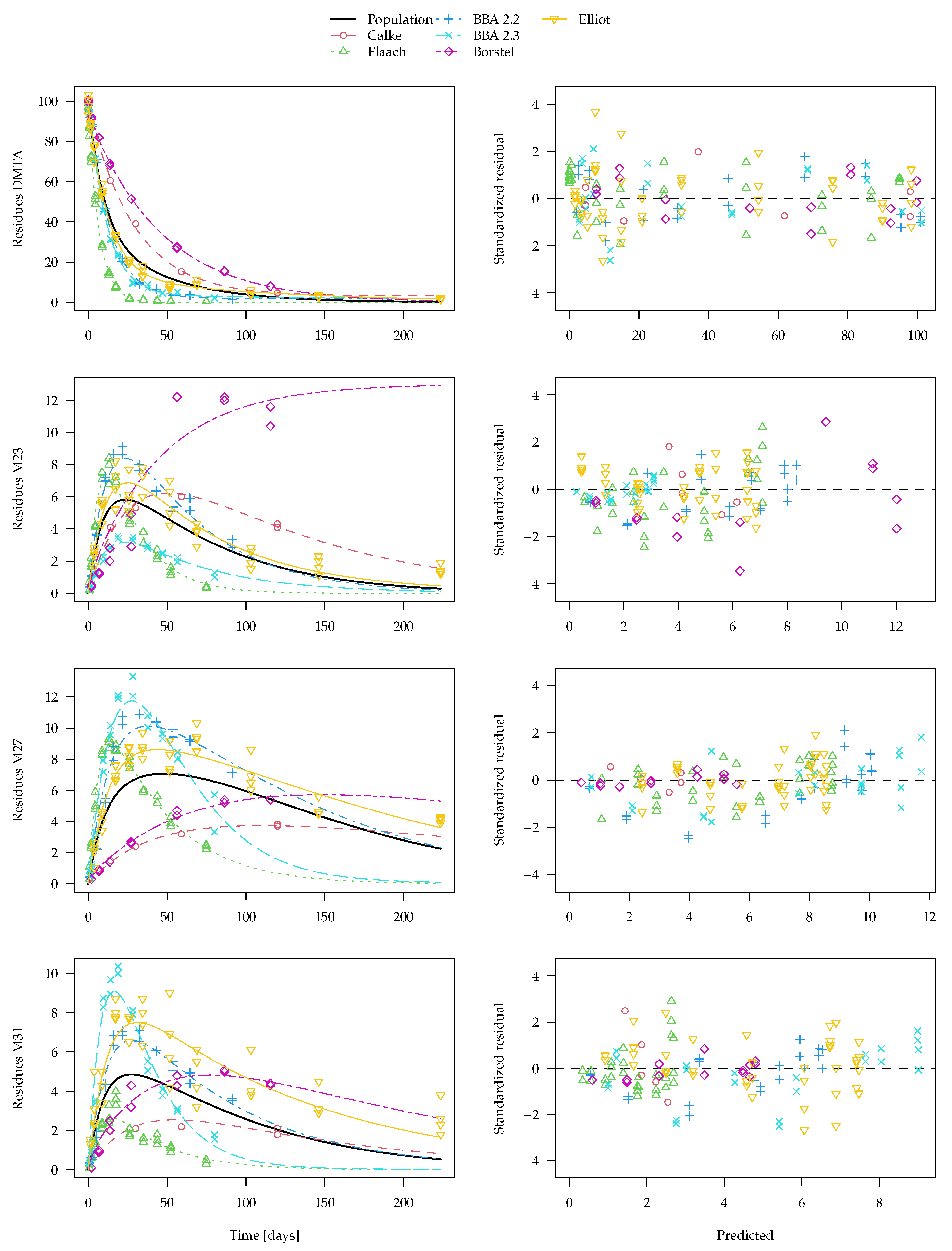
To illustrate the synthetic DFOP-SFO data, the nonlinear mixed-effects model fit with the DFOP-SFO and the two-component error model to one of the datasets is shown in Figure 5.

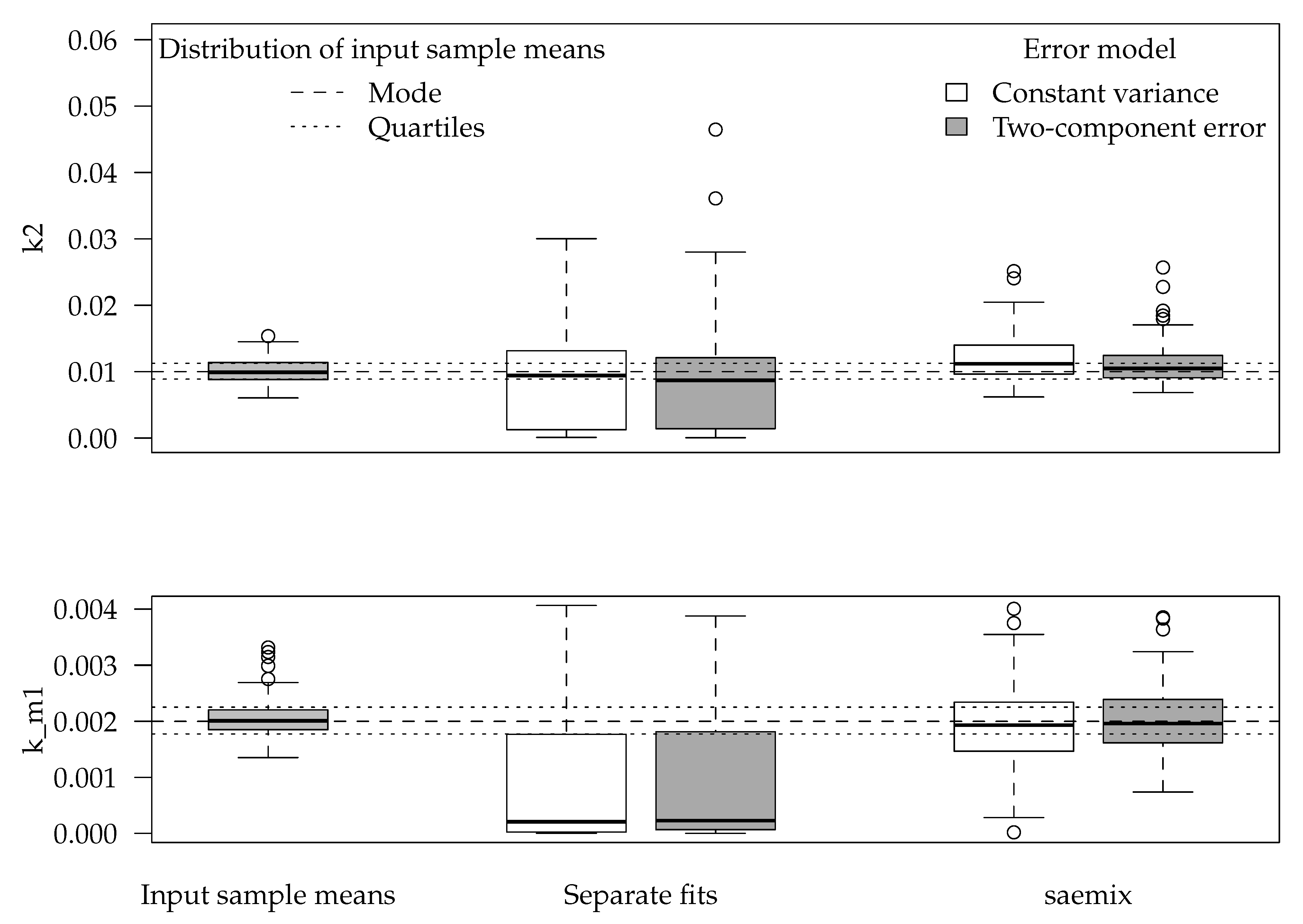
The boxplot for population parameters k2 (second rate constant of the DFOP model) and k_m1 (degradation rate constant of the transformation product) obtained for all 100 datasets using the DFOP-SFO degradation model and the two-component error model are shown in Figure 6.

The initial concentration of the parent compound, the faster parent decline rate constant k1, the DFOP parameter g as well as the formation fraction of the transformation product were recovered by separate and simultaneous fits with similar accuracy and without clear indication of a bias. The use of the two-component error model often led to smaller deviations from the known values. Boxplots for those parameters are shown in the Supplementary Materials.

For the slower parent decline rate constant k2, a large difference between separate and simultaneous evaluations was found. For the decline rate constant of the transformation product k_m1, this difference was even larger (Figure 6). For both parameters, the SAEM fit with the two-component error model resulted in the best agreement with the expected results.

3.2. Experimental Data

3.2.1. Experimental Data for 2,4-D and Two Transformation Products

A detailed documentation of the separate evaluations of the data for each soil according to the FOCUS guidance [3], including the kinetic model selection for each soil is shown in the Supplementary Materials. SFO kinetics were selected for the parent compound in all five soils. Based on the EU assessment, the degradation pathway is assumed to be linear from the parent compound to DCP, which further degrades to DCA. The model acronym SFO-SFO-SFO is used for this degradation model.

In two of the soils, the formation fraction from DCP to DCA is practically one. Therefore, a simplified degradation model without a formation fraction from DCP to DCA was additionally checked. In this model, there is no pathway from DCP to the sink compartment (CO₂, non-extractable residues or other, unknown transformation products). The acronym used here for this simplified degradation model is SFO-SFO(ns)-SFO, where the ‘ns’ in parentheses stands for ‘no sink’. The degradation rate constants obtained in the separate evaluations were normalised to reference conditions and their mean values were calculated as an estimate for the population of agricultural soils in the EU.

A number of alternative degradation model and error model combinations were fitted with nlme and with saemix. For nlme, only the fit of the simplified degradation model in combination with constant variance converged without adaptation of the control parameters. Out of the two variants for which convergence could be obtained, the reduced degradation model combined with the variance by variable error model gave the lowest AIC (see the Supplementary Materials for details). Only the results obtained with saemix are shown here.

In the fit of the full degradation model with constant variance parts of the Fisher information matrix used for the calculation of confidence intervals could not be inverted. However, when the two-component error model was used, the fit converged and this problem did not occur. The simplified degradation model without the pathway from DCP to sink was also fitted with saemix, but the full model was preferred based on comparison of the AIC values (see the Supplementary Materials).

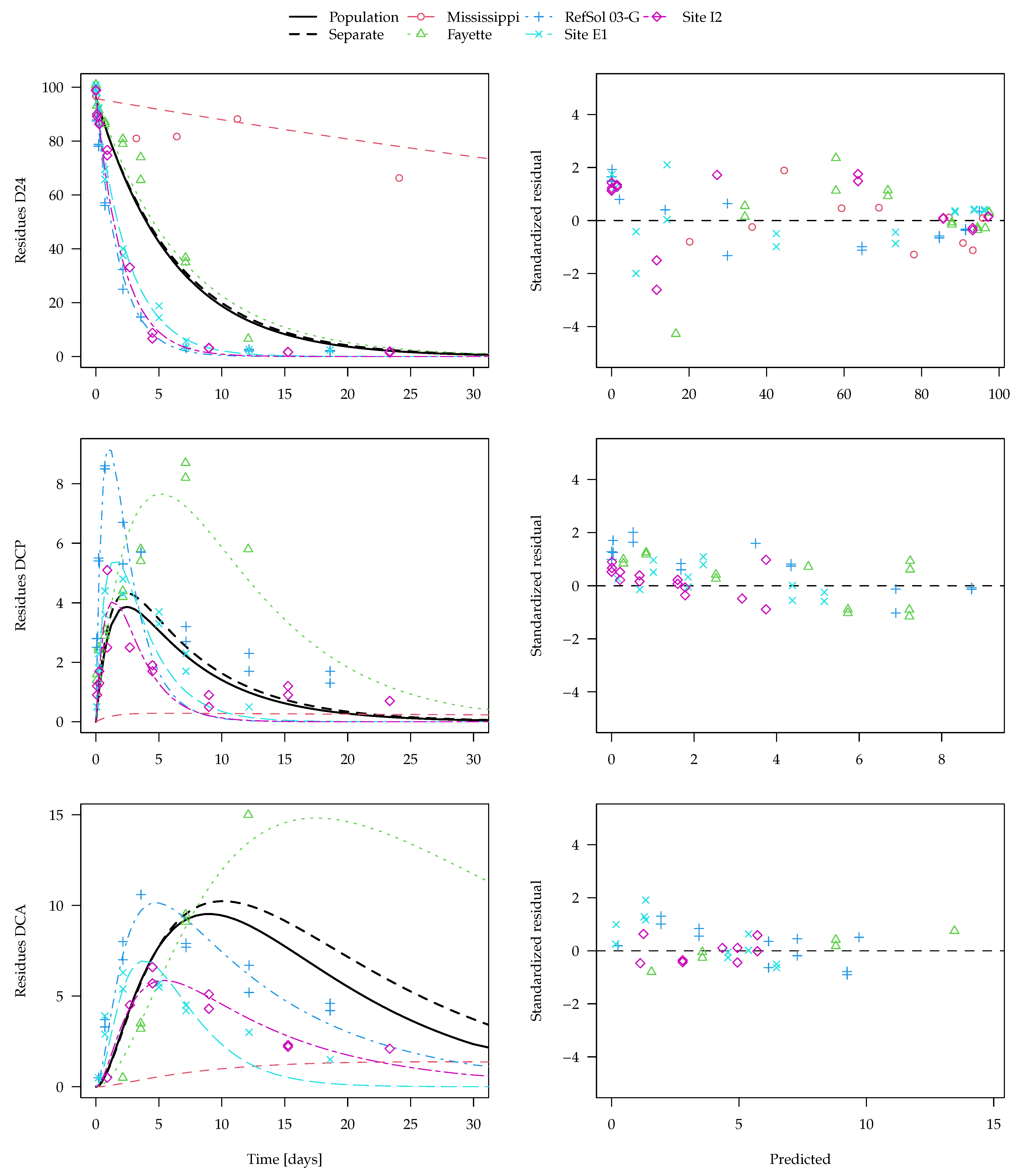
The population curve derived from the separate evaluations as outlined above is shown together with the best nonlinear mixed-effects model fit (SFO-SFO-SFO with two-component error) in Figure 7. Note that predictions for the transformation products DCP and DCA are even made for the Mississippi soil from the nonlinear mixed-effects model even though no experimental data for them are available. The x axis is limited to 30 days, as later observations are only available for the Mississippi soil. The complete plot of this fit and plots of other evaluation variants are shown in the Supplementary Materials.

Visual assessment of the available data suggests that it is quite far from an ideal situation, as the behaviour in the different soils is quite variable and the observation time does not cover formation and decline of the transformation products in all soils. Regardless of the evaluation method, more data would be needed to reliably assess the parameters of interest and their distributions. For the parent compound 2,4-D, degradation in the Mississippi soil is much slower than in the other four soils. Nevertheless, the parent degradation curves obtained for the population with the two different methods are hardly distinguishable in Figure 7. This is also true for the first transformation product DCP, where the population curve obtained from separate evaluations is very similar to the population curve obtained from the nonlinear mixed-effects model fit.

For the secondary transformation product DCA, the nonlinear mixed-effects model fit (solid black line) shows a smaller peak than the curve predicted from the separate evaluations (dashed black line). This can be explained by the fact that, due to a lack of data for later sampling times, the degradation rate constant of DCA in the Fayette soil cannot reliably be determined in the separate fits (see the large confidence intervals in the Supplementary Materials), which leads to a very small degradation rate constant compared with the other soils. The nonlinear mixed-effects model fit takes the degradation of DCA in the other soils into account and gives them a greater weight, as it is defined better by the data. Under the assumption that the soils are from the same population and that the degradation rate constant of DCA has a log-normal distribution, the nonlinear mixed-effects model fit is more realistic and should be preferred.

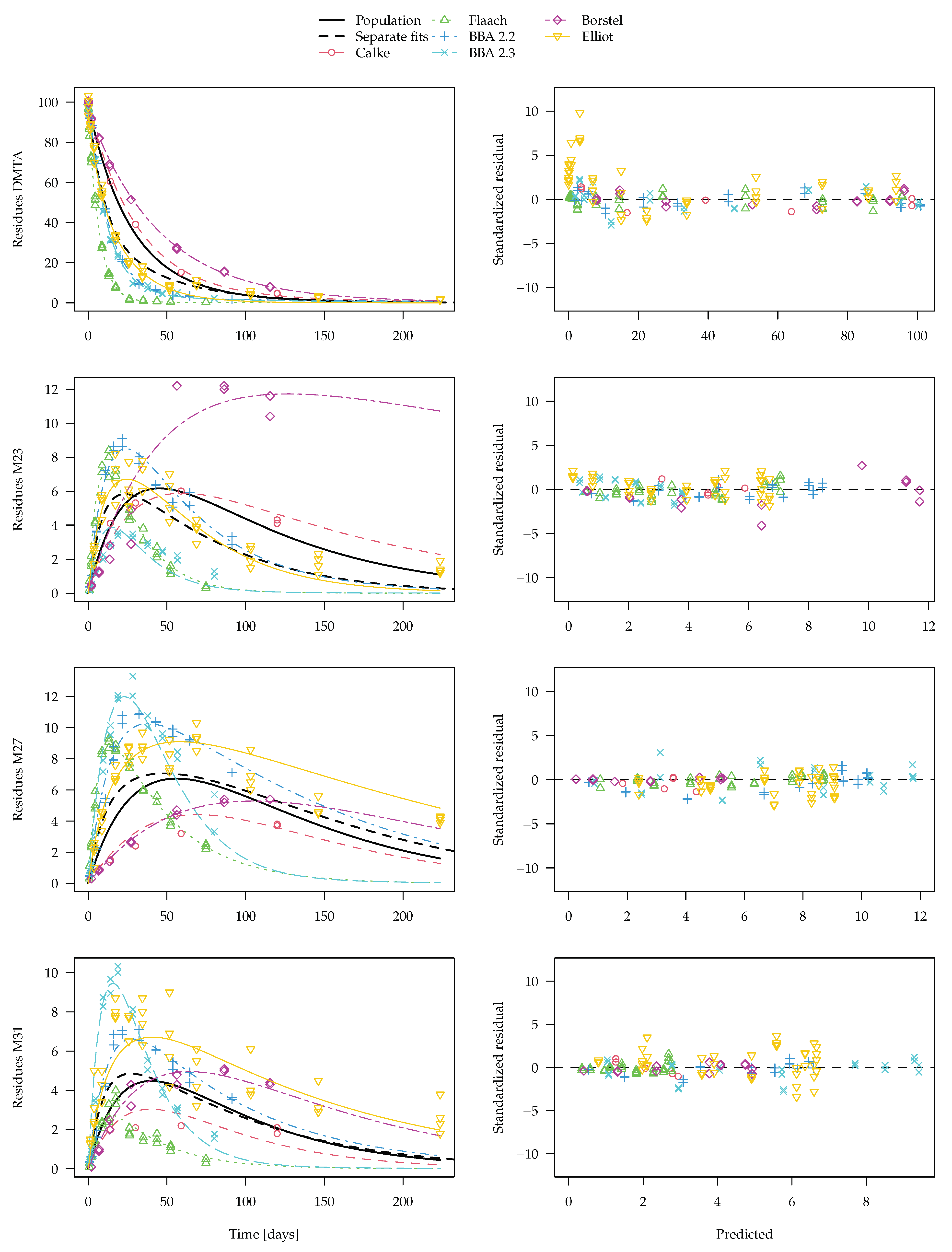
3.2.2. Experimental Data for DMTA and Three Transformation Products

The degradation model used in the EU review assumed parallel formation of these three transformation products, with SFO kinetics for all compounds. We use the notation SFO-SFO3 for this degradation model. In the EU evaluation, an additional pathway from M31 to M27 was assumed, with a formation fraction fixed to 1, which we denote SFO-SFO3+. Model selection calculations based on separate fits shown in tthe Supplementary Materials indicate that the additional pathway with fixed formation fraction slightly improves the fit in some soils while the simpler model is preferable in others. Even better fits could be obtained in the separate evaluations if biexponential decline was used for the parent compound (DFOP-SFO3 and DFOP-SFO3+) and if the two alternative error models were used. To obtain the lowest AIC in each of the six soils, four different combinations of degradation models and error models were necessary.

The separate fits for the DFOP-SFO3+ model with two-component error are shown in Figure 8. From this plot, it is clear that, for transformation product M23 as observed in the Borstel soil, no degradation can be determined in the separate evaluation. Therefore, the degradation rate constant determined for this fit is very close to zero and the t-test consequentially does not indicate significant difference from zero. Considering this rate constant in the calculation of a geometric mean degradation rate constant for M23 over all six soils results in a very small value. Similar problems occur in the separate fits of this model to the parent compound data. Since in some datasets, k1 or k2 are ill-determined, they can take on values that are very close to zero, which leads to nonsensical values when a geometric mean over all soils is calculated (a plot is shown in the Supplementary Materials). Therefore, the average curve shown in Figure 8 only considers rate constants that pass the t-test for significant difference from zero. However, while this curve does not look unrealistic, it does not take into account all available data. Therefore, the nonlinear mixed-effects model fit shown in Figure 9 should be preferred. The convergence plot for this fit shown in the Supplementary Materials indicates that convergence was reached. In the figure, the average curve from separate fits shown in Figure 8 is included for comparison.

For the parent compound, the averaging procedure leaving out rate constants that cannot be distinguished from zero leads to an overestimation of the degradation compared to the nonlinear mixed-effects model fit. As only the latter makes use of all available information, it is considered the more adequate representation of the degradation behaviour. A similar difference is observed for transformation product M23, where the degradation rate constant in the Borstel soil is not significantly different from zero and is therefore not taken into account in the generation of the dashed curve in Figure 9. The differences for the other two transformation products are less pronounced.

4. Discussion

The results obtained with synthetic data designed to resemble typical observed degradation data but with known statistical properties indicated that the application of mixed-effect models can more robustly and more accurately determine slow degradation rates representative of a population.

This was shown for SFO kinetics in cases where the degradation half-life was more than twice the duration of the virtual experiment. For shorter half-lives, geometric mean rate constants from separate evaluations performed equally well. However, it is not possible to specify a boundary half-life for when the use of nonlinear mixed-effects models will be superior because this depends on the overall variability of the data.

The population parameters describing the biphasic degradation of the parent compound and the degradation of a transformation product were also recovered more accurately when using nonlinear mixed-effects models. While the FOCE algorithm implemented in the nlme package sometimes showed a certain bias in population parameters, this was not the case when using the SAEM algorithm as implemented in the saemix package.

A more practical advantage can result from the fact that, for nonlinear mixed-effects models, model selection only has to be performed for the complete dataset and not for each individual dataset separately. While model selection also has to be performed for the parameter distribution models, these can be kept simple by assuming uncorrelated random effects, i.e., that the random variations of the parameters across the population are independent of each other.

The evaluation of experimental data also pointed to some practical limitations of the mixed-effects modelling approach tested in this work. In several cases, the FOCE algorithm implemented in the nlme package did not converge, which limits the use of this software in practical applications. When using saemix, fitting more complex degradation models with transformation products takes more time (around 10 to 15 min in our case) and may therefore disrupt the workflow if no analytical solution of the model is implemented. While this is certainly still acceptable, a factor limiting the general use of the saemix package is that it currently does not allow for different variances of the observed variables (variance by variable). This could be overcome by using other available implementations of the SAEM algorithm, for instance nlmixr [40] or Monolix [31,32].

In this analysis, we chose parameter transformations based on the natural parameter boundaries, i.e., log transformation for positive real parameters such as degradation rate constants and logit transformation for fractions. For degradation rate constants, using the log transformation reflects common practice in pharmacokinetics and reflects the practice of computing geometric means from several individual soil degradation rate constants in the separate fit analysis. However, the transformations cannot be reliably tested given the small number of data available in this study. Using a larger number of individual datasets, we could explore the distribution of individual parameters, test the influence of covariates linked to soil characteristics such as pH or organic carbon content, or assess departure from log-normality using different transformations h. Petersson et al. [41] suggested systematically testing transformations such as the logit distribution or the Box-Cox transformation to detect skewness, heavy-tailed distributions or even multimodalities in the parameters. It is inherently difficult to check the assumptions about the shape of the parameter distributions and the assumption that the experimental units are representative samples of the population of interest [42]. However, these problems are also present in the current approach based on separate evaluations as outlined in the respective kinetic guidance documents. We consider it an advantage that these assumptions are explicit when using nonlinear mixed-effects models because, in this way, models using different assumptions can be checked against each other.

Extensive diagnostic plots are available to check the various components of the model, going beyond the residual plots we presented here for comparison with the separate fit approaches. Such plots are simulation-based diagnostics that compare prediction intervals for given percentiles of the response to the observed percentiles. A tutorial on diagnostic plots can be found in Nguyen et al. [43].

5. Conclusions

Based on data generated with predefined statistical properties, it could be shown that, using nonlinear mixed-effects models, reasonable results can be obtained even in cases where degradation of the parent or a specific transformation product is very slow in some of the individual datasets. In addition to this exercise showing the advantages of the method in a controlled setting, the evaluations of experimental soil degradation data for two different pesticidal active substances showed that plausible results could also be obtained in cases where the conventional approach based on separate evaluations suffered from severe problems due to the lack of identifiability of certain parameters in specific individual datasets.

An additional advantage of the use of nonlinear mixed-effects models is the simplification of model selection, as this does not have to be performed for each individual group of data but only once for the complete dataset.

These results may allow us to replace the current use of arbitrary default values for datasets giving ill-defined results. Furthermore, the shift in model selection from the individual datasets to the level of the complete data has the potential to significantly reduce the number of model comparisons while allowing us to assess the influence of covariates such as soil pH in the same step. The proposed use of likelihood-based model selection criteria such as the likelihood ratio test and the AIC also has the potential to overcome excessive and unpredictable discussions about visual acceptability assessments.

While we cannot recommend the nlme package for the more complex degradation models as it often does not converge, the SAEM algorithm as implemented in the saemix package proved to be a reliable tool for fitting nonlinear mixed-effects models.

For routine use in regulatory degradation kinetics, either the variance by variable error model could be implemented in saemix or one of the existing alternative nonlinear mixed-effects modelling packages could be used. If possible, the execution speed of the ODE-based degradation models should be increased and a wider range of analytical solutions should be implemented. To facilitate wide adoption, some more effort is still needed to provide kinetic modelling tools that are versatile and easy to use for professionals working in this area.

Nevertheless, the theoretical background and the practical applicatons shown here give rise to the expectation that nonlinear mixed-effects models could be a cornerstone of chemical degradation kinetics in the future.