Article

Empirical Modeling of Stream Nutrients for Countries without Robust Water Quality Monitoring Systems

1
Laboratorio de Desarrollo Sustentable y Gestión Ambiental del Territorio, Facultad de Ciencias, Instituto de Ecología y Ciencias Ambientales, Universidad de la República, Montevideo 11400, Uruguay
2
Departamento de Ecología y Gestión Ambiental, Centro Universitario Regional del Este, Universidad de la República, Maldonado 20000, Uruguay
3
Centro Universitario Regional del Este, Polo de Desarrollo Universitario Modelización y Análisis de Recursos Naturales, Universidad de la República, Rocha 27000, Uruguay
4
South American Institute for Resilience and Sustainability Studies (SARAS), Bella Vista, Maldonado 20200, Uruguay
*
Author to whom correspondence should be addressed.
Environments 2021, 8(11), 129; https://doi.org/10.3390/environments8110129
Submission received: 21 October 2021 / Revised: 15 November 2021 / Accepted: 16 November 2021 / Published: 19 November 2021

Abstract

:
Water quality models are useful tools to understand and mitigate eutrophication processes. However, gaining access to high-resolution data and fitting models to local conditions can interfere with their implementation. This paper analyzes whether it is possible to create a spatial model of nutrient water level at a local scale that is applicable in different geophysical and land-use conditions. The total nitrogen and phosphorus concentrations were modeled by integrating Geographical Information Systems, Remote Sensing, and Generalized Additive and Land-Use Changes Modeling. The research was based on two case studies, which included 204 drainage basins, with nutrient and limnological data collected during two seasons. The models performed well under local conditions, with small errors calculated from the independent samples. The recorded and predicted concentrations of nutrients indicated a significant risk of water eutrophication in both areas, showing the impact of agricultural intensification and population growth on water quality. The models are a contribution to the sustainable land-use planning process, which can help to prevent or promote land-use transformation and new practices in agricultural production and urban design. The ability to implement models using secondary information, which is easily collected at a low cost, is the most remarkable feature of this approach.

1. Introduction

The excessive nutrient enrichment of water ecosystems, or eutrophication, is considered to be the main water quality problem at the global scale, restricting the sustainability of environmental goods and services [1,2,3,4,5,6]. Human actions have intensified eutrophication problems through drastic modifications of exchanges between land and water ecosystems. In particular, due to the increasing input of limiting nutrients linked to land-use transformations, such as phosphorus (P) and nitrogen (N) [7,8], agricultural expansion and the rising intensification of production have been impacted in recent decades [9,10,11].
Controlling the increasing nutrient inputs from point and nonpoint sources is essential to avoid the contamination of aquatic systems, and it is a first step toward rehabilitating or restoring eutrophic systems. Progress in nonpoint source control has been modest due to: (a) the complexity of quantifying and controlling inputs [12], (b) the diversity of mechanisms involved in generating nutrient outputs, and (c) the existence of resilience mechanisms (legacy) that maintain the consequences of processes even when fertilization has been diminished [13,14]. Based on the current trends of the expansion and intensification of agriculture and population growth, nonpoint source pollution will multiply and, consequently, the impacts on water quality will increase [15,16]. Therefore, controlling the nonpoint loadings of nutrients is urgently required [7,9,17].
Improvements in monitoring in terms of quantity, frequency, variables, automatic systems, and nutrient export estimations (e.g., [17,18]) have allowed the development of sophisticated water quality models (i.e., QUAL2E [19], SWAT [20] ARMF [21], HSPF [22], MIKE-SHE [23]). These models have greatly improved and their use has spread, particularly for the design of management strategies to reduce the nutrient exports into water systems [24,25,26]. In addition, nutrient models have emerged as essential tools to understanding the hydrological behavior of drainage basins in response to present and uncertain future anthropogenic pressures, such as land-use change and climate change [27]. Numerous models with deterministic and process-based modeling approaches have been used to evaluate various hydrologic processes (i.e., [28,29,30]). These models are based on the application of physical laws that are able to explain the main natural systems’ processes and have proven to be suitable for representing them at the catchment scale [30]. However, the fact that the model is based on physical laws does not necessarily guarantee good results [30]. In addition, acquiring and processing sufficient complete, valid and systematic data, as well as the complex calibration and adaptation of models to local conditions [12,31,32,33,34], are long-term challenges that demand significant economic resources [35]. Therefore, the construction of local low-cost models is a current need in water management, especially for countries with severe limitations to generate sufficient data to developed functional models. Empirical modeling is a promising alternative strategy to explore as it has yielded good results at local scales [36,37,38].
Building models with available spatial information finds new opportunities through the application of Machine Learning (ML) techniques, the integration of Geographic Information Systems (GIS) and Remote Sensing (RS). These alternatives are suitable for use in eutrophication control, specifically for land-use planning, water treatment, and fertilization systems design [34]. ML techniques provide a powerful set of tools that could contribute to the advancement of both explanatory and predictive models [39,40]. Among ML methods, General Additive Models (GAM) stand out, as they can be integrated with GIS to solve spatial problems [41]. GAM and GIS have a high potential to work with possible future scenarios (e.g., climate and land use). The Land Changes Modeler (LCM) has been broadly used to analyze and predict land cover transformations [42,43,44,45,46]. This type of model is widely applied to evaluate the role of each driver in land-use transformations. The prediction of land-use change is based on an empirical process, which begins with the analysis of past changes, followed by the modeling of the potential transition, and, finally, the resulting change [44].
In countries that are currently developing their water quality monitoring systems and applying models such as SWAT [20], which requires significant efforts—to address data gathering, calibration and validation—the following questions emerge: Can the available spatial watersheds data—edaphological, geomorphological, geological, climatic and land-use information—be useful to predict the nitrogen and phosphorus levels according to the combination of GIS, RS, GAM and LCM considered? If so, how relevant is the combination of different approaches such as GIS, RS, GAM and LCM for the land-use planning, prevention, and control of eutrophication processes? Answering these questions is the first step towards progressing in the management and conservation of aquatic systems, land-use planning, and the transition of productive systems and associated practices towards sustainable scenarios. This situation is remarkable in Latin America and calls for new strategies to gather information applicable to water management in the short term.
In this context, this work’s main objective was to model the nitrogen and phosphorus levels in lotic systems by combining GAM, GIS, RS, and LCM. The following hypotheses were formulated: (i) a high proportion of spatial variability of nitrogen and phosphorus levels in the water can be predicted using empirical models with available spatial information; (ii) if (i) is not rejected, this work’s methodological approach can contribute to the water management and land-use planning, while more robust models are built.
The models were developed and tested for two cases studies in Uruguay, with contrasting geophysics and land-use characteristics. Subsequently, the performance of the generated models and their ability to predict the spatial distribution of nutrient in the water were evaluated. Finally, the article assesses the strengths of this approach, its potential for land-use planning and water resource management, and the challenges ahead.

2. Materials and Methods

2.1. Research Strategy

Empirical probabilistic models are built with the aim of predicting response variables (nutrient levels) from predictor variables. The predictor variables were selected from a well-known causal mechanism (e.g., soil type, land use, geomorphology, key water channel processes such as in-stream oxygen levels) and spatial information available in Uruguay. The links between the two types of variables are known in theoretical terms, but not the contribution of each driver when analyzing the spatial variation of nutrients in the water in Uruguay’s geophysical and socio-economic context. To test the strategy, two contrasting case studies were selected. In both cases, spatially robust water quality monitoring programs exist, an uncommon condition in other Uruguayan watersheds. This allowed us to establish the ability for extrapolation of nutrient levels in the rest of the territory where there are currently no water quality monitoring programs. For this purpose, two extreme periods in hydrological conditions and the productive agricultural calendar of Uruguay were considered. In sum, a period of higher flows, lower temperature, prior to the beginning of the spring and summer crop cycles (winter–spring—WS—transition) and the opposite conditions in the summer–autumn (SA) transition.
A conceptual model was built to determine and evaluate the incidence of a group of potential causal factors of total phosphorus (TP) and total nitrogen (TN) levels in lotic systems. Second, a mathematical model was generated to identify the relationship between the selected drivers (predictor variables) and the TP and TN concentrations in water (response variables) in two case studies. The nutrient levels and other physical and chemical parameters were measured during WS and SA—in 2008–2009 for Case 1 and 2015–2016 for Case 2. The drainage basins of each water data collection point were defined as units of analysis to evaluate the connections between the TP and TN concentrations, structural attributes (type of soil, geomorphology, slopes), and land uses. A mathematical model was generated by integrating the following three stages:
  • The definition of natural and anthropic-originated (geophysical and land-use variables) controls that determine the levels of TP and TN concentrations in water.
  • The development a GIS for the systematization, evaluation, and integration of the controls (variables) identified in stage one to the 204 monitoring points distributed by the WS and SA periods.
  • The analysis of the relationships between controls and the TP and TN concentrations in lotic systems. The modeling was accomplished using GAMs.
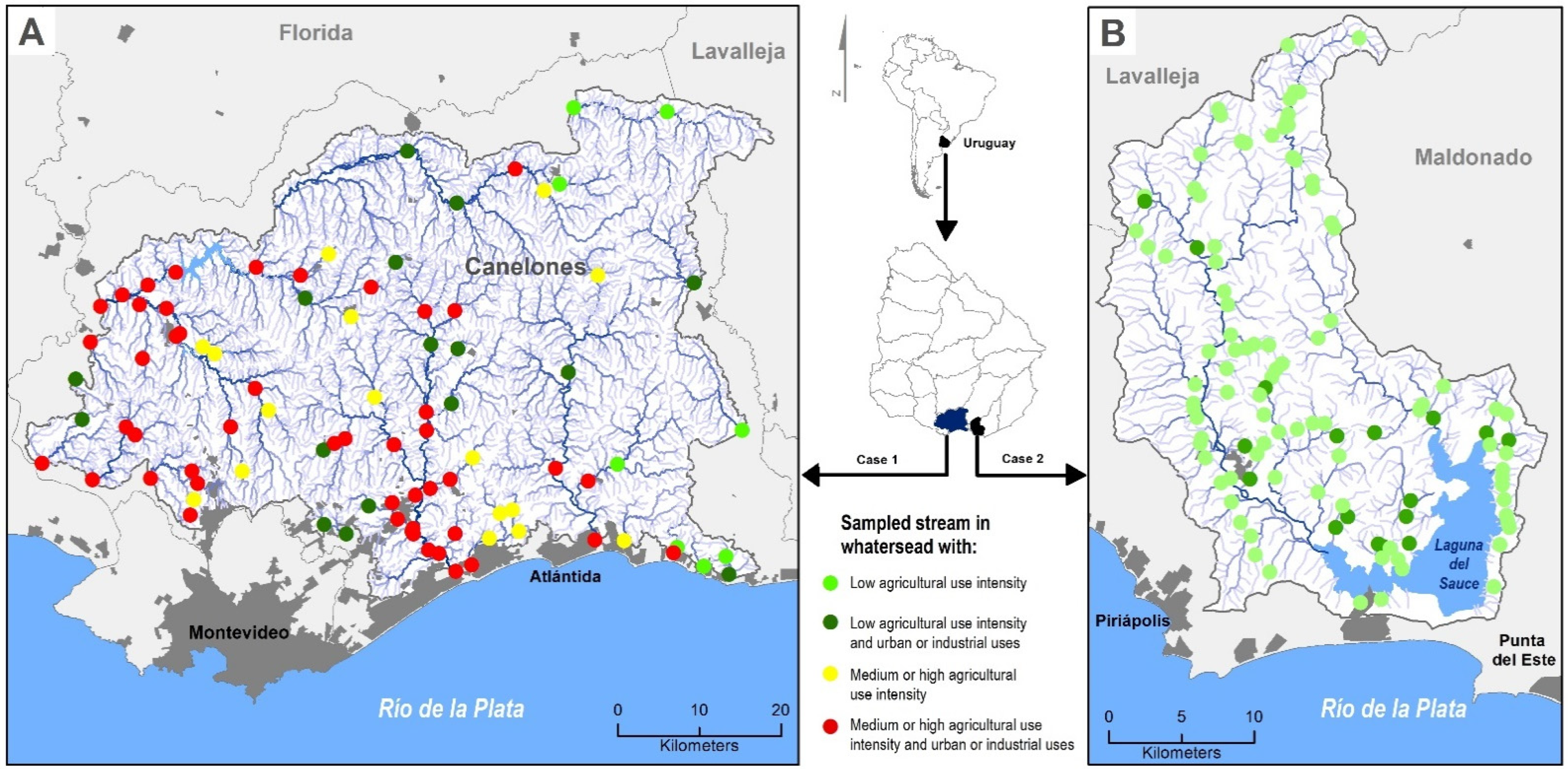
Last, the future water quality scenarios were evaluated using the model generated in stage three, adding information from an LCM and projected population growth for 2030.

2.2. Case Studies

Two case studies were conducted (Figure 1), as they present contrasting geophysical and land-use characteristics [47], and are strongly involved in water supply for human consumption. Combined, the area of both case studies provide freshwater for around 70% of Uruguay’s population. The climate in both areas is humid and temperate, with an annual rainfall over 1100 mm and an annual average temperature of 16.4 °C.
Case 1. Located mostly in Canelones and Lavalleja (Figure 1A) in south Uruguay, has an area of around 349,000 ha, which is subdivided into 87 hydrographic basins (average area: 13,631 ha; minimum area: 200 ha; maximum area: 77,000 ha). Hills are the dominant landform, with slopes under 6%, and the soils are highly fertile [48]. The most common land uses in rural areas are intensive agriculture and livestock production. This area shows high levels of anthropic soil erosion caused by human production throughout history. The urban population is 250,000 inhabitants, while in rural areas, it is approximately 41,000 [49]. The majority of towns and cities do not have traditional sewage systems [50]. In total, 74 agro-industrial complexes were registered, generally located in most densely populated areas.
Case 2. The Laguna del Sauce basin (Figure 1B) in Maldonado is located southeast Uruguay. It has an area of 70,743 ha, with a broad tributary network. A total of 117 sites were sampled, therefore 117 micro-basins were delineated (average area: 1,558 ha; minimum area: 571 ha; maximum area: 31,107 ha). Most of its surface is covered by natural pasture (53.9%), followed by afforestation (15%). Cattle farming dominates the primary sector activity in the area, with forestry and agriculture in second place. The urban and rural populations are 10,300 and 700 inhabitants, respectively [49]. Urban development intensification occurs near the water bodies, mainly for residential and touristic purposes.

2.3. Water Quality Data

For Case 1 (Canelones), the water quality data were provided by the Strategic Water Quality Plan for Canelones (PEDCA—IDC [51]) designed and implemented by the Canelones´ municipality. Two water sampling campaigns were performed in 87 sites. For Case 2 (Laguna del Sauce), data were collected in three consecutive sampling campaigns by Levrini [52] in 117 sites (Figure 1). In both cases, data were collected during the WS and SA transitions (2008–2009 in Canelones and 2015–2016 in Laguna del Sauce). The selection of sites aimed to cover the entire study area and account for the diversity of edaphological, geomorphological and land-use conditions, including water systems of social interest, environmentally relevant systems or areas, regions with high pressure on resources, paired micro-basins and location of nonpoint and point sources [51,52].
Through using a portable multiparameter sonde, conductivity (K), pH, and dissolved oxygen (DO) data were collected in the field. Water samples were taken below surface in the center of water channel and then filtered with GF/C Whatman. The resulting filters were dried at 100 °C until obtaining constant weight. Afterward, they were heated in a muffle furnace at 500 °C for 15 min and weighed again. The total suspended solids (TSS) concentration and suspended organic matter (SOM) content were estimated by weight difference [53]. With non-filtered samples, alkalinity was determined through titration with acid according to Wattenberg’s method [53]. The TP and TN concentrations were estimated from instantaneous-grab sampling using the simultaneous oxidation of phosphorus and nitrogenous compounds with the persulfate of potassium and specific spectrophotometric methods [54,55,56]. Analytic determinations were performed in Centro Regional del Este (UdelaR) the laboratories.

2.4. Land Use and Drainage Basin Characteristics

From the 87 samples corresponding to Case 1 and 117 to Case 2, an equal number of drainage basins were delimited through a digital terrain model (DTM) with 30 × 30 m resolution [57]. The database source used for modeling started with 13 variables, resulting in 18 parameters (Table 1). For each basin, a value for each parameter was extracted.

2.5. Data Analysis

The water quality parameters, geophysical attributes, and land use were initially analyzed for each basin using statistical univariate tests. Thereafter, Spearman’s rank correlation coefficient (ρ) was used to identify statistic relationships between these parameters. In the second stage, the existence of spatial dependency between sampling points was analyzed for each temporal period considered by Mantel’s test [67]. The tests considered the algorithms of Euclidean distance (ED) as the correlation (C) for the physical–chemical and geographical distance for the coordinate matrices. Mantel’s test proved the absence of spatial dependency. Therefore, this aspect was not considered when creating the model. In addition, the spatial patterns for water quality found in both the WS and SA transitions were analyzed using Mantel’s test. In this case, dissimilarity matrices (ED) containing a set of physical–chemical parameters for both periods were correlated. The analysis was performed using R software, version 3.6.1 [68].

2.6. Modeling

To model the relationship between predictor (land use and watershed geophysical characteristics) and response variables (TP and TN), a Generalized Linear Model (GLM, [69,70]) was initially applied. Thereafter, a GAM was used due to could perform better when there are non-linear relationships between variables [71] (Supplementary material (SM1)). The water nutrient level is controlled by several natural (i.e., soil type, parental substrate) and anthropogenic drivers (i.e., domestic effluent, agriculture). The GAM allowed us to identify the most important control factors that explain the spatial pattern of the observed water nutrients. One model is generated for PT and another model for NT.
In GAMs, as in GLMs, the components of the Y vector (response variable) are independent variables from an exponential family, this means that the random variables Y1,…, Yn are assumed independent and each Yi has a density function in the linear exponential family (e.g., Normal, Binomial, Poisson, Gamma, etc.)
The predictor and expected values of the response variable Y are related by a link function that must be monotonic and differentiable. GAMs have the following structure:
g(μ) = ß0 +f1(X1) + f2(X2)+ … + fp(Xp)
where g (the link function) is a known monotone differentiable function, μ is the expectation of the response variable, and functions fi(Xi) are smooth functions. These functions are flexible functions that adapt to the data and can be of several forms (cubic splines, natural splines, thin plate regression splines, etc.; for more detail of the construction of the smooth functions we refer to: [71]). It must be noticed that within one single model, different smooth functions can be considered to model the relation between different predictor variables and the response.
A total of 16 models were generated considering the different areas (Cases 1 and 2), nutrients (TP and TN), periods (WS and SA), and sections of the watershed. The two sections studied to understand nutrient dynamics of drainage basins were: (1) the drainage basin as a whole (section A), and (2) the in-stream processes (section B).
The final set of predictor variables in the models was defined according to Akaike’s Information Criterion (AIC; [70,72]) using a stepwise backward selection method [73]. In this method, the predictor variables are tested in an automatic procedure, and the variables that generate a model with lower AIC are eliminated through a stepped approach. The objective of this method is to reduce the set of variables and choose those that are most important to explain the response variable. With the aim to avoid multicollinearity problems, mainly in GLM models, in cases where the correlation between a pair of variables was greater than 0.5, only one of them was preserved.
The GAMs adjustment was performed using R software [68], applying the gam function from the mgcv package [74,75]. In all cases, the Gaussian family and identity link function were considered, maintaining the other parameters by default. Each model and all variables (response and predictor) used a transformation log (x + 1). This was necessary for the response variables to meet the model assumptions (normal and homoscedastic residue). For the predictor variables, the transformation was used because it significantly improved the model adjustment. The smoot functions thin plate regression spline [76] was used. The adequate adaptation of the dimension of the smooth functions base according to different predictors was checked using the function gam.check [74,75]. The gam.check function test whether the basis dimension (which is related to the degree of smoothness) for a smooth is adequate [77]. It computes an estimate of the residual variance based on differencing residuals that are near neighbours according to the (numeric) covariates of the smooth. This estimate divided by the residual variance is defined as k-index which is reported by the gam.check function. The further below 1 this is, the more likely it is that there is missed pattern left in the residuals, and then a higher basis dimension is recommended [77,78].
The goodness-of-fit measures were evaluated using the adjusted R2 and Generalized Cross-Validation (GCV, [79]) values. Both statistics were provided by the gam function. GCV is the model’s mean squared error estimator based on a crossed validation process: the leave-one-out type. Considering that GAMs tend to over-adjust data, the performance measurement was calculated on independent test samples to evaluate its predictive ability. The performance measurement used was the square root of the normalized mean squared error (NRMSE). Its calculation is as follows:
  • Data were randomly divided into two sets in a 90% training–10% test sampling proportion.
  • The training sample trained a GAM model with default parameters, and the test sample evaluated model adjustment with the training sample.
  • NRMSE (evaluation indicator) was calculated as Equation (1):
    RMSE mean ( Y )
  • RMSE refers to the square root of the quadratic error calculated as Equation (2):
    i = 1 n ( p r e d i o b s i ) 2 n
    where pred stands for predictor values for trained models on sample test data, and obs refers to values resulting from the response variable to the sample test.
Lastly, mean (Y) represents the response variable average in the sample test.
In total, 25 random partitions were made, and 25 values for NRMSE were obtained on the sample test. The purpose of doing several splits and averaging results was to avoid bias in NRMSE estimate related to one particular split [40]. These values were averaged to obtain the NRMSE average (±sd), which indicates the predictive ability of the models. The NRMSE was selected as an indicator due to: (a) it is easily interpretable (values close to zero indicate less residual variance), and (b) it allows easy comparison between models.

2.7. 2030 Scenario

A 2030 scenario was projected based on the assumption of rainfed agriculture (cereals and oleaginous) expansion, and the urban and rural population growth, following the ongoing trend of population growth since 2000 [63,78]. Additionally, productive strategies in the area, and urban and industrial source treatment systems were assumed to be constant for the studied period. The database considered for the LCM to project the agricultural and livestock uses for 2030 included the land-use classifications for the years 2000 and 2015, performed using the non-supervised classification of LANDSAT 5TM and LANDSAT 8OLI images and K-means clustering. The approximate area of agricultural and livestock growth was taken from Achkar et al. 2012 [79] and Uruguay’s Presidential Office of Planning and Budget [78].
Through the application of the LCM module [44], the probability of the transition to agricultural or livestock uses was analyzed from a spatial perspective for Cases 1 and 2. The variables under consideration were the soil suitability for agriculture, slopes, road distance, urban areas’ distance, and legal restrictions [50]. The agricultural and livestock projected areas of growth were distributed according to the detected areas with a greater probability of change. Finally, the values for each basin (sampling point) were integrated with the prediction model for the nutrient concentrations.

3. Results

3.1. Water Quality in Both Case Studies

In Case 1 (Canelones), most analyzed water quality attributes showed a high variation coefficient, indicating a significant spatial heterogeneity (Table 2). Significant pH gradients were found, most notably during SA, where the pH varied from very acid (3) to very basic (8.9) values, with a neutral pH mean for both periods. The conductivity (k) and alkalinity (Alk) presented moderately high values for both WS and SA, as well as an important spatial variability, especially for the K values (WS: 247, SA: 190.1 uS cm−1). The DO presented intermediate values during both periods, with higher variability during SA. The TSS concentration and SOM percentage displayed a broad spatial variability, particularly WS (170 mg/L and 71.1%). High nutrient concentrations were registered, with high spatial variability for both periods. The WS mean values of TN were greater than TP (5028 µg/L and 124.9 µg/L), while in SA, an opposite behavior was observed (816 µg/L and 2063 µg/L, respectively). Generally, the attributes presenting greater spatial variability were TN and TP, followed by K and the TSS concentration. This pattern applied for both periods, with higher variability during the WS transition. All analyzed attributes presented significant statistical differences between the studied periods. The values for TP and TN were highly correlated during WS (ρ = 0.69, p < 0.001) and SA (ρ = 0.73, p < 0.001). In addition, negative correlations were detected between TN and DO (WS: ρ = −0.43, p < 0.001; SA: ρ = −0.44, p < 0.001), and between TP and DO (WS: ρ = −0.37, p < 0.001; SA: ρ = −0.43, p < 0.001).
Case 2 (Laguna del Sauce) showed a diverse (spatially heterogeneity) tributary system in terms of physical–chemical properties, which was more visible during SA (Table 2). Significant pH gradients were registered, from acid (5.8) to basic (9.3), with a relatively neutral mean (7.2). K, as well as Alk, presented great spatial variability, with high mean values for both periods. The DO variability was low during both the WS and SA transitions, with similar mean values. The TSS concentration and SOM percentage showed variable spatial patterns, indicating water systems with a very low suspended matter (0.1 mg/L) and low SOM (0.1 mg/L), and systems with high TSS values (202.5 mg/L) and associated OM content (47.5 mg/L). The TN concentration presented very moderate mean values during both periods (WS: 503.7 µg/L and SA: 647.8 µg/L), with intermediate spatial variability. The TP concentration showed an important spatial variability in both periods (WS: 116.3 µg/L y SA: 210.4 µg/L). Overall, the attributes with greater spatial heterogeneity during WS period were TSS and TP, which increased during SA. The physical–chemical attributes that showed statistical differences between the WS and SA transitions were DO, TN, and SOM. The values for TP and TN were significantly correlated in both WS (ρ = 0.29 p < 0.001) and SA (ρ = 0.47, p < 0.001). An inverse relationship between TN and DO was observed during both periods. Finally, Cases 1 and 2 show partially stable spatial patterns between seasons. In addition, a lack of spatial dependency was noted for both cases.

3.2. Main Relationships between Nutrients and Land Use—Geophysical Variables

The TN and TP concentrations in Case 1 were mostly correlated with the land-use variables, especially with intensive agricultural, urban, and industrial uses (Table 3). As a general pattern, for both periods, correlation between TP and geomorphological and land use variables was greater than the correlation between those variables and TN. In Case 2, the correlations found between nutrients and geophysical variables were greater, as well as between water nutrients and non-intensive land uses, natural vegetation, and the state of riparian conservation.
In Case 1, excluding the drainage basins with point sources from the analysis, the correlations between the riparian areas and nutrients were significant during SA for both TP (ρ = −0.50, p < 0.0001) and TN (ρ = −0.32, p < 0.05), and during WS for TP (−0.28, p < 0.005).

3.3. Total Phosphorus and Total Nitrogen Models

The selected variables to elaborate the nutrient models were similar within each area (Case 1 and Case 2). The composition of the models differed more between area than nutrients (Table 4).
The models in Case 1 were built with a larger number of variables (six or seven) than Case 2 (four or five). In Case 1, variables linked to intensive land uses were included, such as point industrial sources, dispersed urban population, and rural population density. In addition, high-intensity rural land uses were included, such as orchard or crop production. Finally, livestock production, active soil erosion areas, and DO were included in the model. The models in Case 2 included less intensive rural land uses and did not include highly intense non-agricultural uses (e.g., industrial or urban uses). Case 2 also included the type of soil and conservation of riparian areas.
In both cases, the models, including section B (basin + in-stream), showed a greater correlation between the predictor and response values, lower NRMSE, and smaller AIC, except for TN in SA for Case 2 (Table 5). The models showed better performance during SA for Case 1 and for both nutrients. Similarly, during WS in Case 2, greater R2 for TP was registered than for TN, but at the same time, the error was higher. In general, the models’ performance fluctuated between 0.53 and 0.67 in Case 1 and between 0.3 and 0.54 in Case 2. The models that performed better for both nutrients displayed NRMSE values varying between 7.5% and 24.3%.

3.4. Total Phosphorous and Total Nitrogen Models Application for 2030 Scenario

For the 2030 scenario, a 20% growth and 160% growth in agricultural area is expected in Case 1 and Case 2, respectively, as well as a 7% population growth in both areas (Supplementary material (SM2)). These changes would increase the TP and TN concentrations in winter–spring and in summer–autumn (Figure 2) if the fertilization practices and domestic wastewater treatment remain unchanged. In Case 1, the TP growth would be 35% higher during SA than in WS, even though in relative terms, the growth would be even (15% in WS and 13% in SA). This growth was dissimilar among the 87 sampling points, as well as between both seasons (SA: VC = 119%, WS: VC = 112%). The average TN would increase two times more during SA (26% growth) than during WS (8%). The growth was also differential between the 87 sampling points (SA: VC= 89%; WS: VC = 151%). Considering the seasons (WS and SA) and sampling points, the projected growth of the TN and TP concentrations was not correlated (p > 0.05), indicating a spatially diverse increase for both nutrients. In Case 2, a similar expected growth of the TP concentrations was found in the SA (11%) and WS (10%) transitions. This increase would not be homogeneous among the different sampling points during SA (VC= 141%) and WS (VC = 98%). The TN average projected growth was higher in SA (7%) than in WS (2%), and showed variations between sampling points (SA: VC = 99%, WS: VC = 71%). In alignment with the Case 1 results, a spatially heterogeneous expected growth for both nutrients was registered between the seasons (p > 0.05).
As a general pattern for both areas, the TN concentrations in the 2030 scenario would increase at a higher rate in basins with lower current concentration values (Table 6). For TP, the same pattern was observed, except for SA in Case 1. In Canelones’ case, the projected increase in the TN and TP concentrations was mainly explained by the population growth (ρ = 0.57, p < 0.001; ρ = 0.73, p < 0.001), while in Case 2, it was associated with the agricultural growth (ρ = 0.51, p < 0.001).

4. Discussion

The approach that was carried out allowed the identification of the main drivers of nutrient levels in the water and to predict nitrogen and phosphorus levels in lotic systems. The application of the models under contrasting geophysical and land-use conditions delivered similar results in both cases. Thus, the models developed are a promising tool for applications in different social, economic, ecosystemic, and productive contexts. The tested models allowed the identification of natural and anthropogenic controls for the observed patterns, enabling them to guide the design of strategies and policies to control nonpoint sources, as well as research and action. Applying a predictive model for land-use changes and population growth provided another potential benefit for assessing water quality impacts and land-use planning.
Using GAM models made it possible to explain a substantial part of the spatial variability of TP and TN to a greater extent for both periods and case studies (Supplementary material (SM3)). GAM models, unlike GLM models, consider different types of relationships (i.e., linear or non-linear) between the response and predictor variables. In addition, the relationships can be of different types for each driver considered. In short, it is an alternative with greater potential if the system is composed of non-linear relationships or different types of relationships between response and predictor variables, a likely situation in study areas with significant environmental and spatial gradients. In addition, the models that included the dissolved oxygen concentration in the water achieved better results in all cases, indicating the importance of considering the internal processes within rivers and streams [82,83]. In summary, using GAM models with the combination of landscape attributes and water channel attributes (DO) increased the predictive ability of the nutrient’s models.
A positive association between the contribution of each driver to water runoff (steeper slopes and coarse-grained soils) and nutrient movement was detected [84]. However, the relationships do not entirely agree with the scientific literature (e.g., slopes and soil type). The spatial pattern of nutrients was conditioned by the spatial distribution of the land-use intensity, where intensive uses—which tend to account for higher TN and TP concentrations in soil—are in areas with favorable geophysical conditions (softer slopes, less degraded soils, fine-grained soils, etc.). On this basis, the land uses possibly mask the influences of the “structural variables”. The sign and the magnitude of the correlation’s coefficient found between the drainage basins’ attributes—geophysical and land use—and nutrient concentrations in both study areas allow us to support this hypothesis. The correlations were significantly stronger in Case 2 (non-intensive land uses) than in Case 1 (intensive land uses). No significant relationships were found for the other drivers (basin size, stream order, and other morphometric and morphologic features).
Geophysical variables should not be interpreted as less important than land-use variables. This implies that if intensive land uses are developed in other geophysical contexts (e.g., soils with stronger slopes, fine-grained and degraded), the nutrient concentrations results would be different, probably higher. For example, reestablishing the intensive production of several areas in Case 1 could unchain an extra input of TP for two reasons: (1) because of the system’s fragility and its predisposition to increased runoff (soil degradation and/or strong slopes), and (2) due to the available TP storage accumulated from previous agricultural uses [85] in the studied areas’ soils. Some aspects of the models should be highlighted, as that the empirical approaches do not imply that they cannot incorporate causal mechanisms. The strength of empirical models to identify the main drivers of a response variable—as in this work—is simultaneous with their limitations to model behaviors governed by processes that were not identified with a statistical approach. Other approaches, such as deterministic ones, have been successfully implemented in numerous cases (e.g., [29]) and could contribute to solve some of these problems. Deterministic models offer good results after the calibration of the variables and their application is supported with knowledge of modeling [86]. However, those models need the parameterization of the variables, which is often expensive, time-consuming and difficult to achieve. A major challenge lies in exploiting the advantages of both models. This would make it possible to understand processes with more precision [38], improve predictions, and generate a powerful tool to evaluate mitigation measures for specific conditions with no available precedent. This situation would make it possible to resize the role of structural variables. Considering these variables at a lower level of importance than land-use ones, could have serious impacts on water quality. The geophysical and land-use variations between both cases determined clear differences in the waters’ nutrient concentrations and marked distinctions in the models’ attributes. In the Case 1 model, the type of soil variable was not included, but point (industries) and nonpoint sources (rural population) were considered. The rural population density in Case 2 (1.0 hab/km2) was lower than in Case 1 (11.7 hab/km2), as well as the point sources, which determined a marginal impact of these actions as sources of limiting nutrients. Finally, the intensity of rural land use in Case 1 was twice that of Case 2, and the production was more diversified [47], which determined a lower inclusion of the land-use variables in Case 2 (e.g., orchard production).
The projected 2030 scenario would trigger an increase in the nutrient concentrations in water. This increase could intensify the already critical situation detected by the water quality sampling in Case 1, especially for TP. In Case 2, the increases would be lower than in Case 1. However, Laguna del Sauce is an ecosystem that is extremely sensitive to eutrophication (with severe interference to the drinking water supply due to cyanobacterial blooms) given its mean depth and residence time [87]. Hence, slight changes in land use could lead to a significant intensification of eutrophication.
In Case 1, the increase in the nutrient concentration in water did not correlate with agricultural growth. This pattern is likely to occur because: (i) the intensification of agriculture would be accompanied by an increase in other sources of nutrient export (increase in population and population density), (ii) the pattern of agricultural growth is not homogenous, and covers a large part of the study area, (iii) both factors may hide the role of agriculture as a nonpoint source of nutrients. In addition, the Land Use Planning Ordinance [50] may control and discourage agricultural expansion and therefore could reduce its impacts on water quality. In fact, the projected scenario already considers a significant area of exclusion for industrial agriculture in the Case 1 (SM 2). Simultaneously, the absence of correlations between the nutrient concentration and agricultural growth detected in Case 1 contributes to new evidence supporting the complexity of the area. We hypothesize that there is a legacy effect of abandoned or replaced agricultural systems and more point sources inputs—from urban and industrial areas—than nonpoint inputs.
In Case 2 (a less complex system showing less intensive land uses and smaller urban and rural populations), agricultural growth was the decisive factor determining an increase in the TP concentrations. An additional phenomenon to be studied is the expansion of afforestation (exotic species) registered in recent decades in Uruguay, a trend that is expected to continue. This variable was not included in generated models. Therefore, it was not included in the 2030 projection either. Since this change in land use would alter the hydrological behavior [88,89], it may promote an inferior dilution capacity and, ultimately, increase the risk of eutrophication during drier seasons.
The implemented approach allows for the generation of information for land-use planning at two scales—the drainage basin and region—and for two target resources: water and soil. At a drainage basin scale, it enables the identification of specific land uses in certain locations that may compromise water quality. At a regional scale—a group of micro-basins—it can contribute to the spatial planning design to ensure that changes in rural land use will prevent impacts on water quality. The expansion and intensification of Uruguayan agricultural production have been documented [90], and the most likely scenario is that this trend will continue. These models are a powerful tool to monitor the impacts of agricultural intensification on the water quality in each basin, a major input for assessing the impacts of land-use changes according to predefined water quality standards/criteria. This information is crucial in rural regions where land-use intensification is imminent (it only remains to decide precisely where), and where national agricultural policies promoting intensification must coexist in harmony with water resource conservation. Incorporating information about changes in agricultural practices into the model (i.e., tillage practice, fertilization and pesticide application methods), and upgrades in treatment systems (urban and industrial), will allow the assessment of different mitigation strategies, a key aspect of water resources management.
In the last two decades, several environmental regulations have been introduced in Uruguay (e.g., Decree Nº405/008—Land Use and Responsible Management Plan [91]). Nevertheless, the intensification and expansion of agriculture, livestock, and Eucalyptus forestry production [90] demands new approaches and regulations (especially nutrient input control). The interaction between environmental policies and agrarian intensification raises major uncertainties today. Integrating spatial models elaborated with planning scenarios could improve decision making process. The developed models can provide valuable information for new approaches, such as the construction of projected scenarios [92] for climate, land-use changes, land-use planning, and environmental policies.
The models developed in this research demonstrate that it is possible to obtain low prediction errors (NRMSE = 15 ± 6) and high correlation between predictive and response values (R2 = 0.53 ± 10) with data from open or available databases, information generated by remote sensing or geoprocessing, and without depending on excessive monitoring efforts after the initial sampling. However, several challenges related to the scaling, updating, and reliability of the data persist and could hinder the implementation of these models in Uruguay. The main challenge is to access up-to-date information generated at manageable costs.
The ability to implement models using currently available secondary information, or easily collected at a low cost, is the most remarkable feature of this approach. The generated models are a viable alternative for expanding our knowledge of ungauged Uruguayan aquatic systems.

5. Final Remarks

The combination of different approaches—GIS, GAM, RS, and LCM—shows that it is possible to develop efficient local spatial models, with a moderate data collection effort, to evaluate the nutrient concentration in lotic systems.
The developed models show the importance of land uses as the main drivers of nutrient concentration in the water, as well as the contribution of natural (structural) control factors. In addition, the models made it possible to determine the role of the key internal processes of the aquatic ecosystems, such as the dynamic of oxygen concentration, on a nutrient level.
The results suggest that for long-term solutions to water quality problems, it is essential create productive systems with nutrient balances close to zero or, in the most critical situations, negative. Similarly, there is still a need to improve the point source control and sewage system efficiency. Actions focused on the final phase of the nutrient export process—to implement buffer areas—could contribute to the reduction of nutrient input into water ecosystems. However, these actions will not be fully sufficient if the processes associated with agriculture in upper and medium drainage basins are not monitored and controlled.

Supplementary Materials

Author Contributions

Conceptualization, I.D., P.L., M.A., G.G. and N.M.; methodology, I.D., P.L. and C.C.; validation, I.D. and P.L.; formal analysis, I.D., P.L., C.C. and G.G.; investigation, I.D., P.L. and C.C.; data curation, I.D., P.L., C.C. and G.G.; writing—original draft preparation, I.D., P.L., N.M. and C.F.N.; writing—review and editing, I.D., P.L., M.A., C.C., C.F.N., G.G. and N.M.; visualization, I.D.; supervision, M.A., G.G. and N.M.; project administration, N.M.; funding acquisition, N.M. All authors have read and agreed to the published version of the manuscript.

Funding

This research was funded by CSIC-UdelaR (P.L Postgraduate scholarship), ANII (BE_POS_2010_1_2391 and FSDA_1_2018_1_154610), and PEDECIBA-Geosciences (P.L. scholarship). Water quality sampling in Canelones’ lotic systems was founded by the Intendencia de Canelones. I.D., M.A., C.C., G.G. and N.M were supported by the National Researchers System (SNI-ANII-Uruguay).

Institutional Review Board Statement

Not applicable.

Informed Consent Statement

Not applicable.

Data Availability Statement

The data presented in this study are available on request from the corresponding author.

Acknowledgments

This publication is the result of agreements between the Research Group on Ecology and rehabilitation of aquatic systems (Universidad de la República—Uruguay) with water supply company Obras Sanitarias del Estado (OSE-UGD-Maldonado) and the Canelones Municipality. In the name of Canelones Municipality, we especially thank to Leonardo Herou for your contribution to build links between academia and environmental management. Additionally, we warmly thank Sandra Acevedo and to all the workers of the above-mentioned municipality, who made this possible. Finally, to Soledad García Guarino and Claudia Fosalba for nutrient analysis and Guzmán López for his great help with the models.

Conflicts of Interest

The authors declare no conflict of interest.

References

  1. Carpenter, S.R.; Caraco, N.F.; Correll, D.L.; Howarth, R.W.; Sharpley, A.N.; Smith, V.H. Nonpoint pollution of surface waters with phosphorus and nitrogen. Ecol. Appl. 1998, 8, 559–568. [Google Scholar] [CrossRef]
  2. Smith, V.H. Eutrophication of freshwater and coastal marine ecosystems: A global problem. Environ. Sci. Pollut. Res. 2003, 10, 126–139. [Google Scholar] [CrossRef]
  3. Dodds, W.K.; Smith, V.H. Nitrogen, phosphorus, and eutrophication in streams. Inland Waters 2016, 6, 155–164. [Google Scholar] [CrossRef]
  4. Sinha, E.; Michalak, A.M.; Balaji, V. Eutrophication will increase during the 21st century as a result of precipitation changes. Science 2017, 357, 405–408. [Google Scholar] [CrossRef] [PubMed] [Green Version]
  5. Wurtsbaugh, W.A.; Paerl, H.W.; Dodds, W.K. Nutrients, eutrophication and harmful algal blooms along the freshwater to marine continuum. WIREs Water 2019, 6, e1373. [Google Scholar] [CrossRef]
  6. Paerl, H.W.; Gardner, W.S.; Havens, K.E.; Joyner, A.R.; McCarthy, M.J.; Newell, S.E.; Qin, B.; Scott, J.T. Mitigating cyanobacterial harmful algal blooms in aquatic ecosystems impacted by climate change and anthropogenic nutrients. Harmful Algae 2016, 54, 213–222. [Google Scholar] [CrossRef] [Green Version]
  7. Moss, B. Water pollution by agriculture. Philos. Trans. R. Soc. B Biol. Sci. 2008, 363, 659–666. [Google Scholar] [CrossRef] [Green Version]
  8. Smith, V.H.; Joye, S.B.; Howarth, R.W. Eutrophication of freshwater and marine ecosystems. Limnol. Oceanogr. 2006, 51, 351–355. [Google Scholar] [CrossRef] [Green Version]
  9. Withers, P.J.A.; Neal, C.; Jarvie, H.P.; Doody, D.G. Agriculture and eutrophication: Where do we go from here? Sustainability 2014, 6, 5853–5875. [Google Scholar] [CrossRef] [Green Version]
  10. Álvarez, X.; Valero, E.; Santos, R.M.B.; Varandas, S.G.P.; Sanches Fernandes, L.F.; Pacheco, F.A.L. Anthropogenic nutrients and eutrophication in multiple land use watersheds: Best management practices and policies for the protection of water resources. Land Use Policy 2017, 69, 1–11. [Google Scholar] [CrossRef]
  11. Kronvang, B.; Jeppesen, E.; Conley, D.J.; Søndergaard, M.; Larsen, S.E.; Ovesen, N.B.; Carstensen, J. Nutrient pressures and ecological responses to nutrient loading reductions in Danish streams, lakes and coastal waters. J. Hydrol. 2005, 304, 274–288. [Google Scholar] [CrossRef]
  12. Wang, J.L.; Yang, Y.S. An approach to catchment-scale groundwater nitrate risk assessment from diffuse agricultural sources: A case study in the Upper Bann, Northern Ireland. Hydrol. Process. 2008, 22, 4274–4286. [Google Scholar] [CrossRef]
  13. Jarvie, H.P.; Sharpley, A.N.; Withers, P.J.A.; Scott, J.T.; Haggard, B.E.; Neal, C. Phosphorus mitigation to control river eutrophication: Murky waters, inconvenient truths, and “postnormal” science. J. Environ. Qual. 2013, 42, 295–304. [Google Scholar] [CrossRef]
  14. Smith, V.H.; Schindler, D.W. Eutrophication science: Where do we go from here? Trends Ecol. Evol. 2009, 24, 201–207. [Google Scholar] [CrossRef] [PubMed]
  15. El-Khoury, A.; Seidou, O.; Lapen, D.R.L.; Que, Z.; Mohammadian, M.; Sunohara, M.; Bahram, D. Combined impacts of future climate and land use changes on discharge, nitrogen and phosphorus loads for a Canadian river basin. J. Environ. Manag. 2015, 151, 76–86. [Google Scholar] [CrossRef] [PubMed] [Green Version]
  16. Mehdi, B.; Ludwig, R.; Lehner, B. Evaluating the impacts of climate change and crop land use change on streamflow, nitrates and phosphorus: A modeling study in Bavaria. J. Hydrol. Reg. Stud. 2015, 4, 60–90. [Google Scholar] [CrossRef] [Green Version]
  17. Matias, N.G.; Johnes, P.J. Catchment Phosphorous Losses: An Export Coefficient Modelling Approach with Scenario Analysis for Water Management. Water Resour. Manag. 2012, 26, 1041–1064. [Google Scholar] [CrossRef]
  18. White, M.; Harmel, D.; Yen, H.; Arnold, J.; Gambone, M.; Haney, R. Development of Sediment and Nutrient Export Coefficients for U.S. Ecoregions. J. Am. Water Resour. Assoc. 2015, 51, 758–775. [Google Scholar] [CrossRef]
  19. Brown, L.C.; Barnwell, T.O. The Enhanced Stream Water Quality Models QUAL2E and QUAL2E-UNCAS: Documentation and User Manual; US Environmental Protection Agency: Athens, GA, USA, 1987.
  20. Arnold, J.G.; Srinivasan, R.; Muttiah, R.S.; Williams, J.R. Large area hydrologic modeling and assessment part I: Model development. J. Am. Water Resour. Assoc. 1998, 34, 73–89. [Google Scholar] [CrossRef]
  21. Herr, J.W.; Chen, C.W. WARMF: Model Use, Calibration, and Validation. Trans. ASABE. 2012, 55, 1385–1394. [Google Scholar] [CrossRef]
  22. Duda, P.B.; Hummel, P.; Donigian, A.S., Jr.; Imhoff, J.C. BASINS/HSPF: Model Use, Calibration, and Validation. Trans. ASABE 2012, 55, 1523–1547. [Google Scholar] [CrossRef]
  23. Jaber, F.; Shukla, S. MIKE SHE: Model use, calibration, and validation. Trans. ASABE 2012, 55, 1479–1489. [Google Scholar] [CrossRef]
  24. McGonigle, D.F.; Burke, S.P.; Collins, A.L.; Gartner, R.; Haft, M.R.; Harris, R.C.; Haygarth, P.M.; Hedges, M.C.; Hiscock, K.M.; Lovett, A.A. Developing Demonstration Test Catchments as a platform for transdisciplinary land management research in England and Wales. Environ. Sci. Process. Impacts 2014, 16, 1618–1628. [Google Scholar] [CrossRef] [PubMed]
  25. Lindenschmidt, K.E.; Hattermann, F.; Mohaupt, V.; Merz, B.; Kundzewicz, Z.W.; Bronstert, A. Large-scale hydrological modelling and the Water Framework Directive and Floods Directive of the European Union—10th Workshop on Large-Scale Hydrological Modelling. Adv. Geosci. 2007, 11, 1–6. [Google Scholar] [CrossRef] [Green Version]
  26. Döll, P.; Berkhoff, K.; Bormann, H.; Fohrer, N.; Gerten, D.; Hagemann, S.; Krol, M. Advances and visions in large-scale hydrological modelling: Findings from the 11th Workshop on Large-Scale Hydrological Modelling. Adv. Geosci. 2008, 18, 51–61. [Google Scholar] [CrossRef] [Green Version]
  27. Hollaway, M.J.; Beven, K.J.; Benskin, C.M.W.H.; Collins, A.L.; Evans, R.; Falloon, P.D.; Forber, K.J.; Hiscock, K.M.; Kahana, R.; Macleod, C.J.A.; et al. The challenges of modelling phosphorus in a headwater catchment: Applying a ‘limits of acceptability’ uncertainty framework to a water quality model. J. Hydrol. 2018, 558, 624. [Google Scholar] [CrossRef]
  28. Leta, M.K.; Demissie, T.A.; Tränckner, J. Hydrological responses of watershed to historical and future land use land cover change dynamics of nashe watershed, ethiopia. Water 2021, 13, 2372. [Google Scholar] [CrossRef]
  29. Hesse, C.; Krysanova, V.; Päzolt, J.; Hattermann, F.F. Eco-hydrological modelling in a highly regulated lowland catchment to find measures for improving water quality. Ecol. Modell. 2008, 218, 135–148. [Google Scholar] [CrossRef]
  30. Krysanova, V.; Arnold, J.G. Advances in ecohydrological modelling with SWAT—A review. Hydrol. Sci. Sci. Hydrol. 2008, 53, 939–947. [Google Scholar] [CrossRef]
  31. Malagó, A.; Bouraoui, F.; Vigiak, O.; Grizzetti, B.; Pastori, M. Modelling water and nutrient fluxes in the Danube River Basin with SWAT. Sci. Total Environ. 2017, 603–604, 196–218. [Google Scholar] [CrossRef] [PubMed]
  32. Wang, G.; Jager, H.I.; Baskaran, L.M.; Baker, T.F.; Brandt, C.C. SWAT Modeling of Water Quantity and Quality in the Tennessee River Basin: Spatiotemporal Calibration and Validation. Hydrol. Earth Syst. Sci. Discuss. 2016, 34, 1–33. [Google Scholar] [CrossRef] [Green Version]
  33. Dos Santos, F.M.; de Oliveira, R.P.; Mauad, F.F. Evaluating a parsimonious watershed model versus SWAT to estimate streamflow, soil loss and river contamination in two case studies in Tietê river basin, São Paulo, Brazil. J. Hydrol. Reg. Stud. 2020, 29, 100685. [Google Scholar] [CrossRef]
  34. Gao, L.; Li, D. A review of hydrological/water-quality models. Front. Agric. Sci. Eng. 2014, 1, 267–276. [Google Scholar] [CrossRef] [Green Version]
  35. Zhang, J.; Erik Jørgensen, S. Modelling of point and non-point nutrient loadings from a watershed. Environ. Model. Softw. 2005, 20, 561–574. [Google Scholar] [CrossRef]
  36. Andersen, H.E.; Kronvang, B.; Larsen, S.E. Development, validation and application of Danish empirical phosphorus models. J. Hydrol. 2005, 304, 355–365. [Google Scholar] [CrossRef]
  37. Röman, E.; Ekholm, P.; Tattari, S.; Koskiaho, J.; Kotamäki, N. Catchment characteristics predicting nitrogen and phosphorus losses in Finland. River Res. Appl. 2018, 34, 397–405. [Google Scholar] [CrossRef]
  38. Strayer, D.L.; Beighley, R.E.; Thompson, L.C.; Brooks, S.; Nilsson, C.; Pinay, G.; Naiman, R.J. Effects of land cover on stream ecosystems: Roles of empirical models and scaling issues. Ecosystems 2003, 6, 407–423. [Google Scholar] [CrossRef]
  39. Guisan, A.; Edwards, T.C., Jr.; Hastie, T.; Edwards, T.C.; Hastie, T. Generalized linear and generalized additive models in studies of species distributions: Setting the scene. Ecol. Modell. 2002, 157, 89–100. [Google Scholar] [CrossRef] [Green Version]
  40. Crisci, C.; Ghattas, B.; Perera, G. A review of supervised machine learning algorithms and their applications to ecological data. Ecol. Modell. 2012, 240, 113–122. [Google Scholar] [CrossRef]
  41. Lehmann, A. GIS modeling of submerged macrophyte distribution using Generalized Additive Models. Plant Ecol. 1998, 139, 113–124. [Google Scholar] [CrossRef]
  42. Mas, J.F.; Puig, H.; Palacio, J.L.; Sosa-López, A. Modelling deforestation using GIS and artificial neural networks. Environ. Model. Softw. 2004, 19, 461–471. [Google Scholar] [CrossRef]
  43. Paegelow, M.; Camacho Olmedo, M.T. Modelling Environmental Dynamics. In Advances in Geomatics Solutions; Springer: Berlin/Heidelberg, Germany, 2008. [Google Scholar]
  44. Eastman, J. Idrisi Taiga, Guide to GIS and Image Processing, Manual Version 16.02; Clark University: Worcester, MA, USA, 2009. [Google Scholar]
  45. Camacho Olmedo, M.T.; Paegelow, M.; Mas, J.F. Interest in intermediate soft-classified maps in land change model validation: Suitability versus transition potential. Int. J. Geogr. Inf. Sci. 2013, 27, 2343–2361. [Google Scholar] [CrossRef]
  46. Leta, M.K.; Demissie, T.A.; Tränckner, J. Modeling and prediction of land use land cover change dynamics based on land change modeler (Lcm) in nashe watershed, upper blue nile basin, Ethiopia. Sustain. 2021, 13, 3740. [Google Scholar] [CrossRef]
  47. Díaz, I.; Ceroni, A.; López, G.; Achkar, M. Análisis espacio-temporal de la intensificación agraria y su incidencia en la productividad primaria neta. Rev. Electrónic@ Medioambiente. UCM 2018, 19, 24–40. [Google Scholar]
  48. Panario, D.; Gutierrez, O.; Bartesaghi, L.; Achkar, M.; Ceroni, M. Clasificación y mapeo de ambientes de Uruguay. Inf. Tec. 2011, unpublished report. [Google Scholar]
  49. INE. Censo de Población y Vivienda; Instituto Nacional de Estadística: Montevideo, Uruguay, 2011.
  50. Intendencia de Canelones. Plan de Ordenamiento Rural de Canelones (POR). “Ruralidades Canarias”. Canelones.; IC: Canelones, Uruguay, 2018; 362p.
  51. Goyenola, G.; Acevedo, S.; Machado, I.; Mazzeo, N. Diagnóstico del Estado Ambiental de los Sistemas Acuáticos Superficiales del Departamento de Canelones. Volumen I: Ríos y Arroyos. Informe Desarrollo de Línea de Base sobre Calidad de Agua 2008–2009; Plan Estratégico Departamental de Calidad: Canelones, Uruguay, 2011; p. 67. [Google Scholar]
  52. Levrini, P. Análisis Espacial de las Propiedades Físico-Químicas en la Red de Tributarios de la Cuenca de Laguna del Sauce (Maldonado) y su Relación con Controles Naturales y de Origen Antrópico; Universidad de la República: Montevideo, Uruguay, 2017. [Google Scholar]
  53. APHA Standard Methods for Examination of Water and Wastewater; APHA/AWWA/WPCF: Washington, DC, USA, 1995.
  54. Valderrama, J.C. The simultaneous analysis of total nitrogen and total phosphorus in natural waters. Mar. Chem. 1981, 10, 109–122. [Google Scholar] [CrossRef]
  55. Müller, R.; Weidemann, O. Die bestimmung des Nitrat-ions in wasser. Wasser 1955, 22, 247. [Google Scholar]
  56. APHA “4500-P PHOSPHORUS (2017)” Standard Methods for the Examination of Water and Wastewater; APHA/AWWA/WPCF: Washington, DC, USA, 2017.
  57. NASA. ASTER Advanced Spaceborne Thermal Emission and Reflection Radiometer; NASA: Washington, DC, USA, 2006.
  58. INUMET. Precipitaciones Acumuladas Mensuales y Temperaturas Mensuales Medias; INUMET: Montevideo, Uruguay, 2015. [Google Scholar]
  59. Horton, R.E. Erosional development of streams and their drainage basins; Hydrophysical approach to quantitative morphology. Bull. Geol. Soc. Am. 1945, 56, 275–370. [Google Scholar] [CrossRef] [Green Version]
  60. Strahler, A.; Strahler, A. Modern Physical Geography, 3rd ed.; John Wiley & Sons Inc.: Hoboken, NJ, USA, 1987. [Google Scholar]
  61. Stepinski, T.F.; Stepinski, A.P. Morphology of drainage basins as an indicator of climate on early Mars. J. Geophys. Res. E Planets 2005, 110, 1–10. [Google Scholar] [CrossRef] [Green Version]
  62. Spoturno, J.; Oyhantçabal, P.; Goso, C.; Aubet, N.; Cazaux, S.; Huelmo, S.; Morales, E.; Loureiro, J. Mapa Geológico del Departamento de Canelones a Escala 1:100,000; DINAMIGE: Montevideo, Uruguay, 2004. [Google Scholar]
  63. INE. Estimaciones y Proyecciones de la Población de Uruguay: Metodología y Resultados Revisión 2013; Instituto Nacional de Estadística: Montevideo, Uruguay, 2014.
  64. DINAMA. Trámites SADI en el Departamento de Canelones; MVOTMA: Montevideo, Uruguay, 2015. [Google Scholar]
  65. Díaz, I. Modelación de los Aportes de Nitrógeno y Fósforo en Cuencas Hidrográficas del Departamento de Canelones (Uruguay); UdelaR: Montevideo, Uruguay, 2012. [Google Scholar]
  66. DIEA. Censo General Agropecuario. Resultados Definitivos; MGAP: Montevideo, Uruguay, 2011. [Google Scholar]
  67. Mantel, N. The Detection of Disease Clustering and a Generalized Regression Approach. Cancer Res. 1967, 27, 209–220. [Google Scholar]
  68. R Development Core Team. R: A Language and Environment for Statistical Computing, R versión 4.1.1; R Foundation for Statistical Computing: Vienna, Austria, 2021. [Google Scholar]
  69. Nelder, J.A.; Wedderburn, R.W.M. Generalized Linear Models. J. R. Stat. Soc. 1972, 135, 370–384. [Google Scholar] [CrossRef]
  70. McCullagh, P.; Nelder, J.A. Generalized Linear Models; Chapman and Hall: London, UK, 1989; Volume 28, ISBN 978-0-412-31760-6. [Google Scholar]
  71. Hastie, T.J.; Tibshirani, R. Generalized additive models. Stat. Sci. 1990, 1, 297–318. [Google Scholar]
  72. Burnham, K.P.; Anderson, D.R. Multimodel inference: Understanding AIC and BIC in model selection. Sociol. Methods Res. 2004, 33, 261–304. [Google Scholar] [CrossRef]
  73. Sanchez-Pinto, L.N.; Venable, L.R.; Fahrenbach, J.; Churpek, M.M. Comparison of variable selection methods for clinical predictive modeling. Int. J. Med. Inform. 2018, 116, 10–17. [Google Scholar] [CrossRef] [PubMed]
  74. Wood, S.N. Fast stable restricted maximum likelihood and marginal likelihood estimation of semiparametric generalized linear models. J. R. Stat. Soc. Ser. B Stat. Methodol. 2011, 73, 3–36. [Google Scholar] [CrossRef] [Green Version]
  75. Wood, S.N. Stable and efficient multiple smoothing parameter estimation for generalized additive models. J. Am. Stat. Assoc. 2004, 99, 673–686. [Google Scholar] [CrossRef] [Green Version]
  76. Wood, S.N. Thin plate regression splines. J. R. Stat. Soc. Ser. B Stat. Methodol. 2003, 65, 95–114. [Google Scholar] [CrossRef]
  77. Wood, S.N. Generalized Additive Models: An Introduction with R, 2nd ed.; Chapman and Hall/CRC Press.: London, UK, 2017. [Google Scholar]
  78. OPP. Estrategia Uruguay III SIGLO. Aspectos Productivos.; Presidencia: Montevideo, Uruguay, 2009. [Google Scholar]
  79. Achkar, M.; Blum, A.; Bartesaghi, L.; Ceroni, M. Escenarios de Cambio de uso del Suelo en Uruguay; MGAP: Montevideo, Uruguay, 2012. [Google Scholar]
  80. Kirpich, Z. Time of concentration of small agricultural watersheds. Civ. Eng. 1940, 10, 362. [Google Scholar]
  81. Sheridan, J.M. Hydrograph time parameters for flatland watersheds. Trans. ASAE 1994, 37, 103–113. [Google Scholar] [CrossRef]
  82. Allan, D.; Castillo, M. Stream Ecology. Structure and Function of Running Waters, 2nd ed.; Springer: Dordrech, The Netherlands, 2007. [Google Scholar]
  83. Kalff, J. Limnology: Inland Water Ecosystems; Prentice Hal: Hoboken, NJ, USA, 2002. [Google Scholar]
  84. Kleinman, P.J.A.; Srinivasan, M.S.; Dell, C.J.; Schmidt, J.P.; Sharpley, A.N.; Bryant, R.B. Role of rainfall intensity and hydrology in nutrient transport via surface runoff. J. Environ. Qual. 2006, 35, 1248–1259. [Google Scholar] [CrossRef] [Green Version]
  85. Sharpley, A.; Jarvie, H.P.; Buda, A.; May, L.; Spears, B.; Kleinman, P. Phosphorus legacy: Overcoming the effects of past management practices to mitigate future water quality impairment. J. Environ. Qual. 2013, 42, 1308–1326. [Google Scholar] [CrossRef] [PubMed] [Green Version]
  86. Kachholz, F.; Tränckner, J. A model-based tool for assessing the impact of land use change scenarios on flood risk in small-scale river systems—part 1: Pre-processing of scenario based flood characteristics for the current state of land use. Hydrology 2021, 8, 102. [Google Scholar] [CrossRef]
  87. Crisci, C.; Goyenola, G.; Terra, R.; Lagomarsino, J.J.; Pacheco, J.P.; Díaz, I.; Gonzalez-Madina, L.; Levrini, P.; Méndez, G.; Bidegain, M.; et al. Dinámica ecosistémica y calidad de agua: Estrategias de monitoreo para la gestión de servicios asociados a Laguna del Sauce. Innotec 2017, 13, 46–57. [Google Scholar] [CrossRef] [Green Version]
  88. Farley, K.A.; Jobbágy, E.G.; Jackson, R.B. Effects of afforestation on water yield: A global synthesis with implications for policy. Glob. Chang. Biol. 2005, 11, 1565–1576. [Google Scholar] [CrossRef]
  89. Silveira, L.; Alonso, J. Runoff modifications due to the conversion of natural grasslands to forests in a large basin in Uruguay. Hydrol. Process. 2009, 22, 320–329. [Google Scholar] [CrossRef]
  90. Gazzano, I.; Achkar, M.; Díaz, I. Agricultural Transformations in the Southern Cone of Latin America: Agricultural Intensification and Decrease of the Aboveground Net Primary Production, Uruguay’s Case. Sustainability 2019, 11, 7011. [Google Scholar] [CrossRef] [Green Version]
  91. Decree_No.405/008; Land Use and Responsible Management Plan; Registro Nacional de Leyes y Decretos: Montevideo, Uruguay, 2008; p. 645.
  92. Wesche, S.D.; Armitage, D.R. Using qualitative scenarios to understand regional environmental change in the Canadian North. Reg. Environ. Chang. 2014, 14, 1095–1108. [Google Scholar] [CrossRef] [Green Version]
Figure 1. Case study area and data collection points in lotic systems for Case 1 (A) and Case 2 (B). In both maps dark grey tone corresponds to urban areas and tones from light (1) to dark blue (8) to stream order according to Strahler’s classification system. Agricultural use intensity values were taken from Díaz et al. 2018 [47].
Environments 08 00129 g001
Figure 2. Case 1 (Canelones). Total phosphorus (TP, µg/L) concentrations (log PT + 1) were sampled, and their difference (Δ) projected for 2030. During winter–spring (WS) (A) and summer–autumn (SA) (B) Total nitrogen (TN, µg/L) concentrations (log NT + 1) were surveyed and projected for the 2030 scenario in WS (C) and SA (D) Case 2 (Laguna del Sauce). TP concentrations (log PT + 1) sampled, and its difference (Δ) projected for the 2030. During WS (E) and SA (F). TN concentrations (log NT + 1) surveyed and projected for 2030 scenario in WS (G) and SA (H).
Environments 08 00129 g002
Table 1. Variables, parameters, method and spatial database source used for modeling.
VariableParameterMethodSource
PrecipitationPP accumulated (7, 30 and 60 days)Kriging’s spatial interpolation[58]
Soil physical propertiesSoil depthLiterature[48]
Soil physical propertiesSoil textureLiterature[48]
Soil chemical propertiesSoil pH aLiterature[48]
Soil organic compoundsSoil organic compounds aLiterature[48]
Basin morphology/morphometryDrainage system densityGeoprocessing (GIS)[59]
Basin morphology/morphometryStream orderGeoprocessing (GIS)[60]
Basin morphology/morphometryBasin shape coefficientGeoprocessing (GIS)[61]
Basin morphology/morphometryBasin areaGeoprocessing (GIS)[61]
TopographySlopeDTM 30 × 30 m[57]
LithologyGeologic formation aLiterature[62]
Land use/coverUse/coverSupervised image classificationLANDSAT 5TM a, CBERS 2b a LANDSAT 8OLI b
Soil erosionActive erosion area aSupervised image classificationLANDSAT 5TM a, CBERS 2b a
DemographyDispersed urban population aGeoprocessing (GIS)[49,63]
DemographyRural population density aGeoprocessing (GIS)[49,63]
Point sourcesPresence or absence of industrial sources aGeoprocessing (GIS)[64]
Riparian areaConservation statusQualitative classification (1 = very low a 5 = very high)[65]
Livestock productionNumber of livestockGeoprocessing (GIS). Interviewing producers[66] and field data collection
Internal stream processDissolved oxygen cPortable multiparameter sonde[51,52]
a Only in Case 1, b Only in Case 2, c Dissolved oxygen (DO) is not and independent variable. However, it was considered to be a predictor variable because it is a key driver in the mobilization of phosphorus from the streambed to the water column, as well as denitrification processes in streams. Anoxic and hypoxic conditions trigger various feedback processes, for example the solubility of phosphorus complexed to iron and other elements, as well as the promotion of denitrification processes.
Table 2. Minimum (Min), maximum (Max), mean values, and variation coefficient (VC) as a percentage of physical–chemical parameters’ variations: conductivity (K, µS/m), pH, dissolved oxygen (DO, mg/L), alkalinity (Alk, mg CaCO3/L), total suspended solids (TSS, mg/L), suspended organic matter (SOM, mg/L), total nitrogen (TN, µg/L), total phosphorus (TP, µg/L). The statistical significance of the Mann–Whitney test is included, comparison between both periods of the year monitored. NS: non-significant, ** significant, p < 0.01, *** significant, p < 0.001.
ParametersKAlkpHDOTSSSOM%SOMTNTP
Case 1
WSMin119.742.66.71.630.21.930014.7
Max2286.79528.110.8538.8456.398.4149,8002625
Mean672.52667.56.848.83338.45028124.9
VC24754.33.628.417022771.1312235
SAMin134303.06.221.73.99.10.0143.8
Max24079008.98.217658588.21456026550
Mean538.7183.27.37.3255.977.033.88162063
VC190.175.14.958.7132.3118.652.6288.3217.7
M-W**************************
Case 2
WSMin441665.20.60.23.5143.810.4
Max12994428.214.185.410.51001586.1410.8
Mean2141197.29.97.1235.6503.742.1
VC82.379.26.213.5130.292.452.251.9116.3
SAMin45185.81.50.10.18.7193.7˂10
Max9794409.316.7202.547.510039001260.8
Mean2571147.37.412.54.245.7647.873.2
VC68.8747.633.7215.1176.856.972.5210.4
M-WNSNSNS***NS********NS
Table 3. Spearman’s rank correlation coefficient (ρ) between geophysical and land-use attributes, total nitrogen (TN, µg/L) and total phosphorus (TP, µg/L). Results of Cases 1 and 2 were included, showing winter–spring (WS) and summer–autumn (SA) sampling. NS: non-significant, NA: not analyzed, Nap: Not applicable *: significant p < 0.05), ** significant, p < 0.01), *** significant, p < 0.001.
CASE 1CASE 2
WSSAWSSA
TNTPTNTPTNTPTNTP
Precipitation regime 1
Accumulated precipitation 7 daysNSNSNSNSNANANANA
Accumulated precipitation 30 daysNS0.21 *NS0.27 **NANANANA
Accumulated precipitation 60 daysNS0.23 *NS0.25 *NANANANA
Soil
Deep soilsNSNS0.10 *0.35 ***0.44 ***0.21 *0.32 ***-
Moderately deep soilsNSNS0.31 ***−0.46 ***NSNSNS0.20 *
Shallow soils0.23 **−0.22 **−0.20 *−0.18 ***−0.39 ***−0.34 ***−0.31 ***−0.32 ***
Sandy soils0.11 **−0.18 **0.32 ***0.35 ***−0.50 ***−0.20 *−0.47 ***−0.41 ***
Silty soilsNSNS0.30 ***−0.44 ***0.49 ***0.20 *0.47 ***0.41 ***
Clay soilsNSNS0.15 *0.33 ***NCNCNCNC
Soil pH0.22 ***0.22 ***NSNSNSNSNSNS
Soil organic carbonNSNSNS−0.25 **NSNSNSNS
Geomorphology and lithology
Drainage system densityNSNSNSNSNSNSNSNS
Stream orderNSNSNSNSNSNSNS−0.20 *
Drainage basin areaNSNSNSNSNS−0.23 *−0.20 *NS
Soft slopes (≤3%)0.34 ***0.34 *0.11 *NS0.47 **0.28 **0.48 ***0.36 ***
Medium slopes (3 < x < 8)0.32 ***−0.32 ***0.24 *NS0.48 ***0.28 **0.42 ***0.36 ***
Strong slopes ≥ 8−0.29 ***−0.36 ***0.28 **NS−0.48 ***−0.28 **−0.42 ***−0.36 ***
Geological formation (high drainage)NSNS0.16 *NSNANANANA
Land use
Land use: CropsNSNS0.21 *NS0.33 ***NSNS0.25 **
Land use: Natural grasslandsNSNSNSNS−0.33 ***NSNSNS
Land use: Native forestNSNSNSNS−0.31 ***−0.32 ***−0.38 ***−0.39 ***
Land use: ForestationNS−0.31 ***−0.30 ***NSNSNSNSNS
Land use: Orchard0.23 ***NS0.39 ***0.25 ***NApNApNApNAp
Land use: Urban0.26 ***NS0.37 ***0.22 *0.36 ***NS0.26 **-
Active erosion area0.22 *0.21 *0.26 **0.21 *NANANANA
Dispersed urban population0.25 ***NS0.32 ***NSNANANANA
Rural population density0.33 ***0.30 ***0.51 ***0.44 ***NApNApNApNAp
Point sources0.37 ***0.23 ***0.45 ***0.30 *NApNApNApNAp
Riparian area conservationNS0.13 **NSNS−0.26 **NS−0.31 ***−0.21 *
CattleNS0.21 ***NSNSNANANANA
Limnological processes
Dissolved oxygen----−0.21 *NS-NS
1 Accumulated in the x days prior to the sampling date of monitoring. These periods were defined respectively according to: the average time of concentration of the selected micro-watersheds [80,81], and two periods of longer duration to contemplate processes that may develop in a scenarios of higher or lower rainfall than average.
Table 4. Variables considered in total nitrogen (TN, µg/L) and total phosphorus (TP, µg/L) models in Cases 1 and 2, for winter-summer (WS) and spring-autumn (SA) sampling. The significance of each variable in both models is specified: * significant, p < 0.10, * significant, p < 0.05), ** significant, p < 0.01), *** significant, p < 0.001.
Case 1
TPWSIU ***RA *DUP *RD *LP *DO ***
SAIU ***RA **FVP *CFO.DP ***LP.DO ***
TNWSIU ***CFO *DUP.AE.DP ***LP.DO ***
SAIU ***RA *FVP *AE.DP ***LP.DO ***
Case 2
TPWSLTS ***CFO *NG **DO *
SALTS **CFO *NG *RADO **
TNWSLTS **CFO *RADO **
SALTSCFO *RA **DO *
IU = Industrial use, RA = Riparian area, DUP = Dispersed urban population, RD = Rural population density, LP = Livestock production, FVP = Fruit and vegetable production, CFO = Cereals, forages and oleaginous crops area, AE = Active soil erosion area, LTS = Light texture soils, NG = Natural grassland area, DO = Dissolved oxygen.
Table 5. Generalized additive model (GAM) for total nitrogen (TN, µg/L) and total phosphorus (TP, µg/L) in Case 1 (Canelones) and Case 2 (Laguna del Sauce), for sections A (drainage basin) and B (drainage basin + in-stream), in winter–spring (WS) and summer–autumn (SA). Correlation between predicted and response values (R2) is presented, Generalized Cross-Validation (GCV) coefficient, the difference between models including sections A and B according to Akaike’s Information Criterion (ΔAIC), and normalized root mean square error (NRMSE) as a percentage (%).
NutrientTPTN
SamplingWSSAWSSA
StatisticalR2GCVΔAICNRMSER2GCVΔAICNRMSER2GCVΔAICNRMSER2GCVΔAICNRMSE
Case 1
Section A0.300.13-24.20.440.16-18.50.410.14-12.10.250.34-29.0
Section B0.530.102821.10.670.111514.10.590.102711.90.630.205323.1
Case 2
Section A0.500.04-13.30.290.28-25.50.340.03-7.50.280.04-7.6
Section B0.540.03812.90.400.251524.30.420.0397.00.410.0417.5
Table 6. Spearman’s rank correlation coefficient (ρ) between collected data in total nitrogen (TN, µg/L) and total phosphorus (TP, µg/L) concentrations, with the expected increase of these concentrations for the year 2030 scenario in Case 1 (Canelones) and 2 (Laguna del Sauce), during winter–spring (WS) and summer–autumn (SA). NS: non-significant, *: significant p < 0.05), *** significant, p < 0.001.
TP WSTP SATP WS TP SA
Case 1 ρ−0.20 *NS−0.30 ***−0.20 ***
Case 2 ρ−0.49 ***−0.32 ***−0.40 ***−0.49 ***
Publisher’s Note: MDPI stays neutral with regard to jurisdictional claims in published maps and institutional affiliations.

