The Use of Sentinel-3 Imagery to Monitor Cyanobacterial Blooms

Abstract

Cyanobacterial harmful algal blooms (CHABs) have been a concern for aquatic systems, especially those used for water supply and recreation. Thus, the monitoring of CHABs is essential for the establishment of water governance policies. Recently, remote sensing has been used as a tool to monitor CHABs worldwide. Remote monitoring of CHABs relies on the optical properties of pigments, especially the phycocyanin (PC) and chlorophyll-a (chl-a). The goal of this study is to evaluate the potential of recent launch the Ocean and Land Color Instrument (OLCI) on-board the Sentinel-3 satellite to identify PC and chl-a. To do this, OLCI images were collected over the Western part of Lake Erie (U.S.A.) during the summer of 2016, 2017, and 2018. When comparing the use of traditional remote sensing algorithms to estimate PC and chl-a, none was able to accurately estimate both pigments. However, when single and band ratios were used to estimate these pigments, stronger correlations were found. These results indicate that spectral band selection should be re-evaluated for the development of new algorithms for OLCI images. Overall, Sentinel 3/OLCI has the potential to be used to identify PC and chl-a. However, algorithm development is needed.

1. Introduction

At the beginning of 2016, the launch of the Sentinel-3A satellite—the first of a row of consecutive satellites—stimulated research and service development for inland waters using Earth Observations [1]. On-board this satellite is the Ocean and Land Color Instrument (OLCI) which was developed by the European Space Agency (ESA) [2] and has a spectral configuration that is suitable for the monitoring of water quality [1]. This sensor fills the gap in images left by the demise of its predecessor: the Medium Resolution Imaging Spectrometer (MERIS) which was functioning from 2002 to 2012. Additionally, the Sentinel 3/OLCI is expected to contribute to the remote monitoring of cyanobacteria harmful algal blooms (CHABs), because of its unique spectral band configuration which has a spectral band centered at 620 nm.

The remote sensing of CHABs in inland waters is based on the remote estimation of chlorophyll-a (chl-a) [3] and phycocyanin (PC) [4]. However, chl-a is not an accurate indicator of CHABs because it is a common pigment to almost all phytoplankton groups [5]. In contrast, PC is an accessory pigment unique to inland water cyanobacteria, which is characterized by its absorption feature at 620 nm [6,7,8,9]. Thus, the information around this wavelength is essential for the monitoring of CHABs. Since MERIS and OLCI are the only multi-spectral orbital sensors with a band centered at 620 nm [2], the launch of the Sentinel 3/OLCI was expected for many environmental managers and scientists. Since MERIS was used to monitor cyanobacteria and to develop bio-optical algorithms for the estimation of PC, it is expected that OLCI will also be capable of such tasks [10,11,12].

Previous studies developed remote sensing algorithms for the quantification of PC concentration using MERIS spectral bands [5,8,13,14]. Recently, studies assessed the capability of OLCI to remotely monitor CHABs based on the simulation of OLCI spectral bands [10,11,12]. Up to now, there is no study which evaluates the use of OLCI imagery for the assessment of CHAB. Thus, the goal of this research is to evaluate the performance of Sentinel 3/OLCI imagery for estimation of PC and chl-a. This is achieved by the evaluation of the relationship among traditional bio-optical algorithms, OLCI spectral bands, and in situ concentrations of PC and chl-a from the Western basin of Lake Erie, U.S.A.

2. Materials and Methods

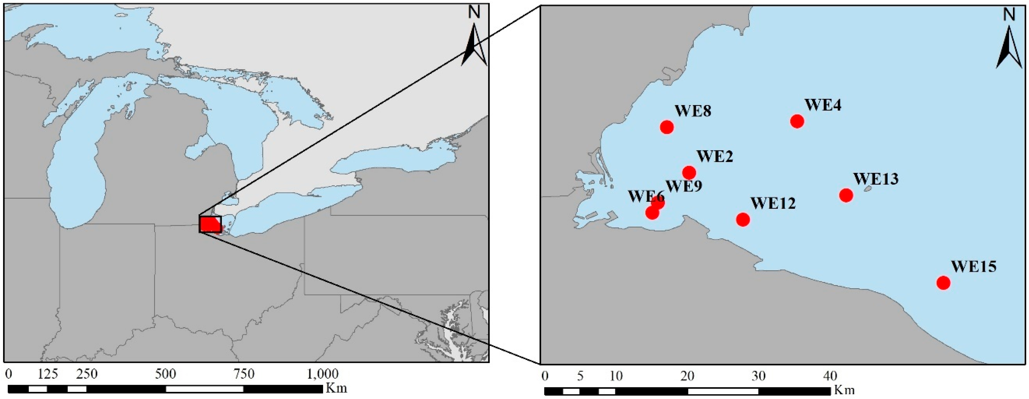
2.1. Study Site

Lake Erie is one of the Laurentian Great Lakes in North America with an average depth of 19 m. This lake can be bathymetrically separated into three distinct basins: western, central, and eastern basins. The western basin is the most turbid and shallowest, with an average depth of 7.4 m [15]. It is also the western basin which receives most of the nutrient loads and CHABs have been observed as the dominant phytoplankton group in this region since 1942 [16]. CHABs not only impair the water quality and ecosystem integrity of Lake Erie but also have the potential to produce potent toxins, generating significant public health risks and economic losses.

Recently, Lake Erie experienced high magnitude CHAB events. In 2011, the CHAB began in mid-July and covered an area of ∼600 km² [17]. In August of 2014, a CHAB caused the water supply shutdown to over 500,000 residents in Toledo, Ohio [18]. In 2015, the peak of the CHAB spread to 200 km across most of the lake [19]. These events affect Lake Erie’s water quality, which supplies more than 11 million people via its multiple uses (commercial fisheries, leisure and recreational activities, and drinking water). Therefore, the monitoring of CHABs is essential to effectively manage this important aquatic system.

2.2. Measured Pigments

PC and chl-a concentrations were measured by the Great Lakes Environmental Research Laboratory (GLERL) in collaboration with the Cooperative Institute for Great Lakes Research (CIGLR). They monitor eight stations bi-weekly in May/June and weekly from July to October (with some variance between years). In the manuscript, PC and chl-a concentration measured from water samples collected in the subsurface (0.75m) between 2016 to 2018 were used to match up with Sentinel 3/OLCI images. Figure 1 shows GLERL/CIGLR sampling locations in the Western region of Lake Erie, U.S.A. Chl-a-concentration was measured by concentrating lake water on a Glass Fiber Filter (GF/F) filter (Whatman, 47 mm). The extraction of the pigment from this filter was conducted with acetone under low light and analyzed with a 10 AU fluorometer [20]. For PC concentration measurements, concentrated lake water on a GF/F filter (Whatman, 47 mm) were extracted in phosphate buffer (Ricca Chemical, pH 6.8) using two freeze–thaw cycles, followed by sonication [21]. The extracted solution was fluorometrically measured on a Turner Aquafluor fluorometer, and fluorescence values were converted to PC concentration using a calibration curve from a series of dilutions of a commercial standard (Sigma-Aldrich).

2.3. Satellite Imagery

2.3.1. Data Acquisition

Satellite images were acquired from the Copernicus Online Data Access (REProcessed) managed by the European Organization for the Exploitation of Meteorological Satellites (EUMETSAT) [22]. Sentinel-3A OLCI Full Resolution (FR) Level-1 product and Sentinel-3A OLCI Full Resolution (FR) Level-2 water quality products were downloaded for the dates matching up the weekly samplings in Lake Erie, U.S.A. A total of 22 cloud-free images were found from 2016 to 2018 over Lake Erie. From these 22 images, 13 images were acquired on the same day of the field sampling, 5 images were acquired the day before the field sampling, and 4 images were acquired the day after the field sampling.

2.3.2. Atmospheric Correction

As described in the previous section, two types of products were downloaded: the Sentinel-3A OLCI Full Resolution (FR) Level-1 product and the Sentinel-3A OLCI Full Resolution (FR) Level-2 water quality product. The Level-2 water quality product uses an Alternative Atmospheric Correction algorithm (AAC) for the atmospheric correction. This algorithm is based on a neural network procedure which uses as inputs top-of-atmosphere reflectances (corrected for absorbing gases and smile effect) and observation geometry [23]. Through this process, it provides water-leaving reflectances and aerosol optical thickness in different wavelengths. While this Level 2 product provides an atmospheric corrected image, the Level 1 product provides the original image. To perform the atmospheric correction on the Level 1 product, the Case 2 Regional Coast-Colour (commonly known as C2RCC) was used. The C2RCC is available through the European Space Agency’s Sentinel Toolbox, and it is used to generate the Case 2 water products in Sentinel 3/OLCI. The algorithm is also based on a neural network algorithm which relies on a large database of simulated water-leaving reflectances and related top-of-atmosphere radiances [24].

2.4. Evaluation of OLCI Imagery to Retrieve PC and chl-a

2.4.1. Atmospheric Correction Comparison

To select the best product, we compared the two atmospheric correction procedures: one from the Level 1 product processed with the C2RCC algorithm and the Level 2 product processed with the AAC algorithm. Since no in situ remote sensing reflectance (R_rs) spectra were available, the comparison between these two atmospheric correction procedures was based on the spectral differences between R_rs spectra from both images. Additionally, normality and t-test were used to evaluate if the R_rs spectra were statistically different from one atmospheric correction method to another. To do that, each spectral band was compared to its respective spectral band in the other atmospherically corrected product. The t-test (t) was used when the dataset passed the normality test, and if it did not pass the normality test, a Mann–Whitney U test (U) was used.

2.4.2. Remote Sensing Algorithms Comparison

Remote sensing algorithms can be divided into different types, such as empirical, semi-empirical, semi-analytical, and quasi-analytical [25]. In this study, only semi-empirical algorithms were evaluated since semi-empirical algorithms have been commonly used to estimate PC and chl-a concentration. The most common structures of semi-empirical algorithms are two bands algorithms (2BDA), three bands algorithms (3BDA) and normalized difference algorithms (commonly named indices) [26,27]. For PC estimation, the 2BDA usually uses the R_rs at 620 nm which is related to the absorption of the PC, and the R_rs at 709 nm which is related to the scattering of particles [4,8]. The same bands are usually used for the normalized difference algorithm [28] and for the 3BDA, which also uses the R_rs at 665 nm, which is related to the absorption of chl-a [5]. For the chl-a estimations, 2BDA usually uses the R_rs at 665 nm and the R_rs at 709 nm [29] while the 3BDA adds the R_rs at 754 nm, which is related to the absorption of pure water [30]. The normalized difference algorithm for chl-a estimation uses the R_rs at 665 nm and the R_rs at 709 nm [31]. A summary of these remote sensing algorithms is presented in

Table 1. Semi-empirical algorithms for the remote estimation of phycocyanin (PC).

Pigment	Acronym	Formulation	Range of Concentration (mg/m3)	References
PC	2BDA-PC	$PC\propto \left(\frac{R_{rs}\left(709\right)}{R_{rs}\left(620\right)}\right)$	0.8–79.8	[4,8]
PC	3BDA-PC *	$PC\propto \left(R_{rs}^{-1}\left(620\right)-R_{rs}^{-1}\left(665\right)\right)·R_{rs}\left(754\right)$	N/A	[5]
PC	NDPCI	$PC\propto \left(\frac{R_{rs}\left(709\right)-R_{rs}\left(620\right)}{R_{rs}\left(709\right)+R_{rs}\left(620\right)}\right)$	45–330	[28]
Chl-a	2BDA-CL	$Chl-a\propto \left(\frac{R_{rs}\left(709\right)}{R_{rs}\left(665\right)}\right)$	4–236	[29]
Chl-a	3BDA-CL	$PC\propto \left(R_{rs}^{-1}\left(665\right)-R_{rs}^{-1}\left(709\right)\right)·R_{rs}\left(754\right)$	4–236	[29,30]
Chl-a	NDCI	$Chl-a\propto \left(\frac{R_{rs}\left(709\right)-R_{rs}\left(665\right)}{R_{rs}\left(709\right)+ R_{rs}\left(665\right)}\right)$	0.9–28.1	[31]

* Adjusted for OLCI spectral bands.

.

2.4.3. OLCI Spectral Bands and Cyanobacterial Pigments

To evaluate the use of OLCI spectral band for the estimation of PC and chl-a concentration, the relationship between each spectral band and pigments was explored using images acquired on the previous day, on the same day, and one day after the field sampling. These relationships were explored using scatter plots and linear regressions [27]. Moreover, the relationship between PC and chl-a and band ratios were explored via the use of a two-dimensional (2D) color correlation plot which was computed using a web-tool named “Interactive Correlation Environment” (ICE) [32]. ICE computes all possible spectral band ratios and analyses the relationship (via a correlation coefficient, an absolute correlation coefficient or a determination coefficient) with the pigment concentration. The best band-ratio relationship for each pigment was evaluated using scatter plots and linear regressions.

3. Results

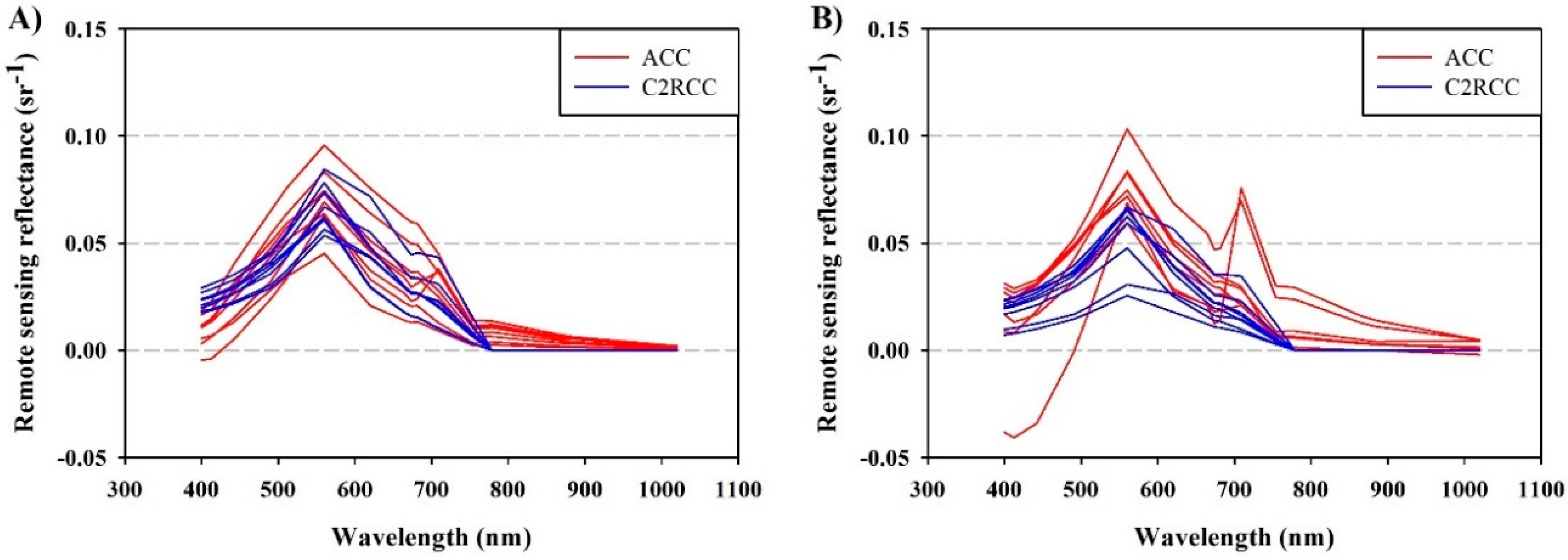
3.1. Atmospheric Correction of OLCI Images

To evaluate the best atmospheric corrected product to retrieve R_rs from an OLCI image, images from 22 August 2016 and 13 September 2016 from both atmospheric correction procedures were used. For the image from 22 August 2016, all spectral bands passed the normality test, and the t-test showed that there is a statistically significant difference between the spectral bands centered at 400 nm and 412.5 nm (P ≤ 0.001). For the other spectral bands, no statistically significant difference was found (

Table 2. Statistical differences between spectral bands from the two atmospheric correction procedures.

Image Date	Spectral Band (nm)	Normality	U or T	p-Value	Difference
08/22/2016	400	P = 0.818	−4.465	<0.001	Yes
	412.5	P = 0.652	−3.707	0.002	Yes
	442.5	P = 0.986	−1.106	0.287	No
	490	P = 0.940	0.913	0.377	No
	510	P = 0.871	1.115	0.284	No
	560	P = 0.998	0.597	0.560	No
	620	P = 0.717	0.107	0.916	No
	665	P = 0.491	0.887	0.390	No
	673.75	P = 0.461	0.969	0.349	No
	681	P = 0.437	1.030	0.321	No
	708.75	P = 0.817	1.051	0.311	No
	753.78	P = 0.859	0.441	0.666	No
09/13/2016	400	P < 0.050	20	0.620	No
	412.5	P < 0.050	24	1.000	No
	442.5	P < 0.050	19	0.535	No
	490	P < 0.050	12	0.128	No
	510	P < 0.050	10	0.073	No
	560	P = 0.659	2.790	0.016	Yes
	620	P = 0.620	1.002	0.336	No
	665	P = 0.260	1.645	0.126	No
	673.75	P = 0.890	1.370	0.196	No
	681	P = 0.747	1.511	0.157	No
	708.75	P < 0.050	7	0.026	Yes
	753.78	P < 0.050	12	0.128	No

* Shaded areas indicate where the Mann–Whitney test was applied.

). For the image from September 13, 2016; spectral bands centered at 400, 412.5, 442.5, 490, 510, 708.75, and 753.75 nm failed the normality test. The Mann–Whitney U test (U) and t-test (t) showed that only the spectral bands centered at 560 and 708.75 nm were different (Table 2).

The statistical analysis showed that both atmospheric correction algorithms have similar performance for some of the spectral bands. To select which atmospheric correction algorithm performed better, R_rs spectra were plotted (Figure 2). Figure 2A,B show that for the shorter wavelengths, the algorithms performed differently, which agrees with the statistical analysis (Table 2). Figure 2A shows that spectral features were similar while in Figure 2B, spectral features for the longer wavelengths were different (as shown in Table 2). It was observed that the image from September 13, 2016, the ACC algorithm overcorrected the R_rs for the shorter wavelengths (Figure 2B) having negative intensities. Because of these observations, the C2RCC algorithm was selected as the most appropriated for computing R_rs.

3.2. Remote Sensing Models Evaluation

Several studies evaluated remote sensing algorithms based on the simulation of OLCI spectral bands [10,11,12]. This study evaluated the performance of the most common semi-empirical algorithms.

Table 3. Statistical estimators for each algorithm for chlorophyll-a (chl-a) and PC estimation.

Algorithm	All Images (n = 164)	Day Before (n = 40)	Same Day (n = 97)	Day After (n = 27)
NDPCI	R2 = 0.011	R2 = 0.010	R2 = 0.014	R2 < 0.001
	RMSE = 69.925	RMSE = 6.265	RMSE = 88.609	RMSE = 37.127
3BDA-PC	R2 = 0.051	R2 = 0.136	R2 = 0.075	R2 < 0.001
	RMSE = 68.501	RMSE = 5.851	RMSE = 85.829	RMSE = 37.125
2BDA-PC	R2 = 0.011	R2 = 0.009	R2 = 0.015	R2 < 0.001
	RMSE = 69.922	RMSE = 6.267	RMSE = 88.597	RMSE = 37.119
NDCI	R2 = 0.003	R2 = 0.159	R2 = 0.0150	R2 = 0.002
	RMSE = 47.860	RMSE = 10.363	RMSE = 58.780	RMSE = 35.307
3BDA-CL	R2 = 0.002	R2 = 0.155	R2 = 0.013	R2 = 0.014
	RMSE = 47.882	RMSE = 10.386	RMSE = 58.842	RMSE = 35.497
2BDA-CL	R2 = 0.002	R2 = 0.163	R2 = 0.012	R2 = 0.020
	RMSE = 47.882	RMSE = 10.337	RMSE = 58.852	RMSE = 35.391

* Shaded areas indicate the best performance for each pigment.

presents the determination coefficient (R²) and the root mean square error (RMSE) for remote sensing algorithms for PC and chl-a concentration estimation from OLCI images. The performance was evaluated using all images, images collected on the same day of the field sampling, on the day before the field sampling, and during the day after the field sampling. All six selected algorithms showed poor performance for all four datasets—R² values lower than 0.2. For the dataset using all images, the range of PC concentration was 0 to 538.38 µg/L while for the chl-a concentration the range was 2.18 to 531.7 µg/L. To calculate the normalized RMSE (NRMSE) and be able to compare the RMSE for all datasets, the concentration range for each dataset was used to divide the RMSE. Therefore, the 3BDA-PC showed an NRMSE ≅ 12%, while the NDCI showed an NRMSE ≅ 9%. Other ranges of PC were 0.41 to 26.37 µg/L for the images collected on the day before the field campaign, 0 to 538.38 µg/L for the images collected on the same day of the field campaign, and 0.25 to 170.39 µg/L for the images collected the day after the field campaign. Chl-a ranges were 4.43 to 51.92 µg/L for the images collected on the day before the field campaign, 2.18 to 531.7 µg/L for the images collected on the same day of the field campaign, and 4.77 to 183.42 µg/L for the images collected the day after the field campaign. Although the values of the NRMSE showed lower percentages, because of the low R² values, it was observed that the selected remote sensing algorithms could not be used to estimate cyanobacterial pigments from OLCI images.

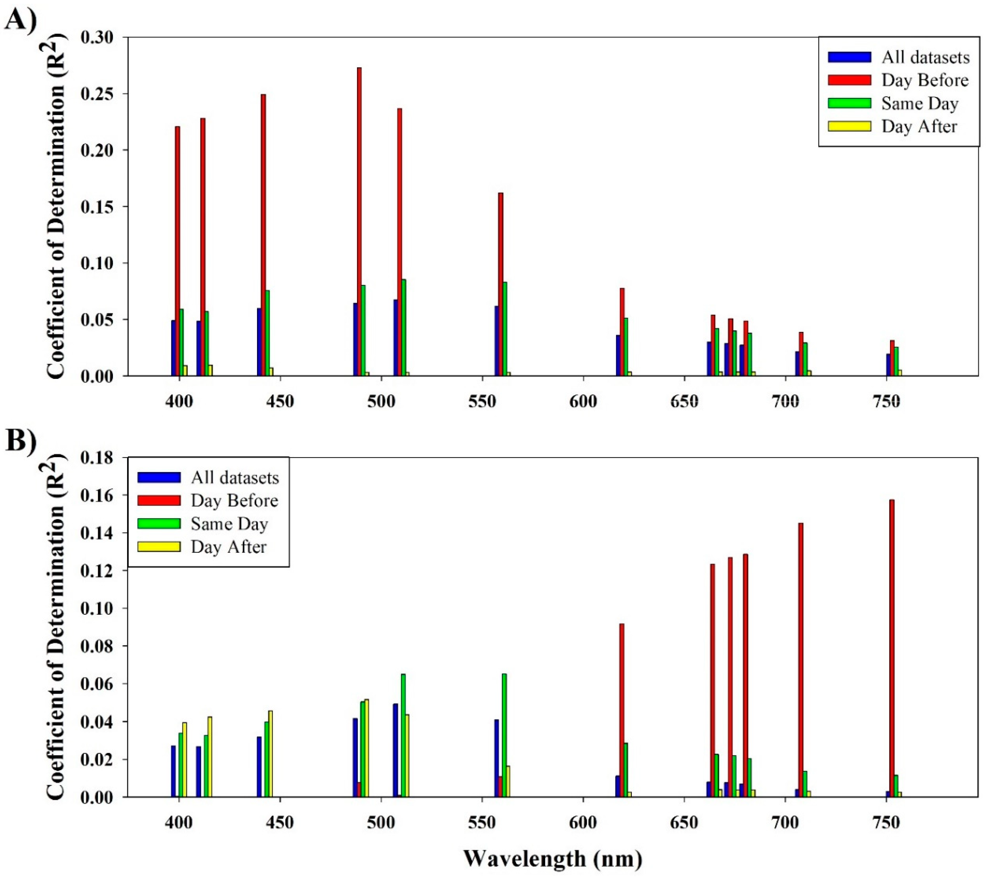
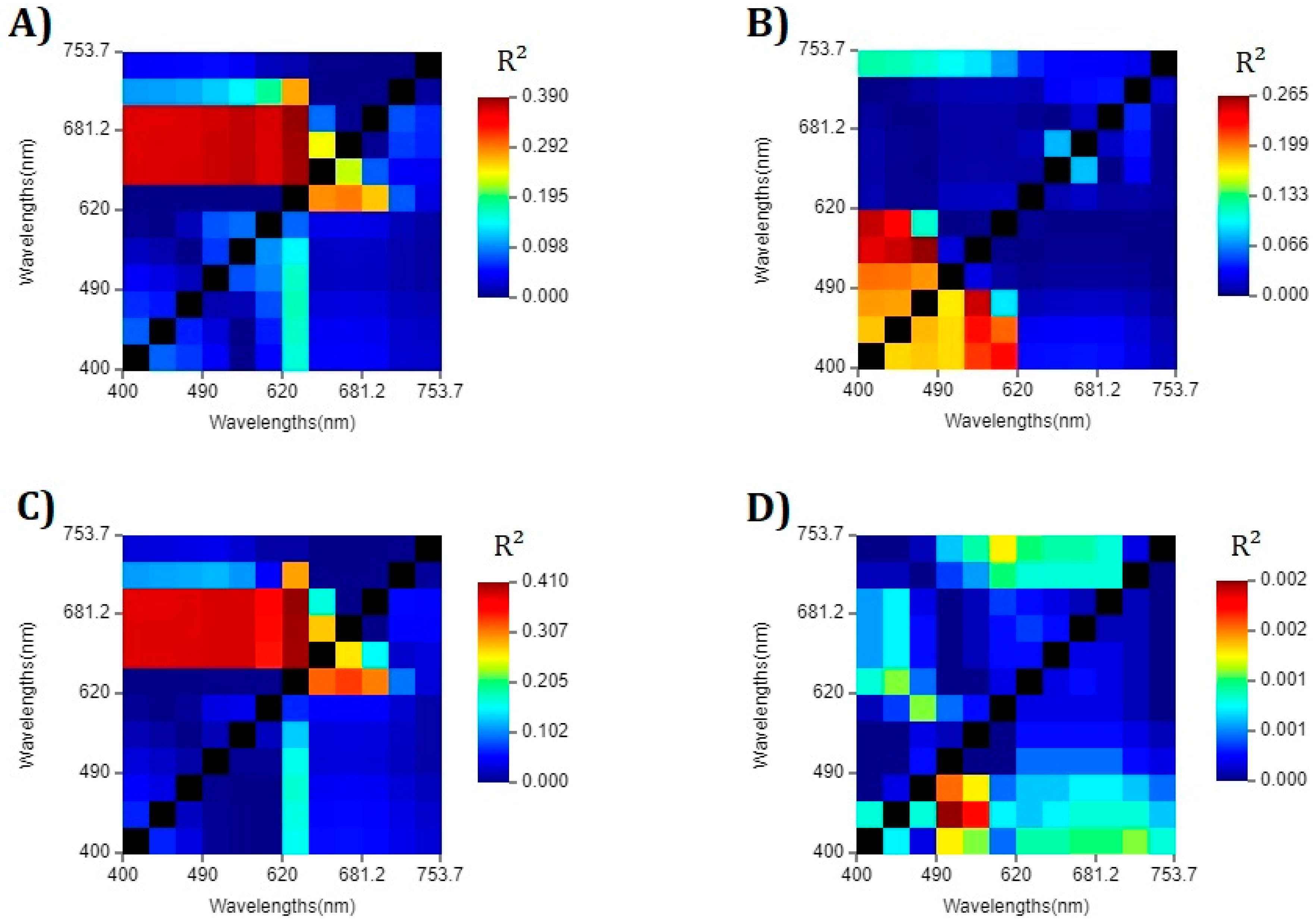
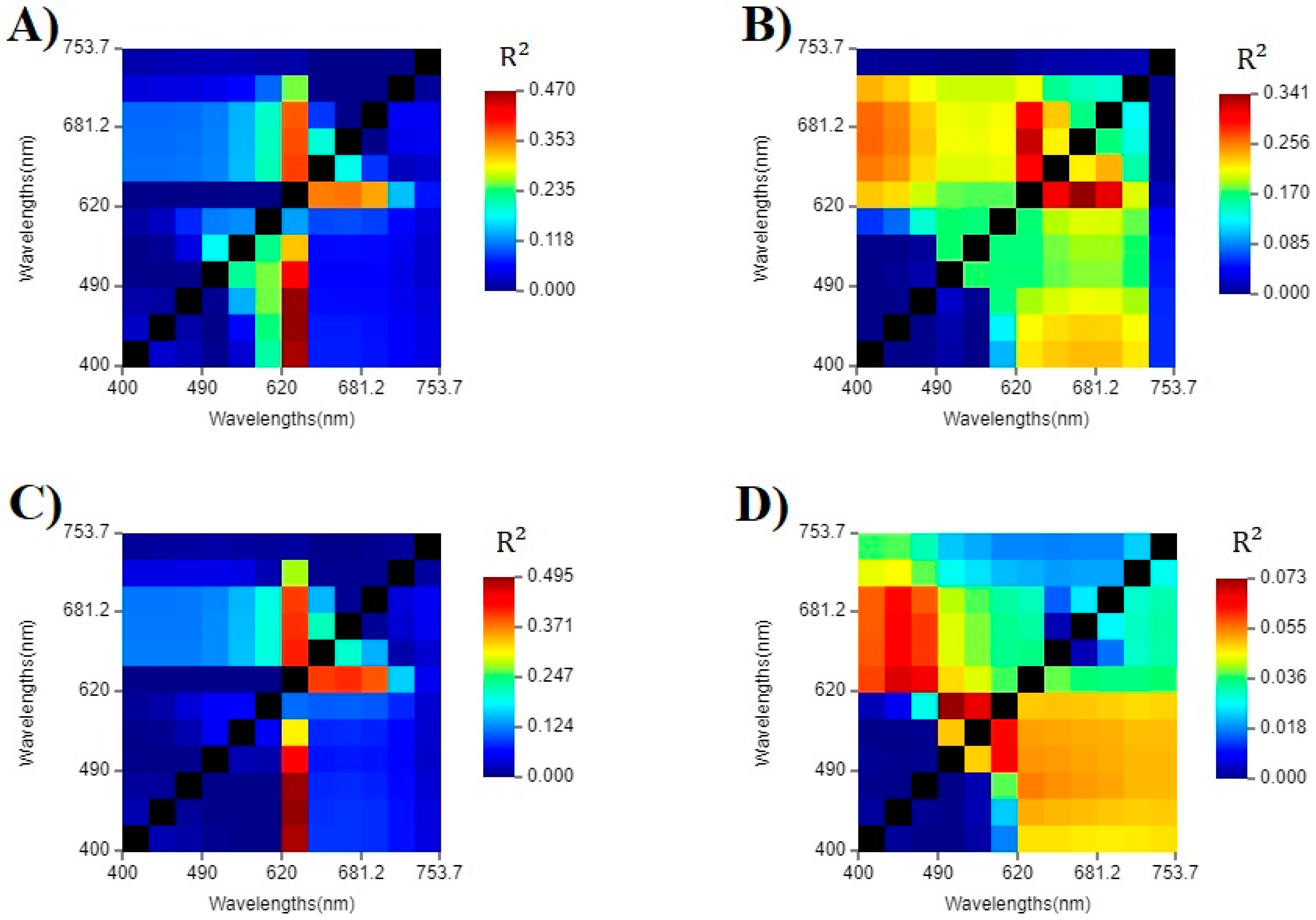
3.3. Single and Band Ratio Evaluation

Since remote sensing algorithms did not perform well, an analysis of each spectral band from OLCI was performed to evaluate the use of OLCI for the monitoring of PC and chl-a concentration. To do that, the linear relationship between each spectral band and PC and chl-a concentration were evaluated using R² values. Figure 3 presents the R² values for each spectral band for the four datasets: all images dataset, before the field campaign dataset, same day as the field campaign dataset, and the day after the field campaign dataset. Figure 3A presents the linear relationship between each spectral band and PC concentration, which is higher for the datasets of images collected before and on the same day of the field campaign for all spectral bands. Figure 3B presents the R² values for the relationship between each spectral band and chl-a concentration. For the shorter wavelengths, images from the same day of the field campaign showed higher R² values, while for longer wavelengths, images from the day before the field campaign showed higher R² values. Compared to the relationship among PC and chl-a concentration and remote sensing algorithms (Table 3), single bands resulted in a higher R² for PC estimation and a similar performance with chl-a estimations. The spectral band centered at 490 nm obtained an R² = 0.27 for the estimation of PC using images from the day before the field campaign (Figure 3) while 3BDA-PC obtained an R²=0.13 for the same dataset (Table 3). For the chl-a estimation, the spectral band centered at 753.75 nm obtained an R²= 0.15 for the estimation of chl-a using images from the day before the field campaign (Figure 3) while 2BDA-CL obtained an R²= 0.16 for the same dataset (Table 3). In addition to the improvement of R² values, the relationship between spectral bands and pigments is still weak (R² values lower than 0.3).

Band ratios among the spectral bands of OLCI in the visible and near-infrared channels were used for the computation of a 2D color correlation plot (Figure 4). This plot compares all possible band ratios from OLCI visible and near-infrared channels and relates it to PC concentrations. Figure 4A shows the best band ratio for the estimation of a PC using all images available. For this dataset, the best band ratio was the one involving the spectral bands centered at 681 and 620 nm. Figure 4B shows the best band ratio for the estimation of PC using the dataset of images collected a day before the field campaign. In this dataset, the ratio between spectral bands centered at 510 and 442.5 nm produced the highest R². Figure 4C shows the best band ratio for the estimation of PC using the dataset of images collected on the same day of the field campaign. For this dataset, the best band ratio was the same as the entire dataset (between 681 and 620 nm). Lastly, the images collected on the day after the field campaign obtained the best relationship with the ratio between 412.5 and 490 nm (Figure 4D). In comparison to remote sensing algorithms and single spectral bands, the band ratio analysis showed stronger relationships with PC concentrations. For each dataset, the use of the band ratios generated higher R² values of 0.390, 0.265, 0.410, and 0.002 for all images, for images acquired before the field campaign dataset, for images acquired on the same day as the field campaign dataset, and for images acquired on the day after the field campaign, respectively.

For chl-a estimation, the relationship with OLCI spectral band ratios was evaluated using the 2D color correlation plot in Figure 5. Figure 5A shows the best band ratio for the estimation of chl-a using all images available, which was the ratio between the spectral bands centered at 442.5 and 620 nm. This same band ratio was also the best for the dataset of images collected on the same day of the field campaign (Figure 5C). Figure 5B shows the best band ratio for the estimation of chl-a using the dataset of images collected a day before the field campaign. In this dataset, the ratio between spectral bands centered at 673.75 and 620 nm produced the highest R². Lastly, the images collected on the day after the field campaign obtained the best relationship with the ratio between 560 and 490 nm (Figure 5D). As well as the PC analysis, band ratios showed stronger relationships with chl-a concentration. For each dataset, the use of the band ratios generated higher R² values of 0.470, 0.341, 0.495, and 0.073 for all images, for images acquired before the field campaign dataset, for images acquired on the same day as the field campaign dataset, and for images acquired the day after the field campaign, respectively.

It was observed that single band (Figure 3) and band ratio (Figure 4 and Figure 5) over performed remote sensing algorithms (Table 3) on the estimation of PC and chl-a concentration.

Table 4. R² values for all tested algorithms.

Type	All Images	Day Before	Same Day	Day After
Best remote sensing algorithm (PC)	R2 = 0.051	R2 = 0.136	R2 = 0.075	R2 < 0.001
Best single band (PC)	R2 = 0.067	R2 = 0.272	R2 = 0.085	R2 = 0.009
Best band ratio (PC)	R2 = 0.390	R2 = 0.265	R2 = 0.410	R2 = 0.002
Best remote sensing algorithm (Chl-a)	R2 = 0.003	R2 = 0.163	R2 = 0.015	R2 = 0.020
Best single band (Chl-a)	R2 = 0.049	R2 = 0.157	R2 = 0.065	R2 = 0.051
Best band ratio (Chl-a)	R2 = 0.470	R2 = 0.341	R2 = 0.495	R2 = 0.073

* Shaded areas indicate the best performance for each pigment.

presents the comparison among the highest R² computed from remote sensing algorithms, single band and band ratio. The shaded areas in Table 4 indicate which method provided the highest R² value. For the estimation of PC, the band ratio using the bands centered at 681 and 620 nm obtained the highest R² values for datasets with a large range of concentration (0–538.38 µg/L). On the other hand, single bands obtained the highest R² on the datasets with lower PC concentrations (0.41–26.37 µg/L and 0.25–170.39 µg/L). For the estimation of chl-a, all datasets obtained their best performance when estimated from the identified band ratios (442.5/620; 673.75/620; and 560/490). It is important to highlight that these ratios are not common for the identification of chl-a, which usually uses the band related to the chl-a absorption (665 nm) and cells scattering (709 nm).

4. Discussion

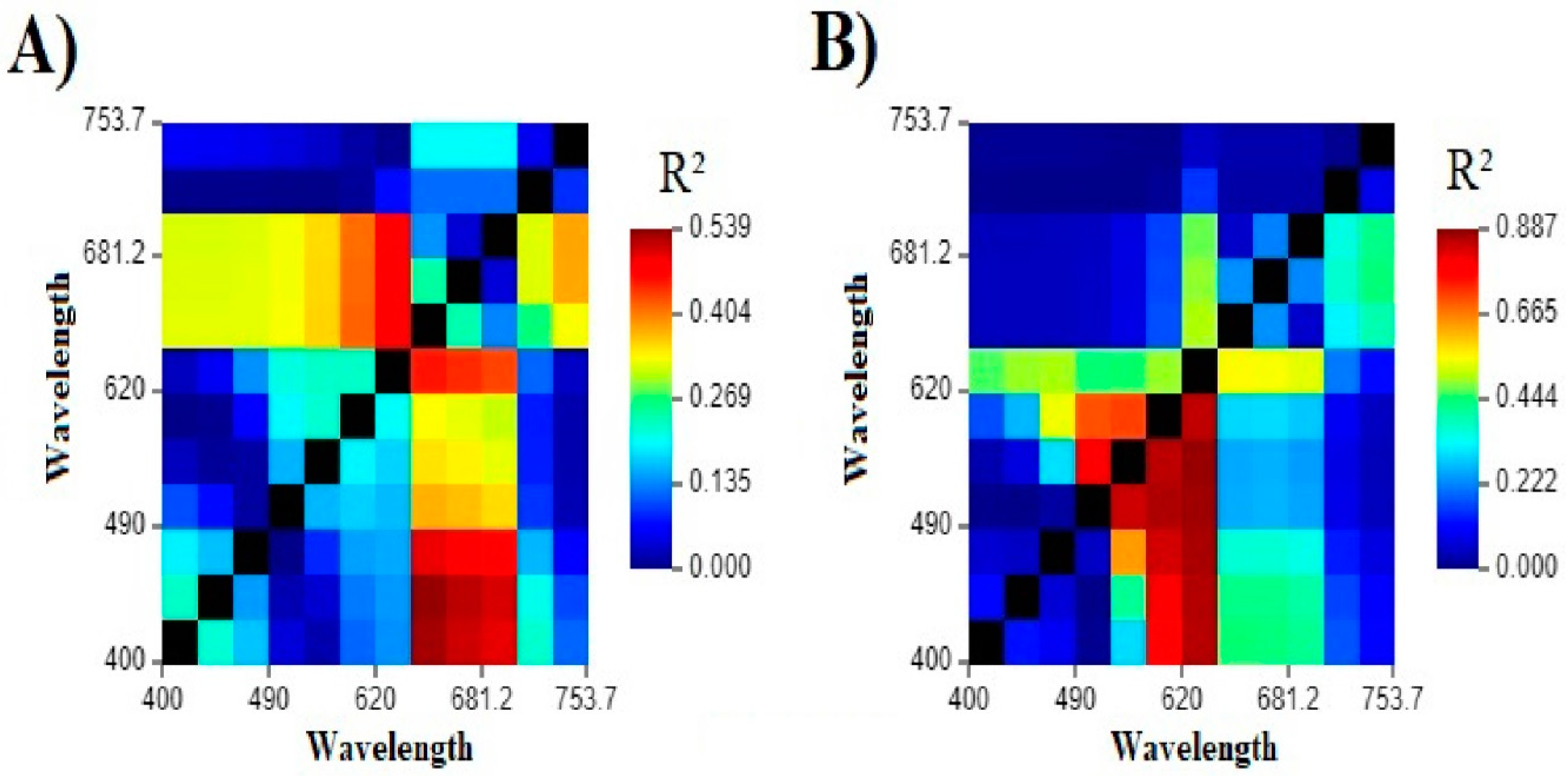
4.1. Sensitivity to Lower Concentrations

The low performances of remote sensing algorithms for both PC and chl-a estimations were surprising. However, based on the results presented in the previous section, it was observed that the lowest R² values could be related to the lower pigment concentrations. Ruiz-Verdu et al. [33] showed that for the estimation of PC, remote sensing algorithms did not perform well for PC concentrations lower than 50 µg/L. Figure 6 presents the boxplots for PC (Figure 6A) and chl-a (Figure 6B) concentrations for each dataset. It was observed that all median values for PC concentrations were lower than 10 µg/L, especially for the dates where satellite images were acquired after the field campaign (Figure 6). Therefore, the poor performance of remote sensing models could be linked to the use of datasets with most of the PC concentrations lower than 10 µg/L and chl-a lower than 50 µg/L.

To evaluate the impact of low PC and chl-a concentration, remote sensing algorithms were computed for sampling locations with concentrations higher than 50 µg/L. This threshold was based on the study by Ruiz-Verdu et al. [33] as well as in the Ohio Environmental Protection Agency (EPA) Harmful Algal Bloom Response Strategy [34]. This document classifies severe bloom by the presence of a thick scum of algal blooms over the water surface, a cyanobacteria cell count higher than 100,000 cells/mL, presence of cyanotoxins, biovolume higher than 10 mm³/L, and chl-a concentration higher than 50 μg/L. Thus, 50 µg/L is the threshold used to discriminate severe blooms, especially CHABs.

Table 5. Statistical estimators for each algorithm for chl-a and PC estimation.

Pigment	NDI	3BDA	2BDA
PC >50 µg/L (n = 8)	R2 = 0.192; RMSE = 210.432	R2 = 0.217; RMSE = 207.167	R2 = 0.185; RMSE = 211.407
Chl-a > 50 µg/L (n = 13)	R2 = 0.384; RMSE = 107.585	R2 = 0.243; RMSE = 119.201	R2 = 0.335; RMSE = 111.752

* Shaded areas indicate the best performance for each pigment.

summarizes the new estimators for the application of remote sensing models to the dataset with sampling points with high pigment concentration (>50 μg/L). The analysis was divided by the type of algorithm: normalized difference index (NDI), 3BDA, and 2BDA for each algorithm (see Table 1 for the list of algorithms). The best remote sensing algorithm for PC estimation was the 3BDA. However, the R² value was only 0.217 and the RMSE = 207.167. For the chl-a concentration, the best performance was achieved when NDI was applied with an R² = 0.384 and an RMSE= 107.858. It was also observed that R² improved when using a higher concentration of PC and chl-a, however, the RMSE and R² are not significant.

The same dataset of PC and chl-a concentrations higher than 50 µg/L was used for the computation of 2D color correlation plots for OLCI spectral bands. Figure 7 presents two 2D color correlation plots for PC estimation (Figure 7A) and for chl-a estimation (Figure 7B) higher than 50 µg/L. Similar to the results from remote sensing algorithms, band ratios showed an improvement in the relationship with higher concentrations. The relationship between PC and OLCI band ratios improved from R² = 0.410 for the same day dataset (Figure 4) to an R² = 0.539 for the dataset of PC concentrations higher than 50 µg/L. The relationship with chl-a was also improved in the dataset for pigment concentrations higher than 50 µg/L. Figure 7B shows that the band ratio between the spectral bands centered at 560 and 620 nm obtained an R² = 0.887 which is higher than the R² = 0.495 from the same day dataset (Figure 5). However, it is important to highlight that these datasets of PC and chl-a higher than 50 µg/L only have a low number of samples (8 for PC and 13 for chl-a). Therefore, these results may not well represent the relationship between band ratios and pigments, especially when there are large variations in the concentration where concentrations can vary from 50 to more than 500 µg/L (Figure 6). Nevertheless, these results corroborate with the previous results suggesting that current algorithms are not able to accurately estimate cyanobacteria pigments from OLCI.

4.2. Band Selection for the Development of Algorithms

Previous results suggest that the development of new remote sensing algorithms is needed for the estimation of PC and chl-a using OLCI. While traditional remote sensing algorithms for PC and chl-a use R_rs spectral features, such as the trough around 620 nm, the trough at 665 nm, and the peak near 700 nm (see Table 1 for algorithms), this study showed that other spectral bands may be used to estimate cyanobacteria pigments from OLCI. For PC monitoring, most of the algorithms use the R_rs around 620 nm which is primarily associated with PC absorption [4,5,6,7,8,9] and the R_rs around 709 nm which is generated by the absorption by pure water in the near infrared and the absorption of chl-a around 665 nm [35]. Some studies also use the R_rs around 650 nm, which is related to the fluorescence of PC [36]. The spectral band centered at 681 nm was only used in the spectral shape algorithm [37], which will be changed to cyanobacterial index [38]. The authors explained that at 681 nm, the presence of cyanobacteria would create a negative spectral shape because of the cyanobacteria, which overwhelms the fluorescence signal. The spectral shape algorithm (or cyanobacteria index) was developed for MERIS images over Lake Erie, U.S.A., and it is currently being applied in the Lake Erie HAB Bulletin [39]. For chl-a remote sensing algorithms other than the already mentioned spectral bands, it is common to have a spectral band centered around 753 nm, which is related to the absorption of pure water [30].

The results from the presented study indicate that Sentinel 3/OLCI could be used to monitor cyanobacteria pigments, however, traditional remote sensing algorithms should be re-formulated. For PC concentration estimation, it is suggested to use spectral bands centered at 681 and 620 nm. Figure 4A,C showed that for datasets with a higher range of PC concentration, the reflectance at 620 nm is strongly correlated to the reflectance at longer wavelengths. This is explained by the spectral features of PC which are usually related to longer wavelengths, such as the fluorescence at 650 nm and cell’s scattering at 709 nm, as well as chl-a absorption around 665 nm and chl-a fluorescence around 681 nm. For chl-a concentration estimation, it is suggested to use spectral bands centered at 442.5 and 620 nm. The R_rs around 442.5 nm is commonly used for chl-a estimation in ocean waters, and it is primarily related to the chl-a absorption [40]; however, the use of the band centered at 620 nm to estimate chl-a is uncommon, since it is related to the absorption of PC. Figure 5A,C showed that at 620 nm, the reflectance was strongly correlated to shorter wavelengths and slightly weaker correlations to longer wavelengths. Based on these results, a re-evaluation of spectral band selection for remote sensing algorithm is needed for Lake Erie, U.S.A., and it could be needed for other aquatic systems as well. Thus, this analysis has highlighted the need to re-evaluate the use of traditional algorithms on OLCI images.

Additionally, the use of the spectral band around 681 nm for PC estimation in Lake Erie could be related to an empirical factor, which could explain the fact that the spectral shape algorithm (or cyanobacteria index) did not perform well in other study sites [12]. Thus, this spectral feature around 681 nm should be explored in further studies, especially in Lake Erie. Thus, future works should focus on the bio-optical characterization of Lake Erie waters, to fully understand the dependence of the use of the band around 681 nm for the estimation of PC.

5. Conclusions

The analysis presented in this study showed that traditional remote sensing algorithms for PC and chl-a estimation did not perform well on Sentinel 3/OLCI images over Lake Erie, U.S.A. Although in this study, only images of Lake Erie were analyzed, these findings could be used as a guide for other aquatic systems. The same way that traditional remote sensing algorithms were not able to retrieve PC and chl-a information from Lake Erie, they could show the same poor performances in other environments. Based on these results, the importance of an evaluation of remote sensing algorithms using real satellite images not only using proximal remote sensing. Nevertheless, the evaluation of single bands and band ratios showed a stronger relationship (higher R² values, Table 4) to PC and chl-a concentration when compared to traditional remote sensing algorithms. This indicates that for the monitoring of CHABs in Lake Erie, it is important to develop new remote sensing algorithms and/or change the selection of spectral bands in the existing algorithms.

The analysis of single and band ratios related to PC and chl-a concentration showed that instead of the spectral band centered at approximately 709 nm, remote sensing algorithms use the spectral band centered at 681 nm for the estimation of PC concentration. For chl-a concentration, the spectral bands that showed a stronger relationship to chl-a were 442.5 nm and 620 nm. Based on these findings, the importance of collecting accurate and precise in situ radiometric data is highlighted. Moreover, it is important to emphasize that in situ hyperspectral R_rs data from Lake Erie is essential for the development of new tools. Therefore, future work should focus on a large field campaign of radiometric data in Lake Erie, especially during the CHABs season.

References

1. Palmer, S.C.; Kutser, T.; Hunter, P.D. Remote sensing of inland waters: Challenges, progress and future directions. Remote. Sens. Environ. 2015, 157, 1–8. [Google Scholar] [CrossRef] [Green Version]
2. Donlon, C.; Berruti, B.; Buongiorno, A.; Ferreira, M.-H.; Féménias, P.; Frerick, J.; Goryl, P.; Klein, U.; Laur, H.; Mavrocordatos, C.; et al. The Global Monitoring for Environment and Security (GMES) Sentinel-3 mission. Remote. Sens. Environ. 2012, 120, 37–57. [Google Scholar] [CrossRef]
3. Reinart, A.; Kutser, T. Comparison of different satellite sensors in detecting cyanobacterial bloom events in the Baltic Sea. Remote. Sens. Environ. 2006, 102, 74–85. [Google Scholar] [CrossRef]
4. Ogashawara, I.; Mishra, D.R.; Mishra, S.; Curtarelli, M.P.; Stech, J.L. A Performance Review of Reflectance Based Algorithms for Predicting Phycocyanin Concentrations in Inland Waters. Remote. Sens. 2013, 5, 4774–4798. [Google Scholar] [CrossRef] [Green Version]
5. Hunter, P.; Tyler, A.; Presing, M.; Kovacs, A.; Preston, T. Spectral discrimination of phytoplankton colour groups: The effect of suspended particulate matter and sensor spectral resolution. Remote. Sens. Environ. 2008, 112, 1527–1544. [Google Scholar] [CrossRef]
6. Dekker, A.G. Detection of Optical Water Quality Parameters for Eutrophic Waters by High Resolution Remote Sensing. Ph.D. Thesis, Vrije Universiteit, Amsterdam, The Netherlands, 1993. [Google Scholar]
7. Vincent, R.K.; Qin, X.; McKay, R.L.; Miner, J.; Czajkowski, K.; Savino, J.; Bridgeman, T. Phycocyanin detection from LANDSAT TM data for mapping cyanobacterial blooms in Lake Erie. Remote. Sens. Environ. 2004, 89, 381–392. [Google Scholar] [CrossRef]
8. Simis, S.G.H.; Peters, S.W.M.; Gons, H.J. Remote sensing of the cyanobacterial pigment phycocyanin in turbid inland water. Limnol. Oceanogr. 2005, 50, 237–245. [Google Scholar] [CrossRef]
9. Li, L.; Sengpiel, R.E.; Pascual, D.L.; Tedesco, L.P.; Wilson, J.S.; Soyeux, E. Using hyperspectral remote sensing to estimate chlorophyll-aand phycocyanin in a mesotrophic reservoir. Int. J. Sens. 2010, 31, 4147–4162. [Google Scholar] [CrossRef]
10. Lunetta, R.S.; Schaeffer, B.A.; Stumpf, R.P.; Keith, D.; Jacobs, S.A.; Murphy, M.S. Evaluation of cyanobacteria cell count detection derived from MERIS imagery across the eastern USA. Remote. Sens. Environ. 2015, 157, 24–34. [Google Scholar] [CrossRef]
11. Woźniak, M.; Bradtke, K.M.; Darecki, M.; Krężel, A. Empirical Model for Phycocyanin Concentration Estimation as an Indicator of Cyanobacterial Bloom in the Optically Complex Coastal Waters of the Baltic Sea. Remote. Sens. 2016, 8, 212. [Google Scholar] [CrossRef]
12. Beck, R.; Xu, M.; Zhan, S.; Liu, H.; Johansen, R.A.; Tong, S.; Yang, B.; Shu, S.; Wu, Q.; Wang, S.; et al. Comparison of satellite reflectance algorithms for estimating phycocyanin values and cyanobacterial total biovolume in a temperate reservoir using coincident hyperspectral aircraft imagery and dense coincident surface observations. Remote. Sens. 2017, 9, 538. [Google Scholar] [CrossRef]
13. Mishra, D.R.; Mishra, S. A novel remote sensing algorithm to quantify phycocyanin in cyanobacterial algal blooms. Environ. Lett. 2014, 9, 114003. [Google Scholar] [CrossRef]
14. Liu, G.; Simis, S.G.H.; Li, L.; Wang, Q.; Li, Y.; Song, K.; Lyu, H.; Zheng, Z.; Shi, K. A four-band semi-analytical model for estimating phycocyanin in inland waters from simulated MERIS and OLCI data. IEEE T. Geosci. Remote Sens. 2017, 56, 1374–1385. [Google Scholar] [CrossRef]
15. Lake Erie LaMP. Lake Erie Binational Nutrient Management Strategy: Protecting Lake Erie by Managing Phosphorus. Available online: https://www.epa.gov/sites/production/files/2015-10/documents/binational_nutrient_management.pdf (accessed on 02 March 2019).
16. Allinger, L.E.; Reavie, E.D. The ecological history of Lake Erie as recorded by the phytoplankton community. J. Great Lakes 2013, 39, 365–382. [Google Scholar] [CrossRef]
17. Michalak, A.M.; Anderson, E.J.; Beletsky, D.; Boland, S.; Bosch, N.S.; Bridgeman, T.B.; Chaffin, J.D.; Cho, K.; Confesor, R.; Daloğlu, I.; et al. Record-setting algal bloom in Lake Erie caused by agricultural and meteorological trends consistent with expected future conditions. Proc. Natl. Acad. Sci. USA 2013, 110, 6448–6452. [Google Scholar] [CrossRef] [PubMed] [Green Version]
18. Paerl, H.W.; Gardner, W.S.; McCarthy, M.J.; Peierls, B.L.; Wilhelm, S.W. Algal blooms: Noteworthy nitrogen. Science 2014, 346, 175. [Google Scholar] [CrossRef]
19. Michalak, A.M. Study role of climate change in extreme threats to water quality. Nature 2016, 535, 349–350. [Google Scholar] [CrossRef]
20. Speziale, B.J.; Schreiner, S.P.; Giammatteo, P.A.; Schindler, J.E. Comparison of N,N-Dimethylformamide, Dimethyl Sulfoxide, and Acetone for Extraction of Phytoplankton Chlorophyll. Can. J. Fish. Aquat. Sci. 1984, 41, 1519–1522. [Google Scholar] [CrossRef]
21. Horváth, H.; Kovacs, A.W.; Riddick, C.; Présing, M. Extraction methods for phycocyanin determination in freshwater filamentous cyanobacteria and their application in a shallow lake. Eur. J. Phycol. 2013, 48, 278–286. [Google Scholar] [CrossRef] [Green Version]
22. Copernicus Online Data Access. Available online: https://coda.eumetsat.int/#/home (accessed on 2 March 2019).
23. Alternative Atmospheric Correction (Neural Network). Available online: https://sentinel.esa.int/web/sentinel/technical-guides/sentinel-3-olci/level-2/alternative-atmospheric-correction (accessed on 2 March 2019).
24. Brockmann, C.; Doerffer, R.; Peters, M.; Kerstin, S.; Embacher, S.; Ruescas, A. Evolution of the C2RCC neural network for Sentinel 2 and 3 for the retrieval of ocean colour products in normal and extreme optically complex waters. In Proceedings of the Living Planet Symposium 2016, Prague, Czech Republic, 9–13 May 2016. [Google Scholar]
25. Ogashawara, I. Terminology and classification of bio-optical algorithms. Sens. Lett. 2015, 6, 613–617. [Google Scholar] [CrossRef]
26. Beck, R.; Zhan, S.; Liu, H.; Tong, S.; Yang, B.; Xu, M.; Ye, Z.; Huang, Y.; Shu, S.; Wu, Q.; et al. Comparison of satellite reflectance algorithms for estimating chlorophyll-a in a temperate reservoir using coincident hyperspectral aircraft imagery and dense coincident surface observations. Remote. Sens. Environ. 2016, 178, 15–30. [Google Scholar] [CrossRef] [Green Version]
27. Augusto-Silva, P.B.; Ogashawara, I.; Barbosa, C.C.F.; De Carvalho, L.A.S.; Jorge, D.S.F.; Fornari, C.I.; Stech, J.L. Analysis of MERIS reflectance algorithms for estimating chlorophyll-a concentration in a Brazilian reservoir. Remote. Sens. 2014, 6, 11689–11707. [Google Scholar] [CrossRef]
28. Gómez, J.A.D.; Alonso, C.A.; García, A.A. Remote sensing as a tool for monitoring water quality parameters for Mediterranean Lakes of European Union water framework directive (WFD) and as a system of surveillance of cyanobacterial harmful algae blooms (SCyanoHABs). Environ. Monit. Assess. 2011, 181, 317–334. [Google Scholar] [CrossRef] [PubMed]
29. Dall’Olmo, G.; Gitelson, A.A.; Dall’Olmo, G. Effect of bio-optical parameter variability on the remote estimation of chlorophyll-a concentration in turbid productive waters: experimental results. Appl. Opt. 2005, 44, 412. [Google Scholar] [CrossRef] [PubMed]
30. Gitelson, A.A.; Gritz, Y.; Merzlyak, M.N. Relationships between leaf chlorophyll content and spectral reflectance and algorithms for non-destructive chlorophyll assessment in higher plant leaves. J. Plant Physiol. 2003, 160, 271–282. [Google Scholar] [CrossRef] [PubMed]
31. Mishra, S.; Mishra, D.R. Normalized difference chlorophyll index: A novel model for remote estimation of chlorophyll-a concentration in turbid productive waters. Remote. Sens. Environ. 2012, 117, 394–406. [Google Scholar] [CrossRef]
32. Ogashawara, I.; Curtarelli, M.P.; Souza, A.F.; Augusto-Silva, P.B.; Alcântara, E.H.; Stech, J.L. Interactive Correlation Environment (ICE)—A statistical web tool for data collinearity analysis. Remote. Sens. 2014, 6, 3059–3074. [Google Scholar] [CrossRef]
33. Ruiz-Verdú, A.; Simis, S.G.; De Hoyos, C.; Gons, H.J.; Peña-Martinez, R. An evaluation of algorithms for the remote sensing of cyanobacterial biomass. Remote. Sens. Environ. 2008, 112, 3996–4008. [Google Scholar] [CrossRef]
34. Ohio Environmental Protection Agency. Public Water System Harmful Algal Bloom Response Strategy. Available online: http://epa.ohio.gov/Portals/28/documents/habs/PWS_HAB_Response_Strategy.pdf (accessed on 2 March 2019).
35. Gitelson, A. The peak near 700 nm on radiance spectra of algae and water: relationships of its magnitude and position with chlorophyll concentration. Int. J. Sens. 1992, 13, 3367–3373. [Google Scholar] [CrossRef]
36. Schalles, J.F.; Yacobi, Y.Z. Remote detection and seasonal patterns of phycocyanin, carotenoid, and chlorophyll pigments in eutrophic waters. Arch. Hydrobiol. 2000, 55, 153–168. [Google Scholar]
37. Wynne, T.T.; Stumpf, R.P.; Tomlinson, M.C.; Warner, R.A.; Tester, P.A.; Dyble, J.; Fahnenstiel, G.L. Relating spectral shape to cyanobacterial blooms in the Laurentian Great Lakes. Int. J. Sens. 2008, 29, 3665–3672. [Google Scholar] [CrossRef]
38. Wynne, T.T.; Tomlinson, M.C.; Stumpf, R.P.; Dyble, J. Characterizing a cyanobacterial bloom in Western Lake Erie using satellite imagery and meteorological data. Limnol. Oceanogr. 2010, 55, 2025–2036. [Google Scholar] [CrossRef] [Green Version]
39. Lake Erie HAB Bulletin. Available online: https://www.glerl.noaa.gov/res/HABs_and_Hypoxia/lakeErieHABArchive/ (accessed on 2 March 2019).
40. Claustre, H.; Bricaud, A.; Babin, M.; Morel, A. Variability in the chlorophyll-specific absorption coefficients of natural phytoplankton: Analysis and parameterization. J. Geophys. Res. Biogeosci. 1995, 100, 13321. [Google Scholar]
Figure 1. Sampling locations from the Great Lakes Environmental Research Laboratory/Cooperative Institute for Great Lakes Research (GLERL/CIGLR) at the Western region of Lake Erie, U.S.A.
Environments 06 00060 g001
Figure 2. Rrs spectra extracted from sampling points from GLERL in the Western region of Lake Erie, U.S.A. (A) Rrs spectra from 22 August 2016 image; (B) Rrs spectra from 13 September 2016 image.
Environments 06 00060 g002
Figure 3. Determination coefficient (R2) values for a linear relationship between each OLCI’ spectral band and (A) Phycocyanin (PC) concentrations and (B) Chlorophyll-a (Chl-a) concentration.
Environments 06 00060 g003
Figure 4. 2D color R2 plots for PC concentration estimation (A) R2 values for all data; (B) R2 values for the day before the field sampling data; (C) R2 values for same day of the field sampling data, and (D) R2 values for the day after the field sampling data.
Environments 06 00060 g004
Figure 5. 2D color R2 plots for chl-a concentration estimation (A) R2 values for all data; (B) R2 values for the day before the field sampling data; (C) R2 values for same day of the field sampling data, and (D) R2 values for the day after the field sampling data.
Environments 06 00060 g005
Figure 6. Boxplots for PC and chl-a concentration for each dataset (A) For PC concentration; (B) For chl-a concentration.
Environments 06 00060 g006
Figure 7. 2D color R2 plots higher concentrations (>50 µg/L) (A) For PC concentration; (B) For chl-a concentration.
Environments 06 00060 g007