Fractal and Long-Memory Traces in PM₁₀ Time Series in Athens, Greece

Abstract

This work examines if chaos and long memory exist in PM₁₀ concentrations recorded in Athens, Greece. The algorithms of Katz, Higuchi, and Sevcik were employed for the calculation of fractal dimensions and Rescaled Range (R/S) analysis for the calculation of the Hurst exponent. Windows of approximately two months’ duration were employed, sliding one sample forward until the end of each utilized signal. Analysis was applied to three long PM₁₀ time series recorded by three different stations located around Athens. Analysis identified numerous dynamical complex fractal time-series segments with patterns of long memory. All these windows exhibited Hurst exponents above 0.8 and fractal dimensions below 1.5 for the Katz and Higuchi algorithms, and 1.2 for the Sevcik algorithm. The paper discusses the importance of threshold values for the postanalysis of the discrimination of fractal and long-memory windows. After setting thresholds, computational calculations were performed on all possible combinations of two or more techniques for the data of all or two stations under study. When all techniques were combined, several common dates were found for the data of the two combinations of two stations. When the three techniques were combined, more common dates were found if the Katz algorithm was not included in the meta-analysis. Excluding Katz’s algorithm, 12 common dates were found for the data from all stations. This is the first time that the results from sliding-window chaos and long-memory techniques in PM₁₀ time series were combined in this manner.

1. Introduction

Urban air pollution is a problem related to a sustainable environment, and human society and economy [1,2]. Caused by human intervention, urban air pollution is now a sustained ever-changing part of the urban environment, governed by mechanisms such as emission, dilution, and transportation [3]. Significant pollutants are sulphur dioxides and nitrogen oxides, the ozone, and respirable particulate matter (PM) [4]. The scientific research of the topic focuses on understanding the variations of urban air pollutants with respect to time, investigating the contribution of environmental and meteorological parameters to those variations through modeling, forecasting, and predicting future trends and alterations. Noteworthy approaches utilize neural networks [5,6,7,8,9,10,11,12,13,14,15,16], wavelets [17,18], statistical [19,20], and deterministic [21] models, and, currently, cutting-edge techniques based on chaos and complexity (e.g., References [4,22,23,24,25,26,27,28,29,30,31,32,33,34,35,36]). Since no forecast method is solid, reliable, and accurate enough to sufficiently match all air-contamination time series [37], it is a challenging task to achieve credible estimations. Their main limitations are related to a lack in measurements, gaps in knowledge on the interaction of air pollutants with the atmosphere, and the fact that it is not fully understood if urban air-pollution variations are governed by randomness or dynamical complexity. The exploration of the latter topic has recently gained particular attention.

The science of complex dynamical systems involves diverging techniques for the investigation of interstate transitions of such systems. Techniques based on fractals [38,39,40,41,42,43,44,45,46] and long-memory [41,43,44,45,47] receive particular interest because they succeed in delineating the hidden traces of the time series of numerous physical systems of different types, importantly: stationary, nonstationary, and irregular [48,49]. Regarding air-pollution environmental systems, Shi et al. [24] reported two power laws in three air-pollution time series in Shanghai, China, indicating different self-organised critical (SOC) states. Liu et al. [4] employed detrended fluctuation analysis (DFA) and multifractals to investigate the temporal variations of SO₂, NO₂, and PM₁₀ concentrations in the city of Shanghai, China. They reported that the corresponding air pollution was a self-organised critical (SOC) process. They observed different SOC behaviour within the SO₂, NO₂, and PM₁₀ concentration time series that were attributed to differences in corresponding power-law relations. Varotsos et al. [31] observed power-law correlations and the persistent behaviour of deseasonalised ozone-concentration time series with lags between one week and five years. Lee et al. [50] reported scaling invariance and decreasing box-dimension function in the hourly average of O₃ time series concentrations during a whole year by analysing their data series with monofractals. Windsor and Toumi [35] reported, through R/S analysis, a high persistency of an hourly ozone-concentration time series extending up to 400 days. Similarly, Weng et al. [34] confirmed, through R/S analysis, the nonlinearity, fractality, persistency, and long-lasting characteristics of deseasonalised ground-level peak ozone-concentration time series in southern Taiwan. Xue at al. [51] concluded that R/S analysis, DFA, power-law spectral analysis, linear unbiased estimates, correlation analyses, and power-spectrum analysis are sophisticated approaches to analyse and describe the distribution, periodicity, and trends of air-pollutant concentrations. Similarly, Dong et al. [52] employed DFA and multifractal DFA in PM_2.5 and PM₁₀ data series, and reported the statistical self-affinity, long-memory, and multifractality of their pollutant time series. Finally, Yuval and broday [33] employed continuous wavelet-transform fractal analysis and found that the predictability of air pollutants is consistent with that of meteorological variables in the short scale.

2. Experimental Methods

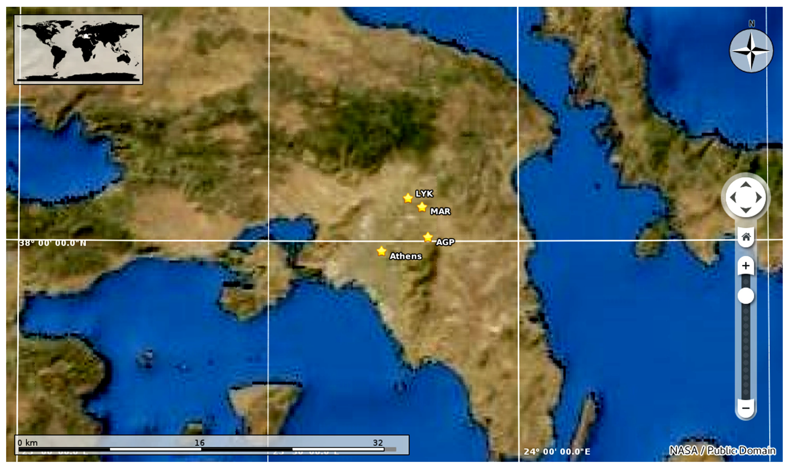
2.1. Area of Study

Athens is an urban area with approximately four million habitants and air-contamination issues similar to other large cities worldwide [53]. The city of Athens is situated in a zone of complex geography inside the Athens basin (approximately 450 km²). Mountains frame the city on the west, north and east, with heights ranging from 400 up to 1500 m (Figure 1). Openings between these mountains are found northeast and west of the basin, while the ocean broadens southward (Saronikos Gulf). The major axis of the Athens basin is from the southwest to the northeast. Usually, winds in the Athens basin blow from the north and northeast in the late summer, fall, and winter, but from the south–southwest in spring and late spring. The northeastern and southwestern directions coincide with the major geographical axis of the basin. During the prevalence of local circulation systems, the basin’s ventilation is poor [54,55]. Generally, the dispersion of air pollutants is not favoured by the topography. Air-pollutant emissions in Athens are mainly due to vehicles, industry, and domestic heating.

2.2. Measurement Methodology

PM₁₀ data were retrieved by the Department of Environmental Protection of the Hellenic Ministry of Environment and Energy. This department constantly monitors pollutant concentrations throughout each day. The automatic analysers employed in the measurements provide data every minute. From these data, daily average-pollution time series are calculated via microprocessors, located inside each automatic analyser. All values are transferred to the central station where they are further processed and stored. The present paper uses the daily PM₁₀ time series collected between 2001 and 2016 from the Agia Paraskevi (AGP), Maroussi (MAR) and Lykovrissi (LYK) stations (Figure 1). PM₁₀ detection is conducted via beta radiation absorption.

3. Chaos Analysis Methods

3.1. Fractality and Long-Memory

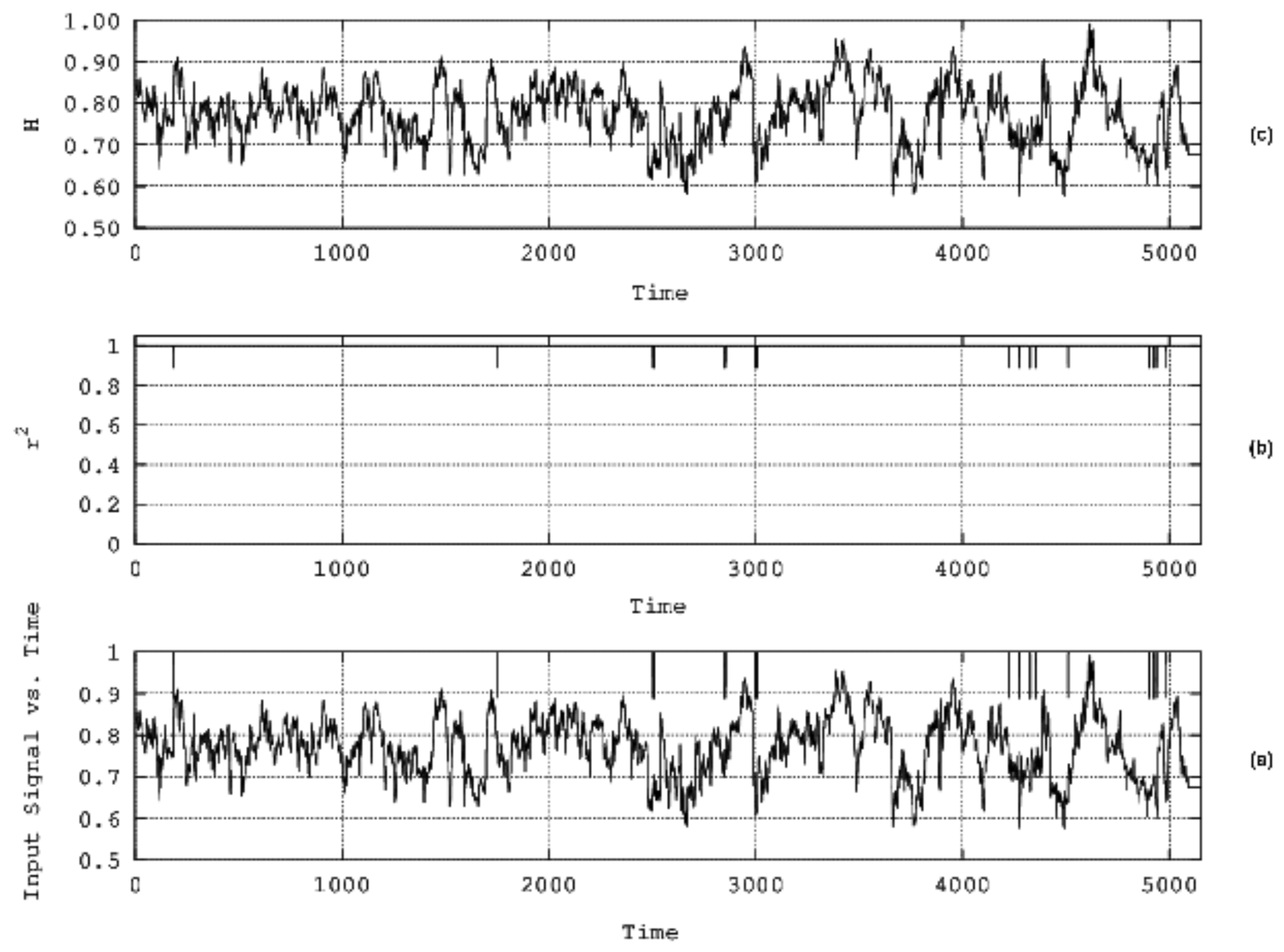
Nature exhibits fractal behaviour in several physical systems that reflect this when dilated, translated, or rotated in space. Depending on their mathematical properties, these systems are characterised as self-affine or self-similar. Such systems are fractals because the self-affinity and the self-similarity characterise all parts of the system in a manner that every part is a large or small scale imitation or representation of the whole system. Due to this property, fractal systems can be investigated by analysing their parts. It is notable that scaling and fractal behaviour are associated with a system’s long-memory [56,57,58] and complexity [57], where the complexity of a system indicates the existence of linear mechanisms and orderliness [59,60]. The complexity, fractality, and long memory of a system are closely related. For this reason, long-memory analysis can reveal the fractality and the complexity of a system [43,44,45,61]. The long-memory analysis of a system can show if there are strong associations between the past, present, and future states of the system.

Among the various methods for estimating the fractality of a system, the ones that directly calculate the fractal dimension are advantageous. These methods reveal the long memory of the system as well. A direct method for estimating the long memory of a system is R/S analysis [41,45,46,47,62,63,64].

In the following, these methods are described in detail. As associated with the calculations, the Hurst exponent [62] is analysed first since all the methods in the following are combined in terms of Hurst exponents.

3.2. Hurst Exponent

Hurst exponent (H) is a parameter that can reveal patterns of long memory hidden in time series, namely, long-lasting associations in time or space [41,45,46,47,62,63,64]. It can be used to assess if the relevant phenomenon is a time-evolving fractal, and the associated time series is smooth [65]. The Hurst exponent has been employed in different research topics, e.g., in hydrological [62,63] and astrophysical applications [66], the physics of plasma turbulence [67], capital-markets processes [68], noisy observations of traffic traces [69], pre-earthquacke time series [39,43,44,45,64,70,71,72,73,74], seizures prior to epilepsy [75], and climate dynamics [76].

The value range of the Hurst exponent is indicative of the following issues [39,43,44,45,62,63,64,70,71,72,73,74]:

(i)

If 0.5 < H < 1, there is a positive long-range autocorrelation in the associated time series. If so, high present values are followed, most probably, by high future values, while the trend continues long into the future (persistency);

(ii)

if 0 < H < 0.5, there are long-lasting changes between low and high values. When this happens, low present values are followed by high future values, and vice versa. This low–high value change continues long into the future of the time series (antipersistency);

(iii)

if H = 0.5, the time series is random and uncorrelated.

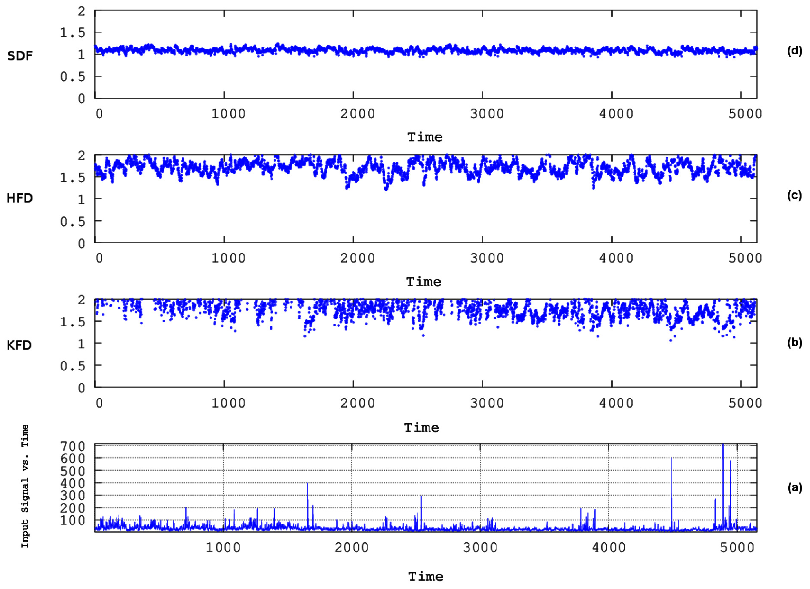
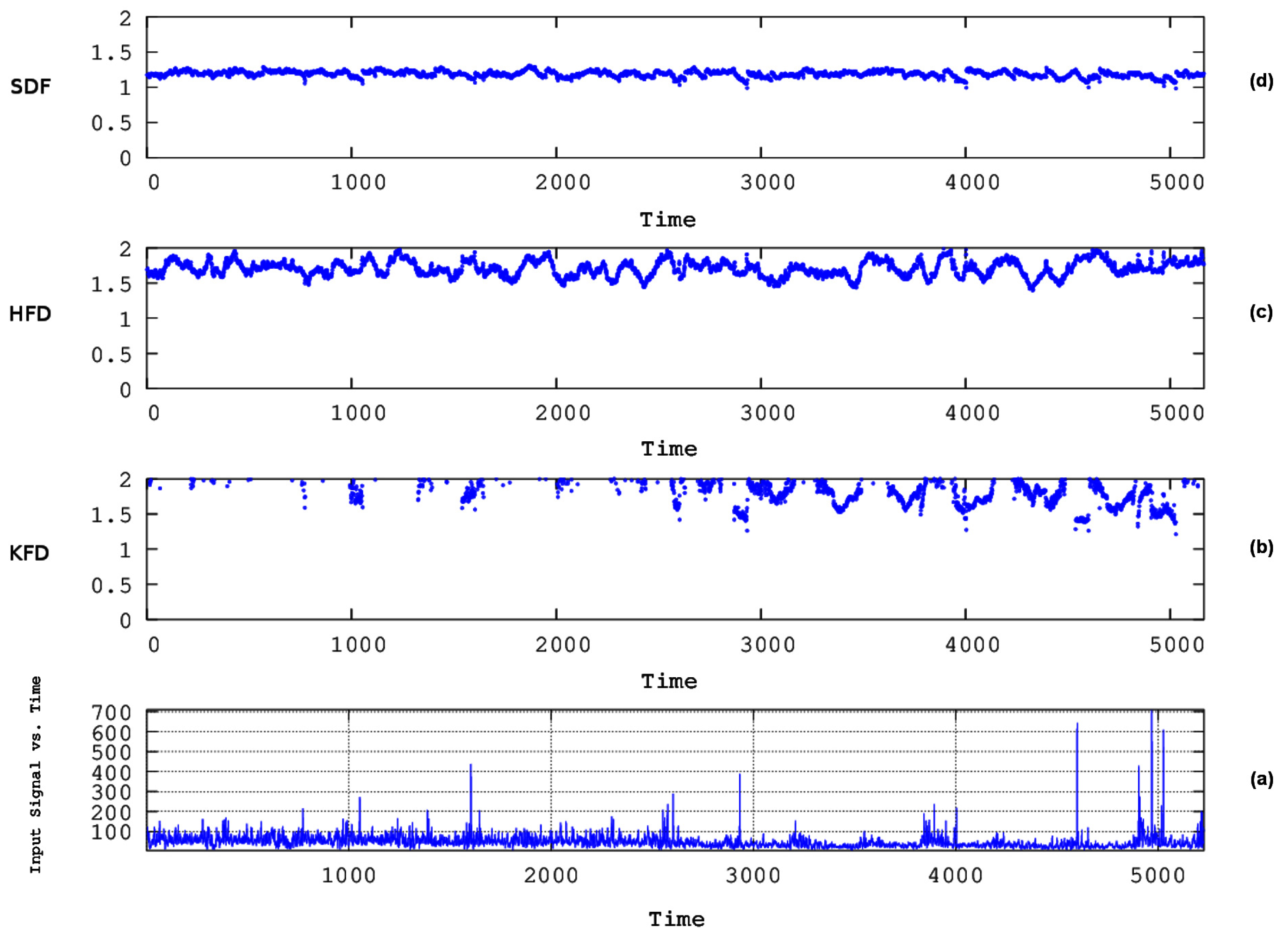
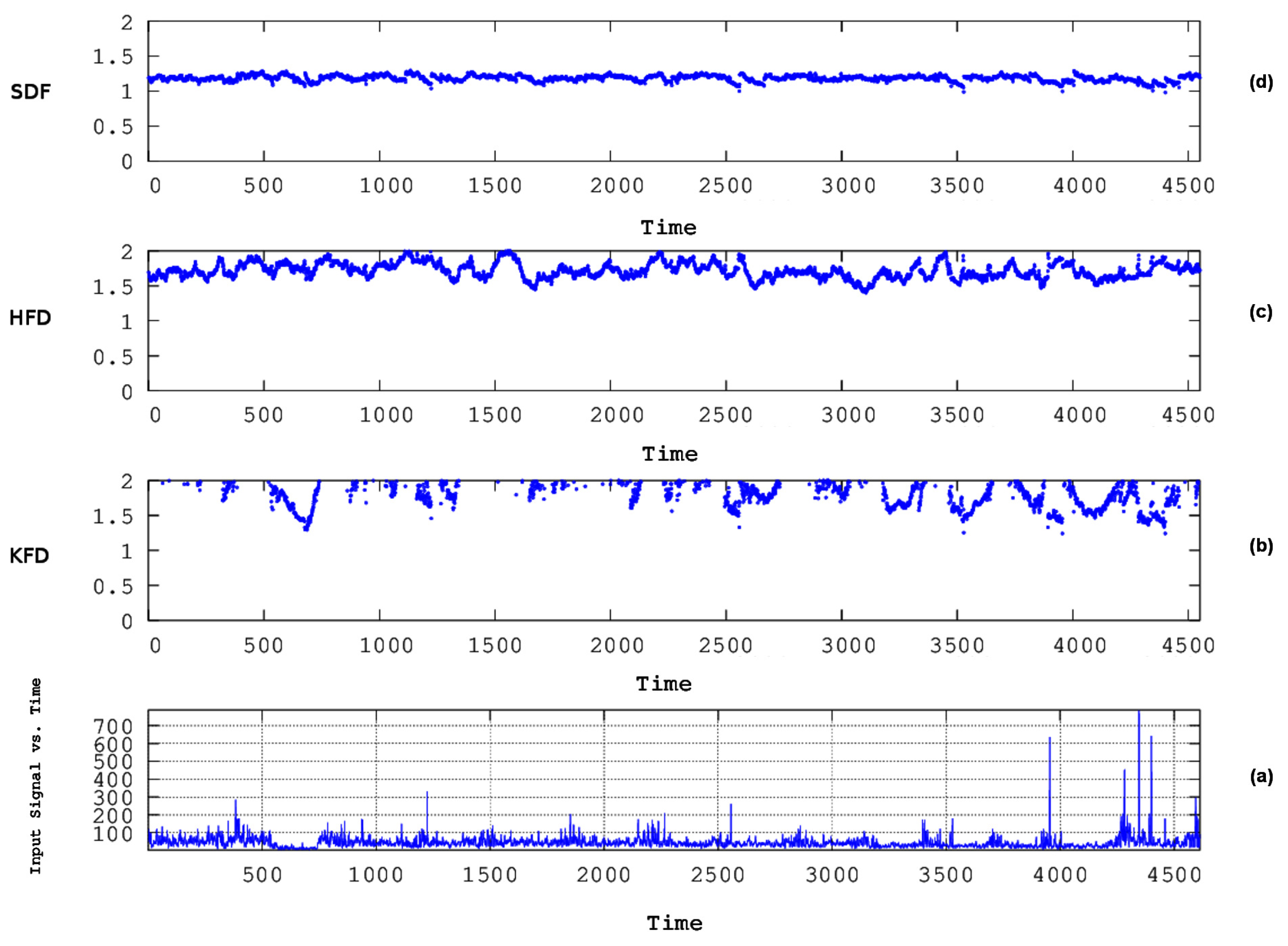
3.3. Fractal-Dimension Analysis

3.3.1. Katz’s Method

Katz’s method is a first approach for the calculation of fractal dimension D. The method [77,78], starts with the transpose array ${[s_1,s_2,\dots ,s_N]}^{⊺}$ of a time series, $s_i$, $i=1,2,\dots ,N$, where $s_i=(t_i,y_i)$ and $y_i$ are the recorded values at sampled time instances $t_i$.

Two sequential time-series points $s_i$ and $s_{i+1}$, represent value pairs ($t_i,y_i$) and ($t_{i+1},y_{i+1}$) with Euclidean distance given by:

$$dist(s_i,s_{i+1})=\sqrt{\left(t_i^2-t_{i+1}^2\right)+\left(y_i^2-y_{i+1}^2\right)}$$

(1)

The total length of the curve of the distances of Equation (1) is:

$$L=\sum _{i=1}^{i=N}dist(s_i,s_{i+1})$$

(2)

Under the assumption that the above curve does not cross itself, its planar extend, d, is given by:

$$d=max(dist(s_i,s_{i+1})),i=2,3,\dots ,N$$

(3)

Katz’s fractal dimension, D, is calculated by Equations (2) and (3) by

$$D=\frac{log(n)}{log(n)+log(D/L)}$$

(4)

where $n=L/\overline{\mathrm{a}}$ and $\overline{\mathrm{a}}$ is the average distance of the points.

3.3.2. Higuchi’s Method

Higuchi’s method is a second approach for the calculation of the fractal dimension D of a time series. As reported in References [79,80] Higuchi ’s fractal dimension D can be calculated for a finite time series recorded at regular intervals $i=1,2\dots N$.

$$y(1),y(2),y(3),\dots ,y(N)$$

(5)

From Series (5) [79,80,81], a new sequence, $y_m^k$, is constructed as follows:

$$y_m^k:y(m),y(m+k),y(m+2k),\dots ,y(m+\left[\frac{N-m}{k}\right]k)$$

(6)

Higuchi [81], defines the length of the curve associated to each time series, $X_m^k$, as follows:

$$L_m(k)=\frac{1}{k}\left(\sum _{i=1}^{\left[\frac{N-m}{k}\right]}y(m+ik)-y(m+(i-1)k)\right)\left(\frac{N-1}{\left[\frac{N-m}{k}\right]k}\right)$$

(7)

where m and k are integers with $m=1,2\dots ,k$ that determine the time lag between samples, the symbol $\left[\dots \right]$ represents the bigger integer part of a value (Gauss notation), and the term

$$\frac{N-1}{\left[\frac{N-m}{k}\right]k}$$

(8)

is a normalisation factor. If a curve is a fractal with fractal dimension D, then the average value $〈L\left(k\right)〉$ of the lengths of Equation (7), is a power law, namely:

$$〈L\left(k\right)〉\propto k^{-D}$$

(9)

Hence, if $〈L\left(k\right)〉$ is plotted versus k, $k=1,2,\dots ,k_{max}$, on a log-log graph, Higuchi’s fractal dimension D can be calculated as a slope of the plot’s linear regression. The interval time is taken as $k=1,‥,k_{max}$ for $k_{max}\le 4$ (e.g., $k=1,2,3,4$, for $k_{max}=4$) and as $k=\left[2^{(j-1)/4}\right]$, $j=11,12,13\dots ,$ for $k>4$ (hence, $k_{max}>4$) and $\left[\dots \right]$ is the Gauss notation [78].

3.3.3. Sevcik Method

Sevcik [82] showed that fractal dimension D can be approximated for the sampled time series of dimension N. According to the Sevcik method, D is estimated from the Hausdorff dimension $D_h$ of a curve as [78]:

$${\displaystyle D_h=\underset{ϵ\to 0}{lim}\left[-\frac{log\left(N\right(ϵ\left)\right)}{log\left(ϵ\right)}\right]}$$

(10)

where $N\left(ϵ\right)$ is the number of segments of length 2$ϵ$ that make up the curve. For a curve of length L, $N\left(ϵ\right)=L/2ϵ$ [78]; hence, $D_h$ becomes:

$${\displaystyle D_h=\underset{ϵ\to 0}{lim}\left[-\frac{log\left(L\right)-log\left(2ϵ\right)}{log\left(ϵ\right)}\right]}$$

(11)

By mapping N points of curve L into a unit square of $N\times N$ cells of a normalised metric space, via double linear transformation, Equation (11) becomes [78,82]:

$${\displaystyle D_h=\underset{N\to \infty }{lim}\left[1+\frac{log\left(L\right)-log\left(2ϵ\right)}{log\left(2\right(N-1\left)\right)}\right]}$$

(12)

The Sevcik fractal dimension is estimated by Equation (12), and the estimation is improved as $N\to \infty$.

3.3.4. Computational Methodology of Fractal Dimension

To calculate fractal dimensions via the methods of Higuchi, Katz, and Sevcik, the following steps were followed:

• The signal was divided into windows of 64 samples (approximately two months’ duration).
• In each segment, the fractal dimension was calculated as follows:
  • Katz’s method: As D from Equation (4) for $n=64$ and $\overline{\mathrm{a}}$ = 1 sample per day, namely, the distance between the points of the series that feed parameter L.
  • Higuchi’s method: As slope D of the best-fit line of the log-log plot of Equation (9), namely, $log(〈L\left(k\right)〉)$ versus $log\left(k\right)$, for $kmax=4$.
  • Sevcik ’s method: As $D=D_h$ from Equation (12) for N = 64, namely, equal to the length of the series in each window.
• The window slid one sample, and Steps (i–ii) were repeated until the end of the signal.

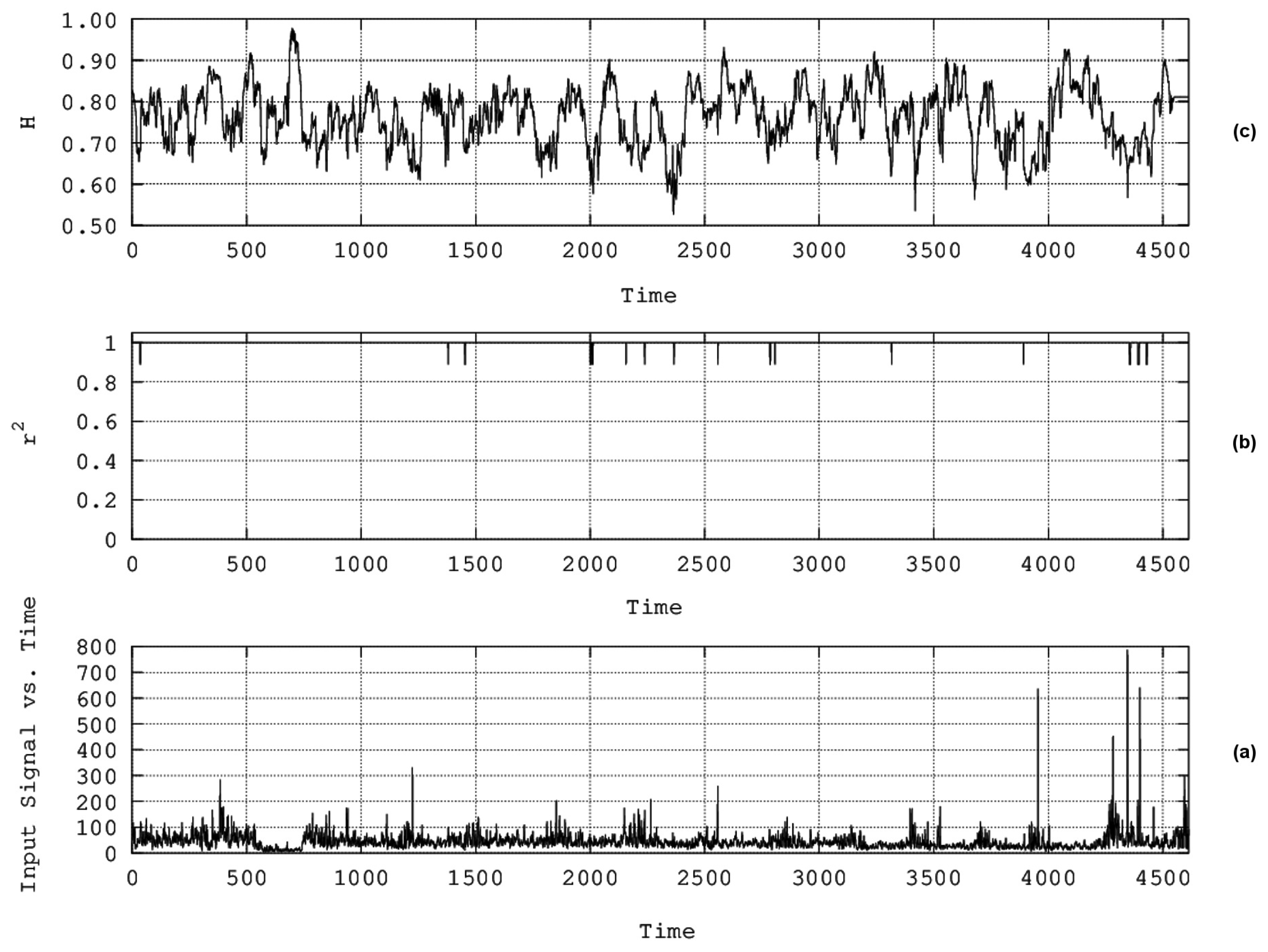
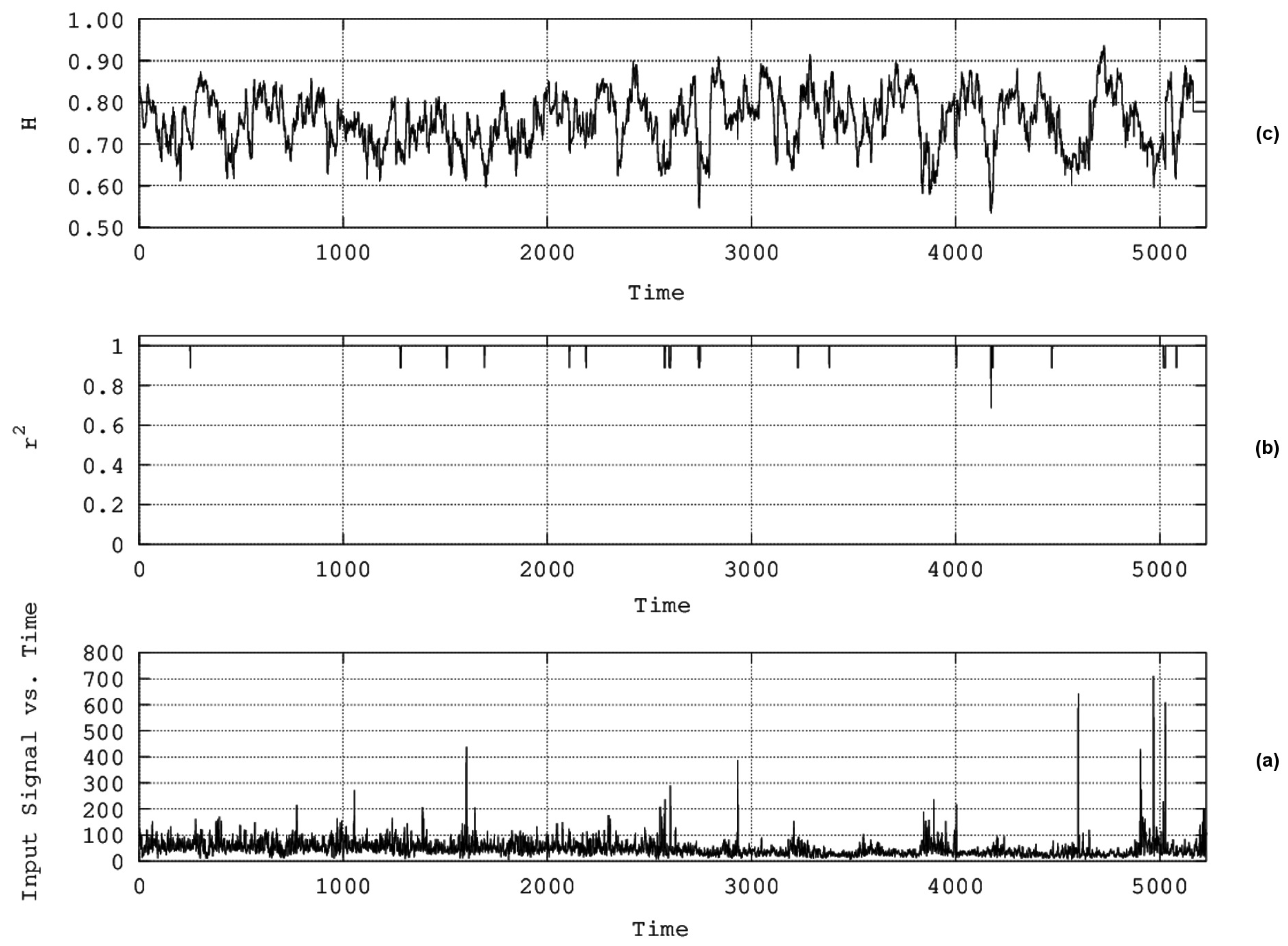
3.4. Rescaled-Range Analysis

R/S analysis was conceptualised by Hurst [62,63], and is a method that can reveal patterns that may be reproduced in the future [41,45,46,47,62,63,64]. The method is based on the transformation of a natural time series, $X\left(N\right)=x\left(1\right),x\left(2\right),\dots ,x\left(N\right)$, to a new time series $y(n,N)$, in a time interval n, where $n=1,2,\dots ,N$ according to Equation (13):

$$y(n,N)=\sum _{i=1}^n(x\left(i\right)-{\langle x\rangle }_N)$$

(13)

In Equation (13), ${\langle x\rangle }_N=\frac{1}{N}{\sum }_{n=1}^{N}x(n)$, is the average value calculated over a time interval N. Variable $y(n,N)$ is known as the accumulated departure of the natural time series.

The R/S (rescaled) range is then calculated from Equation (14) [41,45,46,47,62,63,64]

$$R/S=\frac{R\left(n\right)}{S\left(n\right)}$$

(14)

where $R\left(n\right)$ is the range of $y(n,N)$, namely, the difference between its minimum and maximum values

$$R\left(n\right)=\underset{1⩽n⩽N}{\mathit{max}}y(n,N)-\underset{1⩽n⩽N}{\mathit{min}}y(n,N)$$

(15)

and $S\left(n\right)$ is the standard deviation calculated as:

$$S\left(n\right)=\sqrt{\frac{1}{N}\sum _{n=1}^N{(x\left(n\right)-{\langle x\rangle }_N)}^2}$$

(16)

If there are patterns of long memory hidden in time-series $X\left(N\right)$, $R/S$ exhibits a power-law association with bin size n according to Equation (17):

$$\frac{R\left(n\right)}{S\left(n\right)}=C·n^H$$

(17)

In Equation (17), H is the Hurst exponent, and C is a constant of proportionality.

The logarithmic transformation of Equation (17) yields a linear relation:

$$log(\frac{R\left(n\right)}{S\left(n\right)})=log\left(C\right)+H·log\left(n\right)$$

(18)

The Hurst exponent is estimated by Equation (18) as the slope of the best line fit.

Computational Methodology of R/S Analysis

$R/S$ analysis was utilised according to the following steps:

• The signal was divided in windows of 64 samples (approximately two months’ duration).
• In each segment, the least-square fit was applied to the $\log \left(\frac{R\left(n\right)}{S\left(n\right)}\right)-\log \left(n\right)$ linear representation of Equation (6). Successful representations were considered those exhibiting squares of Spearman’s correlation coefficient above 0.95.
• The window slid one sample, and steps (i–ii) were repeated until the end of the signal.

From the above, the time evolution of the Hurst exponent was derived for every signal under investigation.

4. Results and Discussion

The results from the fractal-analysis methods are presented in Figure 2, Figure 3 and Figure 4. The results from R/S analysis are given in Figure 5, Figure 6 and Figure 7. The reader may recall that the PM₁₀ time series (subfigures (a) of Figure 2, Figure 3, Figure 4, Figure 5, Figure 6 and Figure 7), are lengthy since they refer to all years between 2001 and 2016. Interestingly, during certain periods, relatively high PM₁₀ concentrations were visually observed for all three monitoring stations. Such example areas are around samples 4500 and 5000 in the AGP series, 4500 and 5000 in the LYK series, and 4000 and 4250 in the MAR time series. In spite of the fact that the above sample values are different, the corresponding dates are similar, as computed from the date-sample data of all these series. The above temporal alignment may partially be attributed to the vicinity of the AGP, LYK, and MAR stations. Although the visual observation of data variations may reveal some patterns, it cannot be compared with the outcomes of cutting-edge methods such as neural networks [5,6,7,8,9,10,11,12,13,14,15,16,83] wavelets [4,17,18], and high-level statistics [20,24,28,37]; most importantly, fractal and long-memory methods are more powerful in signal exploration. The latter methods, as already emphasised, are advantageous because they can outline trends that are hidden in the time series. The following issues are significant and should be emphasised. The completeness of the PM₁₀ time series of Figure 2, Figure 3, Figure 4, Figure 5, Figure 6 and Figure 7 are different; 88.2% for the Agia Paraskevi station, 89.5% for the Lykovrissi station, and 78.9% for the Maroussi station. This can be observed from the temporal differentiation of the three time series. The missing values of the time series impose bias to the analysis (e.g., References [52,84] and the related discussion and references), and, for this reason, the above investigators filled the missing data via cubic splines. However, this approach may alter the raw time series and, therefore, if followed, it could bias, or even suppress, any existing fractal and long-memory patterns in the time series. To avoid this type of bias, the PM₁₀ time series (subfigures (a) of Figure 2, Figure 3, Figure 4, Figure 5, Figure 6 and Figure 7) were treated jointly, namely, the missing PM₁₀ values were ignored. This treatment avoids the bias of unavailable data in fractal and long-memory analysis, and is significant according to the following logic: If an N=64-sample window contains missing time-series values, values prior to the missing ones that fill part of the window up to a sample number, n, $n\le$64, are mixed with $N-n$ values recorded after the missing values. In the aspect that n values constitute the present of the time series, whereas $N-n$ values constitute its future, the present is mixed with the future. Considering that sliding one sample forward is finally performed, the past of the series is rematched with its present, which is mixed and also matched with its future. If the time series have hidden fractal and long-memory patterns in critical states, their present is defined not only by their long-term history, but also, most importantly, by their long-lasting future [40,41,42,43,44,45,46,47,61,64,70,71,72,74,85,86]. Under a different aspect, the system is in a non-Markovian state (see above publications and references therein), where its past, present, and future are inevitably linked by interchanged SOC states leading to critical end-points. In view of the above, the joint treatment of missing values is advantageous concerning the delineation of potentially existing fractal and long-memory patterns, since it combines the past, present, and future of the time series in each sliding window. Hereafter, missing values are treated as mentioned above.

The fractal dimensions of Figure 2, Figure 3 and Figure 4 vary. Discrepancies were observed between the D values calculated from the three fractal-dimension algorithms. These discrepancies could be attributed to the different methodology in D calculation between the Katz, Higuchi, and Sevcik methods. Fractal dimensions calculated from the Sevcik method are significantly lower than those of the other two methods. This can be explained by the fact that $N=64$, which is far from the limit of ∞ that the Sevcik method necessitates. The reader should also note that, regarding Katz’s method, only acceptable D values are presented in the (b) subfigures of Figure 2, Figure 3 and Figure 4, namely, only D values in the range of $0\le D\le 2$ are presented. The Hurst exponents of Figure 5, Figure 6 and Figure 7 calculated with R/S analysis, showed temporal variations as well. The D values of Figure 2, Figure 3 and Figure 4 could be compared to the corresponding Hurst exponents of Figure 5, Figure 6 and Figure 7, by utilising the transformation $H=2-D$ [43,45,46,86]. As discussed extensively in Reference [45] and the above publications, the in situ relationship of H and D is linear, but a different relation might be valid. This view seems to be confirmed by the results of Figure 2, Figure 3, Figure 4, Figure 5, Figure 6 and Figure 7, and could be another reason for the addressed discrepancies; however, the latter is outside the scope of this paper.

What is most important from the results of Figure 2, Figure 3, Figure 4, Figure 5, Figure 6 and Figure 7 is that the time variations of D and H are completely different from concurrent time-series variations. This is observed in Figure 2, Figure 3, Figure 4, Figure 5, Figure 6 and Figure 7. This is a significant finding that has been acknowledged by numerous investigators [40,41,42,43,44,45,46,47,61,64,70,71,72,74,85,86,87,88,89,90]. As extensively discussed in the above publications, the employed methods reveal hidden patterns in the time series, and for this reason their time evolution is different from that of the time series. Several windows are spotted with significantly low fractal dimensions and significantly high Hurst exponents. These windows may have been, most probably, linked to PM₁₀ time epochs of critical fractal and long-memory behaviour. Such critical time epochs for the PM₁₀ time series could be the following: (a) continuously changing, power-law fractal, long-memory, or SOC state interactions of the PM₁₀ air-pollution system with various sources of pollutants from industries, vehicles, and energy -generating power stations, combined with complicated physical and chemical processes [24,52]; (b) different small- and large-scale fluctuations of the PM₁₀ time series [52,91,92,93,94], e.g., different types of persistency or antipersistency at the small and large time scales [4]; (c) scalefree fractal PM₁₀ systems with the power-law scaling and long-term memory recognised as a footprint of SOC behaviour [4]; (d) nonlinear low-dimensional chaos dynamics governing the PM₁₀ [95]; (e) external forces, such as meteorological processes and photochemical reactions, which amplify or reduce the contribution of linear and nonlinear mechanisms of ambient pollutant interaction, which further complicate the temporal structure of the dynamics of ambient pollutant concentrations and lead to complex behaviour of air-pollution systems [96]. According to the above argumentation, since the PM₁₀ systems of Figure 2, Figure 3, Figure 4, Figure 5, Figure 6 and Figure 7 had passed from some or numerous critical fractal and long-memory epochs as the ones described above, the most beneficial method to treat the missing values would be the one adopted in this paper, namely, the one that combines the past with the present and the future. These epochs are also linked to SOC states of the PM₁₀ generating system.

The following issues are noteworthy: First, all the windows of Figure 2, Figure 3, Figure 4, Figure 5, Figure 6 and Figure 7 are of 64-sample length, which is the power of two nearest to two months’ length. This is a fair compromise between sufficiently large windows, but not excessively long to include great seasonal changes of atmospheric conditions [97,98,99,100,101]. As found in previous publications [61,64], window lengths above 32 are successful in calculating the Hurst exponents [64] of DFA exponents of electric signals produced by irradiated Quantum Dots [61]. Especially in the latter publication, long-memory analysis was checked versus trivial methodology [91,92,93,94]. Utilisation of very long windows, e.g., above 1024 samples per window, was avoided due to intense seasonal variations’ nonpractical results regarding the time evolution of the hidden trends.

Greatest emphasis, however, should be placed on the following issues. As expressed in recent publications (References [43,44,45] and references therein), in complement to the claims of other publications (e.g., References [38,39,102,103,104] and references therein), it is most significant when analysing the long memory and fractality of a system, not just to identify under- or overthreshold segments, but preferably, to locate under- or overthreshold areas that are commonly found through different chaos-analysis and long-memory methods. In this sense, in order to evaluate the segments of fractal and long-memory behaviour of Figure 2, Figure 3, Figure 4, Figure 5, Figure 6 and Figure 7, it is crucial to set the threshold values for both the fractal dimensions and the Hurst exponents. To achieve this, the output data of the fractal analysis were computationally searched according to user-defined thresholds for common areas of underthreshold values for the fractal dimensions, and overthreshold values for the Hurst exponents from R/S analysis. At first, the threshold for the Hurst exponents derived from R/S analysis was set equal to 0.8 under the constraints that the accepted exponents were above this threshold and simultaneously exhibiting square of Spearman’s correlation coefficient $r^2\ge 0.95$. The threshold for the fractal dimensions calculated from the Sevcik method was set equal to 1.2, since this value corresponds to H = 0.8 from the aforementioned relation $H=2-D$. On the other hand, the outcomes of Katz’s and Higuchi’s methods showed the discrepancies discussed above, in comparison to the dimensions of the Sevcik method. For this reason, the thresholds of the fractal dimensions from Katz’s and Higuchi’s methods were enlarged so as to correspond to Hurst exponents below 0.8, since no fractal dimension was below 1.2 from calculations according to Katz’s and Higuchi’s algorithms. Accounting for this, the fractal-dimension thresholds of Katz’s and Higuchi’s algorithms were taken equal to 1.5, a value significantly lower than the majority of the calculated D values. In order to locate the dates of the common overthreshold areas for H values from the R/S analysis, and the underthreshold values for the D values, proper computational calculations were iterated in the date vectors of the analysed segments under the constraint that the dates of the first sample of each window were arbitrarily attributed to the whole window. This was considered as an acceptable compromise since each window is moved one sample forward and, hence, all dates but the last are covered by analysis windows. The computational iterations to locate common dates with all techniques were repeated for all possible combinations of stations, and were also repeated for all possible combinations of two or more techniques for all stations. The reader should note that this holistic approach to locate common areas in the outputs of different chaos and log-memory analysis techniques that were employed in this paper is not trivial and, when found, the scientific evidence is more in-depth and should be emphasised.

Figure 8 and Figure 9 present the meta-analysis of the chaos and long-memory techniques in accordance to the arguments expressed above. Both Figures show the concurrent meta-analysis results for the data of all three investigated stations. Figure 8 includes all methods of Section 3, while Figure 9 shows all techniques except Katz’s algorithm. As can be observed from Figure 8, there are no common areas simultaneously identified by the three stations when the result data are further processed for coincidences by all techniques of Section 3. This observation can mainly be attributed to the discrepancies in the chaos-analysis results by the three fractal dimension algorithms. Despite this, it is evident from Figure 8 that the results coincide for the data of two stations. Twelve dates were identified from combination analysis of the results of the Agia Paraskevi and Lykovrissi stations, and 36 for the the combination of data from the Agia Paraskevi and Maroussi stations. Lykovrissi results versus Maroussi results did not show common areas. On the other hand, results were significantly enhanced when the outputs from Katz’s algorithm were not included in the meta-analysis. As can be observed from Figure 9, 16 common areas are common for the data from all stations. The actual dates of Figure 9 are presented in

Table 1. Coincidence dates of common segments of Figure 9.

Dates
2007-7-28	2010-6-7	2010-6-9	2010-6-10
2010-6-11	2010-6-13	2010-6-16	2010-6-28
2013-8-18	2013-8-31	2013-9-1	2013-9-2
2013-9-3	2013-9-4	2013-9-8	2013-9-9

, as this is considered the most significant output. The combinations of fractal methods only, as well as of two fractal methods and R/S analysis, did not present more than two coincident dates. These findings are due to the fact that Katz’s algorithm produces fewer D values in the range of $0\le D\le 2$, a fact that might be the source of the observed deviations. On the other hand, despite that Sevcik’s N is far from ∞, the results of Sevcik’s method are closer to the results of R/S analysis, because the $H=2-D$ relation seems to be functional for the combination of only these techniques. However, as expressed in the discussion above, the scientific validity of the outcomes of the fractal and long-memory analysis techniques are more in-depth in the identified common areas by the combination of several methods. In this sense, the results of Figure 8 and Figure 9 and Table 1, are, to the view of the authors, the most significant. As also expressed in the discussion, other investigators published the view of signifying results from only one method. In this view, it is interesting to note that, with the utilised threshold criteria, R/S analysis showed 1902 long-memory segments for the Agia Paraskevi station, 1425 for the Lykovrissi station, and 1559 for the Maroussi station. As also expressed in recent publications (References [43,44,45] and references therein), identification on many H-over-threshold segments is trivial for R/S analysis. Regarding the fractal-dimension analysis, e.g., from the data of the Lykovrissi station, 411 fractal segments were recognised by Katz’s method, 889 by Higuchi’s method, and 2881 by Sevcik’s method. An analogous number of segments were identified by the data from the other two stations as well. This latter finding reinforces the aspect expressed in this paper and followed in the postanalysis of the results of the fractal and long-memory methods; every technique showed several areas of fractal and long-memory behaviour. The evidence is stronger only for those of Figure 8 and Figure 9 and Table 1. The expressed aspects, the employed methodology, together with the presented results and discussion, indicate that the combination of several methods is a very promising tool for analysing PM air-pollution data.

5. Conclusions

The following summarises the most significant results:

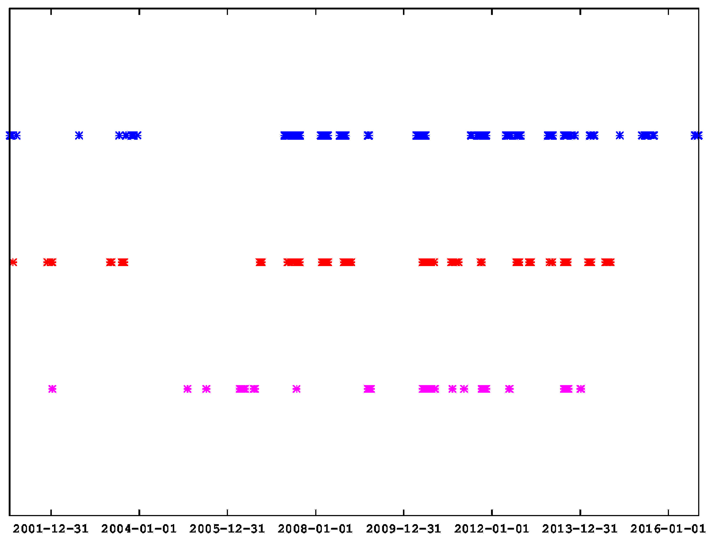
• The algorithms of Katz, Higuchi, and Sevcik were employed together with R/S analysis via sliding windows of two months’ duration to investigate the existence of chaos and long memory in three 16-year-long PM₁₀ concentration time series recorded in Athens, Greece.
• Several segments were found with dynamical complex fractal behaviour and long memory. Via specific thresholds, computational calculations were performed on all possible combinations of two or more techniques for the data of all stations under study. The best combination of methods for the data of all stations was the one not including Katz’s algorithm in the meta-analysis.
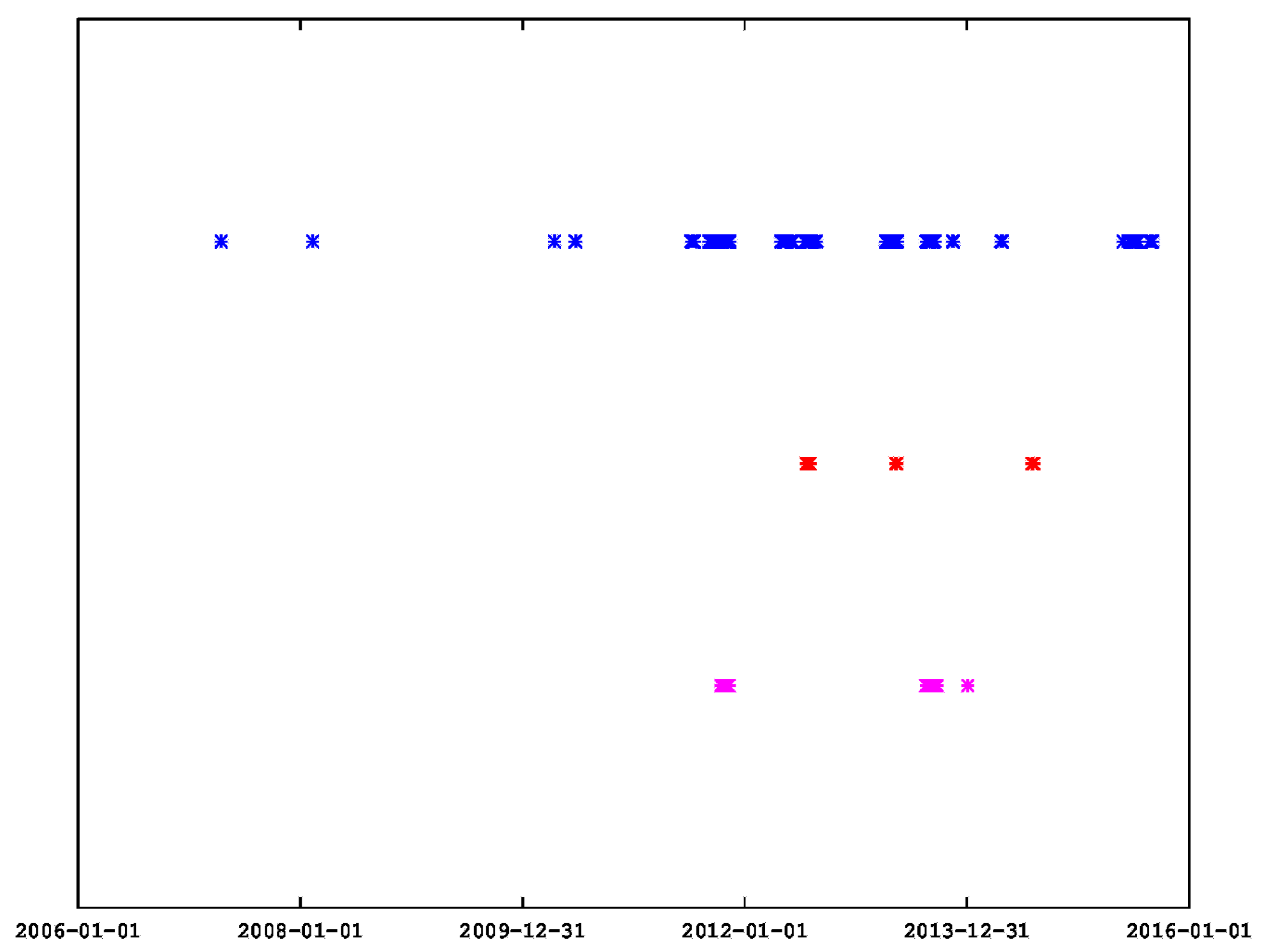
• Twelve dates of coincidence were identified from this combination of techniques.

References

1. Chan, C.K.; Yao, X. Air pollution in mega cities in China. Atmos. Environ. 2008, 42, 1–42. [Google Scholar]
2. Fang, M.; Chan, C.K.; Yao, X.H. Managing air quality in a rapidly developing nation: China. Atmos. Environ. 2009, 43, 79–86. [Google Scholar]
3. Liu, N.; Yu, Y.; He, J.; Zhao, S. Integrated modeling of urban-scale pollutant transport: Application in a semi-arid urban valley, Northwestern China. Atmos. Pollut. Res. 2013, 4, 306–314. [Google Scholar]
4. Liu, Z.; Wang, L.; Zhu, H. A time-scaling property of air pollution indices: A case study of Shanghai. China Atmos. Pollut. Res. 2015, 6, 886–892. [Google Scholar]
5. Ibarra-Berastegi, G.; Elias, A.; Barona, A.; Saenz, J.; Ezcurra, A.; de Argandona, J.D. From diagnosis to prognosis for forecasting air pollution using neural networks: Air pollution monitoring in Bilbao. Environ. Model. Softw. 2008, 23, 622–637. [Google Scholar]
6. Kourentzes, N.; Barrow, D.K.; Crone, S.F. Neural network ensemble operators for time series forecasting. Expert Syst. Appl. 2014, 41, 4235–4244. [Google Scholar]
7. Pérez, P.; Trier, A.; Reyes, J. Prediction of PM2.5 concentrations several hours in advance using neural networks in Santiago, Chile. Atmos. Environ. 2000, 34, 1189–1196. [Google Scholar]
8. Hooyberghs, J.; Mensink, C.; Dumont, G.; Fierens, F.; Brasseur, O. A neural network forecast for daily average PM10 concentrations in Belgium. Atmos. Environ. 2005, 39, 3279–3289. [Google Scholar]
9. Grivas, G.; Chaloulakou, A. Artificial neural network models for prediction of PM10 hourly concentrations in the Greater Area of Athens, Greece. Atmos. Environ. 2006, 40, 1216–1229. [Google Scholar]
10. Barai, S.V.; Dikshit, A.K.; Sharma, S. Neural Network Models for Air Quality Prediction: A Comparative Study. In Soft Computing in Industrial Applications; Saad, A., Dahal, K., Sarfraz, M., Roy, R., Eds.; Springer: Berlin/Heidelberg, Germany, 2007; Volume 39. [Google Scholar]
11. Díaz-Robles, L.A.; Ortega, J.C.; Fu, J.S.; Reed, G.D.; Chow, J.C.; Watson, J.G.; Moncada-Herrera, J. A hybrid ARIMA and artificial neural networks model to forecast particulate matter in urban areas: The case of Temuco, Chile. Atmos. Environ. 2008, 42, 8331–8340. [Google Scholar]
12. Antanasijević, D.Z.; Pocajt, V.V.; Povrenović, D.S.; Ristić, M.D.; Perić-Grujić, A.A. PM10 emission forecasting using artificial neural networks and genetic algorithm input variable optimization. Sci. Total. Environ. 2013, 443, 511–519. [Google Scholar] [PubMed]
13. Moustris, K.P.; Ziomas, I.C.; Paliatsos, A.G. 3-Day-Ahead Forecasting of Regional Pollution Index for the pollutants NO2, CO, SO2 and O3 using Artificial Neural Networks in Athens, Greece. Water Air Soil. Pollut. 2010, 224, 29–43. [Google Scholar]
14. Moustris, K.P.; Nastos, P.T.; Larisssi, I.K.; Paliatsos, A.G. Application of Multiple Linear Regression Models and Artificial Neural Networks on the surface ozone forecast in the greater Athens area, Greece. Adv. Meteorol. 2012, 2012, 1–8. [Google Scholar]
15. Moustris, K.P.; Larisssi, I.K.; Nastos, P.T.; Koukouletsos, K.V.; Paliatsos, A.G. Development and Application of Artificial Neural Network Modeling in Forecasting PM10 Levels in a Mediterranean City. Water Air Soil Pollut. 2013, 224. [Google Scholar]
16. Moustris, K.P.; Proias, G.T.; Larisssi, I.K.; Nastos, P.T.; Koukouletsos, K.V.; Paliatsos, A.G. Air quality prognosis using artificial neural networks modeling in the urban environment of Volos, Central Greece. Fres. Environ. Bull. 2014, 13, 2967–2975. [Google Scholar]
17. Hong, L. Decomposition and forecast for financial time series with high-frequency based on empirical mode decomposition. Energy Procedia 2011, 5, 1333–1340. [Google Scholar]
18. Maheswaran, R.; Khosa, R. Wavelet Volterra Coupled Models for forecasting of nonlinear and non–stationary time series. Neurocomputing 2015, 149, 1074–1084. [Google Scholar]
19. Sefidmazgi, G.; Sayemuzzaman, M.; Homaifar, M.; Jha, M.K.; Liess, S. Trend analysis using non-stationary time series clustering based on the finite element method. Nonlinear Process. Geophys. 2014, 21, 605–615. [Google Scholar]
20. Lorentzen, T. Statistical analysis of temperature data sampled at Station-M in the Norwegian Sea. J. Mar. Syst. 2014, 130, 31–45. [Google Scholar]
21. Samet, H.; Marzbani, F. Quantizing the deterministic nonlinearity in wind speed time series. Renew. Sustain. Energy Rev. 2014, 39, 1143–1154. [Google Scholar]
22. Chelani, A.B. Persistence analysis of extreme CO, NO2 and O3 concentrations in ambient air of Delhi. Atmos. Res. 2012, 108, 128–134. [Google Scholar]
23. Gan, M.; Cheng, Y.; Liu, K.; Zhang, G.L. Seasonal and trend time series forecasting based on a quasi-linear autoregressive model. Appl. Soft Comput. 2014, 24, 13–18. [Google Scholar]
24. Shi, K.; Liu, C.Q.; Ai, N.S.; Zhang, X.H. Using three methods to investigate time-scaling properties in air pollution indexes time series. Nonlinear Anal. Real World Appl. 2008, 9, 693–707. [Google Scholar]
25. Lee, C.K.; Ho, D.S.; Yu, C.C.; Wang, C.C.; Hsiao, H.T. Simple multifractal cascade model for the air pollutant concentration time series. Environmetrics 2003, 14, 255–269. [Google Scholar]
26. Lau, J.C.; Hung, W.T.; Yuen, D.D.; Cheung, C.S. Long-memory characteristics of urban roadside air quality. Transp. Res. D 2009, 14, 353–359. [Google Scholar]
27. Perez, I.A.; Sanchez, M.L.; Garcia, M.A.; Paredes, V. Persistence analysis of CO2 concentrations recorded at a rural site in the upper Spanish plateau. Atmos. Res. 2011, 100, 45–50. [Google Scholar]
28. Scott, L.S.; Varian, H.R. Predicting the present with bayesian structural time series. Int. J. Math. Model. Numer. Optim. 2014, 5, 4–23. [Google Scholar]
29. Shi, K.; Liu, C.Q.; Ai, N.S. Monofractal and multifractal approaches in investigating temporal variation of air pollution indexes. Fractals 2009, 17, 513–521. [Google Scholar]
30. Varotsos, C.; Kirk-Davidoff, D. Long-memory processes in ozone and temperature variations at the region 60 0 S–600 N. Atmos. Chem. Phys. 2006, 6, 4093–4100. [Google Scholar]
31. Varotsos, C.; Ondov, J.; Efstathiou, M. Scaling properties of air pollution in Athens, Greece and Baltimore, Maryland. Atmos. Environ. 2005, 39, 4041–4047. [Google Scholar]
32. Varotsos, C.A.; Ondov, J.M.; Cracknell, A.P.; Efstathiou, M.N.; Assimakopoulos, M.N. Long-range persistence in global aerosol index dynamics. Int. J. Remote Sens. 2006, 27, 3593–3603. [Google Scholar]
33. Yuval; Broday, D.M. Studying the time scale dependence of environmental variables predictability using fractal analysis. Environ. Sci. Technol. 2010, 44, 4629–4634. [Google Scholar] [PubMed]
34. Weng, Y.C.; Chang, N.B.; Lee, T.Y. Nonlinear time series analysis of ground-level ozone dynamics in Southern Taiwan. J. Environ. Manag. 2008, 87, 405–414. [Google Scholar]
35. Windsor, H.L.; Toumi, R. Scaling and persistence of UK pollution. Atmos. Environ. 2001, 35, 4545–4556. [Google Scholar]
36. Zhu, J.; Liu, Z. Long-range persistence of acid deposition. Atmos. Environ. 2003, 37, 613. [Google Scholar]
37. Schlink, U.; Herbarth, O.; Richter, M.; Dorling, S.; Nunnari, G.; Cawley, G.; Pelikan, E. Statistical models to assess the health effects and to forecast ground—Level ozone. Environ. Model. Softw. 2006, 21, 547–558. [Google Scholar]
38. Eftaxias, K.; Panin, V.; Deryugin, Y. Evolution-EM signals before earthquakes in terms of mesomechanics and complexity. Phys. Chem. Earth 2007, 29, 445–451. [Google Scholar]
39. Eftaxias, K.; Balasis, G.; Contoyiannis, Y.; Papadimitriou, C.; Kalimeri, M. Unfolding the procedure of characterizing recorded ultra low frequency, kHZ and MHz electromagnetic anomalies prior to the L’Aquila earthquake as pre-seismic one—Part 2. Nat. Hazard Earth Syst. 2010, 10, 275–294. [Google Scholar]
40. Nikolopoulos, D.; Petraki, E.; Marousaki, A.; Potirakis, S.; Koulouras, G.; Nomicos, C.; Panagiotaras, D.; Stonhamb, J.; Louizi, A. Environmental monitoring of radon in soil during a very seismically active period occurred in South West Greece. J. Environ. Monit. 2012, 14, 564–578. [Google Scholar] [PubMed]
41. Nikolopoulos, D.; Cantzos, D.; Petraki, E.; Yannakopoulos, P.H.; Nomicos, C. Traces of long-memory in pre-seismic MHz electromagnetic time series-Part1: Investigation through the R/S analysis and time-evolving spectral fractals. J. Earth Sci. Clim. Chang. 2016, 7, 359. [Google Scholar]
42. Nikolopoulos, D.; Petraki, E.; Cantzos, D.; Yannakopoulos, P.H.; Panagiotaras, D.; Nomicos, C. Fractal Analysis of Pre-Seismic Electromagnetic and Radon Precursors: A Systematic Approach. J. Earth Sci. Clim. Chang. 2016, 7, 1–11. [Google Scholar]
43. Nikolopoulos, D.; Matsoukas, C.; Yannakopoulos, P.H.; Petraki, E.; Cantzos, D.; Nomicos, C. Long-Memory and Fractal Trends in Variations of Environmental Radon in Soil: Results from Measurements in Lesvos Island in Greece. J. Earth Sci. Clim. Chang. 2018, 9, 1–11. [Google Scholar]
44. Nikolopoulos, D.; Yannakopoulos, P.H.; Petraki, E.; Cantzos, D.; Nomicos, C. Long-Memory and Fractal Traces in kHz-MHz Electromagnetic Time Series Prior to the ML = 6.1, 12/6/2007 Lesvos, Greece Earthquake: Investigation through DFA and Time-Evolving Spectral Fractals. J. Earth Sci. Clim. Chang. 2018, 9, 1–15. [Google Scholar]
45. Petraki, E. Electromagnetic Radiation and Radon-222 Gas Emissions as Precursors of Seismic Activity. Ph.D. Thesis, Department of Electronic and Computer Engineering, Brunel University, London, UK, 2016. [Google Scholar]
46. Petraki, E.; Nikolopoulos, D.; Fotopoulos, A.; Panagiotaras, D.; Koulouras, G.; Zisos, A.; Nomicos, C.; Louizi, A.; Stonham, J. Self-organised critical features in soil radon and MHz electromagnetic disturbances: Results from environmental monitoring in Greece. Appl. Radiat. Isotop. 2013, 72, 39–53. [Google Scholar]
47. Nikolopoulos, D.; Petraki, E.; Nomicos, C.; Koulouras, G.; Kottou, S.; Yannakopoulos, P.H. Long-Memory Trends in Disturbances of Radon in Soil Prior ML = 5.1 Earthquakes of 17 November 2014 Greece. J. Earth Sci. Clim. Chang. 2015, 6, 1–11. [Google Scholar]
48. Telesca, L.; Lapenna, V.; Vallianatos, F. Monofractal and multifractal approaches in investigating scaling properties in temporal patterns of the 1983–2000 seismicity in the Western Corinth Graben, Greece. Phys. Earth Planet. Int. 2002, 131, 63–79. [Google Scholar]
49. Telesca, L.; Lapenna, V.; Macchiato, M. Mono- and multi-fractal investigation of scaling properties in temporal patterns of seismic sequences. Chaos Solit. Fract. 2004, 19, 1–15. [Google Scholar]
50. Lee, C.K.; Juang, L.C.; Wang, C.C.; Liao, Y.Y.; Yu, C.C.; Liu, Y.C.; Ho, D.S. Scaling characteristics in ozone concentration time series (OCTS). Chemosphere 2006, 62, 934–946. [Google Scholar] [PubMed]
51. Xue, Y.; Pan, W.; Lu, W.z.; He, H.D. Multifractal nature of particulate matters (PMs) in Hong Kong urban air. Sci. Total Environ. 2015, 532, 744–751. [Google Scholar] [PubMed]
52. Dong, Q.; Wang, Y.; Li, P. Multifractal behavior of an air pollutant time series and the relevance to the predictability. Environ. Pollut. 2017, 222, 444–457. [Google Scholar] [PubMed]
53. Vlachogianni, A.; Kassomenos, P. One day ahead prediction of morning max CO concentration in Athens, Greece. In Proceedings of the International Conference on Environmental Management Engineering, Planning and Economics, Skiathos Island, Greece, 2–4 June 2007; pp. 2411–2416. [Google Scholar]
54. Larissi, I.K.; Koukouletsos, K.V.; Moustris, K.P.; Antoniou, A.; Paliatsos, A.G. PM10 concentration levels in the greater Athens area, Greece. Fresen. Environ. Bull. 2010, 19, 226–231. [Google Scholar]
55. Nastos, P.T.; Philandras, C.M.; Paliatsos, A.G. Fourier analysis of the mean monthly NOx concentrations in the Athens basin. Glob. Nest 2002, 4, 145–152. [Google Scholar]
56. Mandelbrot, B.B.; Ness, J.W.V. Fractional Brownian motions, fractional noises and applications. J. Soc. Ind. Appl. Math. 1968, 10, 422–437. [Google Scholar]
57. Morales, I.O.; Landa, O.; Fossion, R.; Frank, A. Scale invariance, self-similarity and critical behaviour in classical and quantum system. J. Phys. Conf. Ser. 2012, 380, 012020. [Google Scholar]
58. Musa, M.; Ibrahim, K. Existence of long memory in ozone time series. Sains Malays. 2012, 41, 1367–1376. [Google Scholar]
59. May, R.M. Simple mathematical models with very complicated dynamics. Nature 1976, 261, 459–467. [Google Scholar] [PubMed]
60. Sugihara, G.; May, R. Nonlinear forecasting as a way of distinguishing chaos from measurement error in time series. Nature 1990, 344, 734–741. [Google Scholar] [PubMed]
61. Nikolopoulos, D.; Valais, I.; Michail, C.; Bakas, A.; Fountzoula, C.; Cantzos, D.; Bhattacharyya, D.; Sianoudis, I.; Fountos, G.; Yannakopoulos, P.H.; et al. Radioluminescence properties of the CdSe/ZnS Quantum Dot nanocrystals with analysis of long-memory trends. Radiat. Meas. 2016, 92, 19–31. [Google Scholar]
62. Hurst, H. Long term storage capacity of reservoirs. Trans. Am. Soc. Civ. Eng. 1951, 116, 770–808. [Google Scholar]
63. Hurst, H.; Black, R.; Simaiki, Y. Long-term Storage: An Experimental Study; Constable: London, UK, 1965. [Google Scholar]
64. Nikolopoulos, D.; Petraki, E.; Vogiannis, E.; Chaldeos, Y.; Giannakopoulos, P.; Kottou, S.; Nomicos, C.; Stonham, J. Traces of self-organisation and long-range memory in variations of environmental radon in soil: Comparative results from monitoring in Lesvos Island and Ileia (Greece). J. Radioanal. Nucl. Chem. 2014, 299, 203–219. [Google Scholar]
65. Lopez, T.; Martınez-Gonzalez, C.; Manjarrez, J.; Plascencia, N.; Balankin, A. Fractal Analysis of EEG Signals in the Brain of Epileptic Rats, with and without Biocompatible Implanted Neuroreservoirs. AMM 2009, 15, 127–136. [Google Scholar]
66. Kilcik, A.; Anderson, C.; Rozelot, J.; Ye, H.; Sugihara, G.; Ozguc, A. Nonlinear Prediction of Solar Cycle 24. Astrophys. J. 2009, 693, 1173–1177. [Google Scholar]
67. Gilmore, M.; Yu, C.; Rhodes, T.; Peebles, W. Investigation of rescaled range analysis, the Hurst exponent, and long-time correlations in plasma turbulence. Phys. Plasmas 2002, 9, 1312–1317. [Google Scholar]
68. Granero, M.S.; Segovia, J.T.; Perez, J.G. Some comments on Hurst exponent and the long memory processes on capital Markets. Phys. A 2008, 387, 5543–5551. [Google Scholar]
69. Dattatreya, G. Hurst Parameter Estimation from Noisy Observations of Data Traffic Traces. In Proceedings of the 4th WSEAS International Conference on Electronics, Control And Signal Processing, Miami, FL, USA, 17–19 November 2005; pp. 193–198. [Google Scholar]
70. Contoyiannis, Y.F.; Diakonos, F.K.; Kapiris, P.G.; Peratzakis, A.S.; Eftaxias, K.A. Intermittent dynamics of critical pre-seismic electromagnetic fluctuations. Phys. Chem. Earth 2004, 29, 397–408. [Google Scholar]
71. Fujinawa, Y.; Takahashi, K. Electromagnetic radiations associated with major earthquakes. Phys. Earth Planet. Int. 1998, 105, 249–259. [Google Scholar]
72. Hayakawa, M.; Ida, Y.; Gotoh, K. Multifractal analysis for the ULF geomagnetic data during the Guam earthquake. Electromagnetic Compatibility and Electromagnetic Ecology. In Proceedings of the IEEE 6th International Symposium on Electromagnetic Compatibility and Electromagnetic Ecology, Saint Petersburg, Russia, 21–24 June 2005; pp. 239–243. [Google Scholar]
73. Hayakawa, M. VLF/LF radio sounding of ionospheric perturbations associated with earthquakes. Sensors 2007, 7, 1141–1158. [Google Scholar]
74. Kalimeri, M.; Papadimitriou, C.; Balasis, G.; Eftaxias, K. Dynamical complexity detection in pre-seismic emissions using non-additive Tsallis entropy. Phys. A 2008, 387, 1161–1172. [Google Scholar]
75. Li, X.; Polygiannakis, J.; Kapiris, P.; Peratzakis, A.; Eftaxias, K.; Yao, X. Fractal spectral analysis of pre-epileptic seizures in terms of criticality. J. Neural Eng. 2005, 2, 11–16. [Google Scholar] [PubMed]
76. Rehman, S.; Siddiqi, A. Wavelet based Hurst exponent and fractal dimensional analysis of Saudi climatic dynamics. Chaos Solit. Fract. 2009, 39, 1081–1090. [Google Scholar]
77. Katz, M. Fractals and the analysis of waveforms. Comput. Biol. Med. 1988, 18, 145–156. [Google Scholar] [PubMed]
78. Raghavendra, B.; Dutt, D.N. Computing Fractal Dimension of Signals using Multiresolution Box-counting Method. Int. J. Electr. Comput. Energ. Electron. Commun. Eng. 2010, 4, 183–198. [Google Scholar]
79. De la Torre, F.C.; Ramirez-Rojas, A.; Pavia-Miller, C.; Angulo-Brown, F.; Yepez, E.; Peralta, J.A. A comparison between spectral and fractal methods in electrotelluric time series. Revista Mexicana Fisica 1999, 45, 298–302. [Google Scholar]
80. De la Torre, F.C.; Gonzaalez-Trejo, J.; Real-Ramírez, C.; Hoyos-Reyes, L. Fractal dimension algorithms and their application to time series associated with natural phenomena. J. Phys. Conf. Ser. 2013, 475, 1–10. [Google Scholar]
81. Higuchi, T. Approach to an irregular time series on basis of the fractal theory. Phys. D 1988, 31, 277–283. [Google Scholar]
82. Sevcik, C. On fractal dimension of waveforms. Chaos Solit. Fract. 2006, 27, 579–580. [Google Scholar]
83. Benjamin, N.; Sharma, S.; Pendharker, U.; Shrivastava, J.K. Air quality prediction using artificial neural network. Int. J. Chem. Stud. 2014, 2, 7–9. [Google Scholar]
84. Carrizosa, E.; Olivares-Nadal, A.V.; Ramírez-Cobo, P. Time series interpolation via global optimization of moments fitting. Eur. J. Oper. Res. 2013, 230, 97–112. [Google Scholar]
85. Eftaxias, K. Footprints of non-extensive Tsallis statistics, self-affinity and universality in the preparation of the L’Aquila earthquake hidden in a pre-seismic EM emission. Phys. A 2010, 389, 133–140. [Google Scholar]
86. Petraki, E.; Nikolopoulos, D.; Fotopoulos, A.; Panagiotaras, D.; Nomicos, C.; Yannakopoulos, P.; Kottou, S.; Zisos, A.; Louizi, A.; Stonham, J. Long-range memory patterns in variations of environmental radon in soil. Anal. Methods 2013, 5, 4010–4020. [Google Scholar]
87. Varotsos, P.; Sarlis, N.; Skordas, E. Magnetic field variations associated with SES. The instrumentation used for investigating their detectability. Proc. Jpn. Acad. Ser. B 2001, 77, 87–92. [Google Scholar]
88. Varotsos, P.; Sarlis, N.; Skordas, E. Long-range correlations in the electric signals that precede rupture: Further investigations. Phys. Rev. E 2003, 67, 021109. [Google Scholar]
89. Varotsos, P.; Sarlis, N.; Skordas, E. Scale-specific order parameter fluctuations of seismicity in natural time before mainshocks. EPL 2011, 96, 1–6. [Google Scholar]
90. Varotsos, P.; Sarlis, N.; Skordas, E. Identifying the occurrence time of an impending major earthquake: A review. Earthq. Sci. 2017, 30, 209–218. [Google Scholar]
91. Peng, C.; Mietus, J.; Havlin, S.; Stanley, H.; Goldberger, A. Long-range anti-correlations and non-Gaussian behavior of the heartbeat. Phys. Rev. Lett. 1993, 70, 1343–1346. [Google Scholar]
92. Peng, C.; Buldyrev, S.; Simons, M.; Havlin, S.; Stanley, H.; Goldberger, A. On the mosaic organization of DNA sequences. Phys. Rev. E 1994, 49, 1685–1689. [Google Scholar]
93. Peng, C.; Havlin, S.; Stanley, H.; Goldberger, A. Quantification of scaling exponents and crossover phenomena in nonstationary heartbeat time series. Chaos 1995, 5, 82–87. [Google Scholar] [PubMed]
94. Peng, C.; Hausdor, J.; Havlin, S.; Mietus, J.; Stanley, H.; Goldberger, A. Multiple-time scales analysis of physiological time series under neural control. Phys. A 1998, 249, 491–500. [Google Scholar]
95. Khokhlov, V.N.; Glushkov, A.V.; Loboda, N.S.; Bunyakova, Y.Y. Short-range forecast of atmospheric pollutants using non-linear prediction method. Atmos. Environ. 2008, 42, 7284–7292. [Google Scholar]
96. Yu, H.L.; Lin, Y.C.; Sivakumar, B.; Kuo, Y. A study of the temporal dynamics of ambient particulate matter using stochastic and chaotic techniques. Atmos. Environ. 2015, 69, 37–45. [Google Scholar]
97. Furuya, K.; Kudo, Y.; Okinaga, K.; Yamuki, M.; Takahashi, S.; Araki, Y.; Hisamatsu, Y. Seasonal variation and their characterization of suspended particulate matter in the air of subway stations. J. Trace Microprobe Tech. 2001, 19, 469–485. [Google Scholar]
98. Hand, J.L.; Schichtel, B.A.; Pitchford, M.; Malm, W.C.; Frank, N.H. Seasonal composition of remote and urban fine particulate matter in the United States. J. Geophys. Res. 2012, 117, D05209. [Google Scholar]
99. Ho, K.F.; Lee, S.C.; Cao, J.J.; Chow, J.C.; Watson, J.G.; Chan, C.K. Seasonal variations and mass closure analysis of particulate matter in Hong Kong. Sci. Total Environ. 2006, 355, 276–287. [Google Scholar] [PubMed]
100. Koelemeijer, R.B.A.; Homan, C.D.M. Comparison of spatial and temporal variations of aerosol optical thickness and particulate matter over Europe. Atmos. Environ. 2006, 40, 5304–5315. [Google Scholar]
101. Mayzaud, P.; Chanut, J.P.; Ackman, R.G. Seasonal changes of the biochemical composition of marine particulate matter with special reference to fatty acids and sterols. Mar. Ecol. Prog. Ser. 1989, 56, 189–204. [Google Scholar]
102. Eftaxias, K.; Sgrigna, V.; Chelidze, T. Mechanical and electromagnetic phenomena accompanying preseismic deformation: From laboratory to geophysical scale. Tectonophysics 2007, 341, 1–5. [Google Scholar]
103. Eftaxias, K.; Contoyiannis, Y.; Balasis, G.; Karamanos, K.; Kopanas, J.; Antonopoulos, G.; Koulouras, G.; Nomicos, C. Evidence of fractional-Brownian-motion-type asperity model for earthquake generation in candidate pre-seismic electromagnetic emissions. Nat. Hazard Earth Syst. 2008, 8, 657–669. [Google Scholar]
104. Eftaxias, K.; Balasis, G.; Contoyiannis, Y.; Papadimitriou, C.; Kalimeri, M.; Athanasopoulou, L.; Nikolopoulos, S.; Kopanas, J.; Antonopoulos, G.; Nomicos, C. Unfolding the procedure of characterizing recorded ultra low frequency, kHZ and MHz electromagnetic anomalies prior to the L’Aquila earthquake as pre-seismic ones-Part 1. Nat. Hazard Earth Syst. 2009, 9, 1953–1971. [Google Scholar]
Figure 1. Map of Greece focusing on the greater Athens area, indicating the location of the Lykovrissi (LYK), Maroussi (MAR), and Agia Paraskevi (AGP) air-pollution monitoring stations.
Environments 06 00029 g001
Figure 2. Time evolution of the fractal dimension of the PM10 time series recorded by the AGP station between the years 2001–2016. From bottom to top: (a) time series (mean daily values/concentrations) and fractal dimensions according to the algorithms of (b) Katz (KFD) (c) Higuchi (HFD), and (d) Sevcik (SFD). PM10 concentration in μ g/m 3 . Time is in days (sample number). Each analysis window contains 64 samples.
Environments 06 00029 g002
Figure 3. Time evolution of the fractal dimension of the PM10 time series recorded by the LYK station between the years 2001–2016. From bottom to top: (a) time series (mean daily values/concentrations) and fractal dimensions according to the algorithms of (b) KFD (c) HFD, and (d) SFD. PM10 concentration in μ g/m 3 . Time is in days (or sample number). Each window of analysis contains 64 samples.
Environments 06 00029 g003
Figure 4. Time evolution of the fractal dimension of the PM10 time series recorded by the MAR station between the years 2001–2016. From bottom to top: (a) time series (mean daily values/concentrations) and fractal dimensions according to the algorithms of (b) KFD (c) HFD, and (d) SFD. PM10 concentration in μ g/m 3 . Time is in days (or sample number). Each window of analysis contains 64 samples.
Environments 06 00029 g004
Figure 5. R/S analysis of the PM10 time series recorded by the AGP station between the years 2001–2016. From bottom to top: (a) time series (mean daily values/concentrations). (b) Square of Spearman’s correlation coefficient. (c) Hurst exponent time series. PM10 concentration in μ g/m 3 . Time is in days (or sample number). Each window of analysis contains 64 samples.
Environments 06 00029 g005
Figure 6. R/S analysis of the PM10 time series recorded by the LYK station between the years 2001–2016. From bottom to top: (a) time series (mean daily values/concentrations). (b) Square of Spearman’s correlation coefficient. (c) Hurst exponent time series. PM10 concentration in μ g/m 3 . Time is in days (or sample number). Each window of analysis contains 64 samples.
Environments 06 00029 g006
Figure 7. R/S analysis of the PM10 time series recorded by the MAR station between the years 2001–2016. From bottom to top: (a) time series (mean daily values/concentrations). (b) Square of Spearman’s correlation coefficient. (c) Hurst exponent time series. PM10 concentration in μ g/m 3 . Time is in days (or sample number). Each window of analysis contains 64 samples.
Environments 06 00029 g007
Figure 8. Common areas simultaneously identified by all methods of Section 3 for the data of all three stations and all years in the range of 2001–2016. Colours for each station are: blue for Agia Paraskevi, red for Lykovrissi, and magenta for Maroussi. Vertical axis has no units and discriminates the common areas of the three stations.
Environments 06 00029 g008
Figure 9. Common areas simultaneously identified by the methods of Higuchi, Sevcik, and R/S of Section 3 for the data of all three stations and all years in the range of 2001–2016. Colours for each station are: blue for Agia Paraskevi, red for Lykovrissi, and magenta for Maroussi. Vertical axis has no units and discriminates the common areas of the three stations.
Environments 06 00029 g009