1. Introduction
In recent discussions, the realism and adequacy of current environmental risk assessment methods for pesticides [
1], and in particular of their exposure assessment part, e.g., for surface water [
2,
3,
4], have been questioned. Therefore, it will be necessary to perform more reality checks of the exposure models used in these assessments. In such checks, the uncertainties in the model predictions need to be taken into account as well. For this, it is desirable to obtain not only point estimates, but also a description of the uncertainties of the influential input parameters like degradation rate constants or parameters for the Freundlich-type sorption to soils [
5]. In the area of environmental degradation rates, previous work has brought some improvements regarding the characterization of the most likely distributions of fitted degradation parameters using frequentist [
6], as well as Bayesian approaches [
7,
8,
9].
The error models generally used for the concentration data in such evaluations either assume constant variance (ordinary least squares (OLS)) across all concentrations for all observed compounds and compartments (error model “constant variance”) or alternatively allow for a different variance for each observed variable [
6]. For the latter error model, fitting by the iteratively reweighted least squares (IRLS) method is now widely used in regulatory risk assessments due to its availability in the kinetic evaluation software packages KinGUII [
10] and CAKE [
11]. In this study, we will refer to this error model using the term “variance by variable”, as it can not only be used for the case of different variances of parent compound and metabolite concentrations, but also to allow for different variances for the concentrations of the same compound in different matrices.
In contrast to the variance by variable approach, error models that have been proposed in the context of analytical chemistry cater to the common observation that the variance of the observations depends on the magnitude of the observations [
12,
13,
14,
15]. For the random errors observed in analytical chemistry, this can be explained procedurally, as some parts of the procedure may introduce errors that are largely independent of the size of the signal, like fluctuations in signal detection, while other parts may introduce variations that will result in errors that are proportional to the observed signal, like aliquoting [
12]. If the former error type is prevalent, the assumption of constant variance is adequate. In the other extreme, the variance of the signal may be explained purely by a relative standard deviation (coefficient of variation).
In the field of analytical chemistry, as well as in the bioassay literature referenced therein, it has been observed that the specification of the error model often has a negligible influence on the parameters derived [
13]. However, when it comes to the calculation of confidence intervals or other measures of confidence in the measured values like limits of detection, the introduction of a more appropriate error model can have a large effect on the results [
14,
15].
Transferring these observations to the field of degradation kinetics, it can be expected that the different error models will have a larger influence on parameter confidence intervals and parameter significance tests than on the parameter values.
In order to investigate if it is possible to derive the components of the two-component error model from the degradation data alone, without reference to calibration data, the functionality to fit a two-component error model to chemical degradation by maximum likelihood estimation has been added to the mkin software package [
16] as described below.
In this paper, we describe the application of this error model to various test datasets and report how it compares to unweighted least squares fitting, as well as to the variance by variable error model proposed by Gao et al. [
6]. For model comparison, the
error level proposed in the guidance of the FOrum for the Coordination of pesticide fate models and their USe(FOCUS) kinetics work group [
17] is not appropriate because it is based on the assumption of constant variance. As the models to be compared are not necessarily nested, the Akaike information criterion (AIC) [
18] is employed for the comparisons, which is not based on the assumption of nested models.
In addition, it is discussed why methods for the direct or stepwise minimization of the complete negative log-likelihood function have been implemented for fitting the two-component error model instead of using an IRLS algorithm.
2. Theory and Methods
The expected value of the magnitude
of the
k observed variables over time
t in dependence of the vector of degradation model parameters
is defined by the degradation model function (mean response function)
:
where
i is an index variable, indicating the observed variable, i.e., ranging from one to
k. Here, observed variables are the concentrations of parent and transformation products, optionally in different compartments. If only degradation of one compound is observed in one compartment, there is only one observed variable, and the index variable
i can be ignored. If data for transformation products are observed as well, or if transfer to a different compartment is observed, the respective observed concentrations are indexed by
i. The initial concentrations
, as far as they are to be estimated from the data, are a subset of the degradation model parameters
.
Supposing a normal distribution for the deviations from this deterministic degradation model, we can write the conditional distribution for an observation
observed for variable
i at time
t as:
with
being additional parameters of the error model function (variance function)
. Note that we assume that the errors for each observed variable are independent.
This notation is similar to the one used by Davidian and Caroll [
19]. However, the function
g is defined differently, as the standard deviation
is treated here as one of the error model parameters
. Furthermore, the index variable
i is used as an explicit argument to the degradation and error model functions, determining for which of the observed variables these functions should return the expected value, respectively the expected variance.
2.1. Constant Variance
Using unweighted or ordinary least squares fitting (OLS) is equivalent to using an error model:
with the scalar standard deviation
being the only component of the error model parameter vector
.
2.2. Variance by Variable
In the error model proposed by Gao et al. [
6], unequal variances
are allowed for the different observed variables, which means that the error model function is:
Here, the vector of error model parameters consists of the different standard deviations for the k observed variables (types of concentrations).
2.3. Two-Component Error Model
Following the idea, taken from analytical chemistry, that the variance is a function of the magnitude of the observed value as approximated by
in the fitting process, we can write:
In accordance with Werner et al. [
12] and Wilson et al. [
15], we can use:
where
represents the standard deviation at low levels and
the relative standard deviation at high levels. In this error model, we only have these two error model parameters, regardless of how many different observed variables are being modeled. Note that this is a simplified version of the two-component model proposed by Rocke and Lorenzato [
14], which assumes the lognormal distribution for the errors at large values, which is not compatible with the above formalism.
2.4. Likelihood Functions
Conventionally, the likelihood function given for random variables following a normal distribution is based on its probability density. However, in chemical kinetics, censored data are quite common, due to the presence of limits of detection (LOD) or limits of quantification (LOQ). In order to take such values into account, the likelihood for each observation could be based on an integral over the probability density.
However, in the case that no censored data are present, the likelihood of a single observation can also be specified in the usual way using the probability density of a normal distribution:
where
is the standard normal distribution, the mean response function
is used as the estimator
of the expected value for the observation, and the variance function
is used as the estimator
of its expected variance.
As current regulatory guidance recommends to treat values below the limit of detection by replacing them with surrogate values [
20], fitting degradation models to censored data based on the likelihood definition using intervals as outlined above has not been implemented yet.
The likelihood L given the complete set y of n observations is obtained as the product of these likelihoods , which is then maximized by minimizing the sum of the negative logarithms of these likelihoods to obtain maximum likelihood estimates for the parameters of the degradation model, as well as of the error model.
2.5. Algorithms for Parameter Estimation
When using the probability density for the likelihood, we can express the likelihood function as:
and the log-likelihood
ℓ as:
In the case that constant variance is assumed as the error model, the maximum likelihood estimates of the degradation model parameters can be obtained by minimizing the sum of squared residuals (i.e., by using OLS), because the derivatives of the log-likelihood function with respect to the model parameters only depend on the sum of squared residuals . The maximum likelihood estimator for can then be obtained as the root of this sum of squared residuals divided by the number of observations.
Alternatively, the complete likelihood function given above can be optimized directly by varying degradation model parameters and error model parameters, either simultaneously or in a stepwise procedure.
For fitting the error model with a unique variance for each observed variable, the IRLS method has been proposed [
6] and implemented in the commonly used software packages KinGUII, CAKE, and mkin (starting from version 0.9-22). After an initial OLS optimization of the degradation model parameters, the variances of the different observed variables are estimated as their root mean squared errors, and a weighted least squares fit follows. This is iterated until the variances converge up to a specified tolerance.
When the two-component error model is used in the estimation, the IRLS method is also possible. After the initial OLS step and after each subsequent weighted least squares step, the current error model components
and
can be estimated from the residuals in different ways, for example by a nonlinear regression of the absolute residuals or their squares against the observed values or the current predictions [
19].
Several variants of this approach have been implemented in previous development versions of mkin. It was found that the approach has two disadvantages in the case of the two-component error model. Firstly, fitting the error model to the residuals did not always succeed, leading to an interruption of the fitting process. Secondly, when the second, relative error component was estimated to be zero, the absolute error component was not the same as the standard deviation of residuals obtained from an OLS fit to the same dataset.
Therefore, direct or stepwise minimization of the complete negative log-likelihood function was implemented as alternative approach. The consistency of the new algorithms with previous results obtained for standard datasets was ensured by using the tests integrated in the mkin package, which compare results obtained for some of the standard datasets given in the FOCUS guidance [
17] and some of the synthetic datasets published previously for the purpose of software comparison [
21] with known results.
2.6. Result Comparison Criteria
As mentioned above, it would be unreasonable to base a model comparison on the commonly used FOCUS error level, as it is based on the assumption of a constant variance and would therefore always favor the model that has been optimized using this assumption, i.e. the OLS fit.
Therefore, a more general, likelihood based approach was needed. As the models to be compared are not necessarily nested, the very general information theory based Akaike information criterion (AIC) [
18] was implemented as:
with
being the log-likelihood evaluated at the maximum likelihood estimates of the
p parameters. The number
p is the sum of the number of degradation model parameters
and the number of error model parameters
. A lower AIC means a preferable model. In cases where the error structure is well described by constant variance, the log-likelihood of the alternative error models (“variance by variable” or “two-component”) is approximately the same, and the term
will lead to a higher AIC for these models because they have a higher number of parameters. Conversely, a certain improvement of the log-likelihood is necessary for these models to be seen as preferable to the simpler “constant variance” error model. Note that a lower AIC of one model does not necessarily mean that the alternatives can be ignored, especially if the differences are small. Please refer to Burnham and Anderson [
22] where guidance for interpreting the AIC is given.
2.7. Example Datasets
In order to check these methods with data that are practically relevant, 12 soil datasets and six water sediment datasets were obtained from active substance evaluation dossiers published by the European Food Safety Authority (EFSA). These datasets and their complete evaluations using the three different error models are available as
Supplementary Information. In addition, the datasets are included as example datasets in current versions of mkin [
16].
3. Results
3.1. Algorithms
Several ways to employ the three different error models in the model fitting were tested. For ordinary least squares, direct minimization of the negative log-likelihood proved to take more time than the usual least squares optimization. In addition, the optimum solution sometimes was not even found, but only a local minimum. The reason for this is to be seen in the fact that in the case of constant variance, the degradation model parameters and the single error model parameter are independent. During the optimization of the full likelihood, this leads to a singular Hessian matrix, which obviously entails a less robust optimization. Therefore, simple least squares optimization was used for the case of constant variance, and the complete likelihood was calculated in a separate step.
For fitting the two-component error model, different variants of stepwise optimization of the likelihood were tried, the first step always being an OLS fit to obtain degradation model parameters robustly. After this first step, either the complete likelihood function was optimized directly (two-step algorithm) or a separate optimization of only the error model components with fixed degradation model parameters was inserted (three-step algorithm). The four-step variant inserted another optimization of only the degradation model parameters after the error model optimization. Finally, an iterative optimization of the error model and the complete likelihood was implemented, similar to the IRLS algorithm proposed by Gao et al. [
6], but always using the complete likelihood function for estimating the current error model, with degradation parameters fixed to current values.
These stepwise methods were compared with the direct minimization of the negative log-likelihood. It turned out that in order to find the fit with the highest likelihood for all twelve soil datasets and using the two-component error model, both the direct optimization of the likelihood and the three-step algorithm lined out above had to be run. Therefore, the current version of mkin (Version 0.49.5 and greater) runs both algorithms and then reports the result with the higher likelihood.
For all of the algorithms currently implemented in mkin, the constant component is equal to obtained by OLS fitting in cases where the relative component of the error model is close to zero.
For the variance by variable error model, the same solutions were found for direct likelihood optimization and for the three-step optimization. As only twelve coupled datasets were tested, both algorithms are tried in the current default method as a precaution.
3.2. Parent Only Data
The variance by variable model introduced by Gao et al. [
6] is not different from unweighted (OLS) fitting if there is only one compound observed in one compartment and therefore only one observed variable. Therefore, in this section describing the parent only fits for the soil datasets, the two-component error model is only compared to OLS fitting.
Table 1 lists the FOCUS
error levels (goodness-of-fit measure proposed in the FOCUS guidance), as well as the AIC values of these fits. The FOCUS
error level was either equal or larger in the case of the two-component error model, because it was based on the assumption of a constant variance. In contrast, the AIC of the fits using the two-component error model was lower in the case of FOCUS Datasets A, B, and D.
In order to give a more complete picture of the effect of using the two-component error model for parent decline data,
Table 2 shows a comparison of the AIC values obtained for the twelve real-world soil datasets, with simple exponential decline (simple first order (SFO)) and bi-exponential decline (dual first order in parallel (DFOP)), each fitted with unweighted least squares (OLS) and the two-component error model.
For SFO fits, the two-component error model offered a lower AIC for Soil Datasets 6, 9, and 10. In all of these cases, an even lower AIC can be obtained when the biphasic DFOP model was used. The DFOP offered a lower AIC also in the case of the other datasets, with the exception of Soil Datasets 5 and 10, which apparently followed a simple exponential decline, without a two-component error structure.
Of the ten datasets best described by the DFOP model, the two-component error model yielded an improved AIC in four cases (Soil Datasets 3, 7, 8, and 10). In all of these cases, the rate constant obtained for the slower phase using the two-component error model was either equal to or lower than the one obtained by the unweighted least squares fit (see the
Supplementary Information for details).
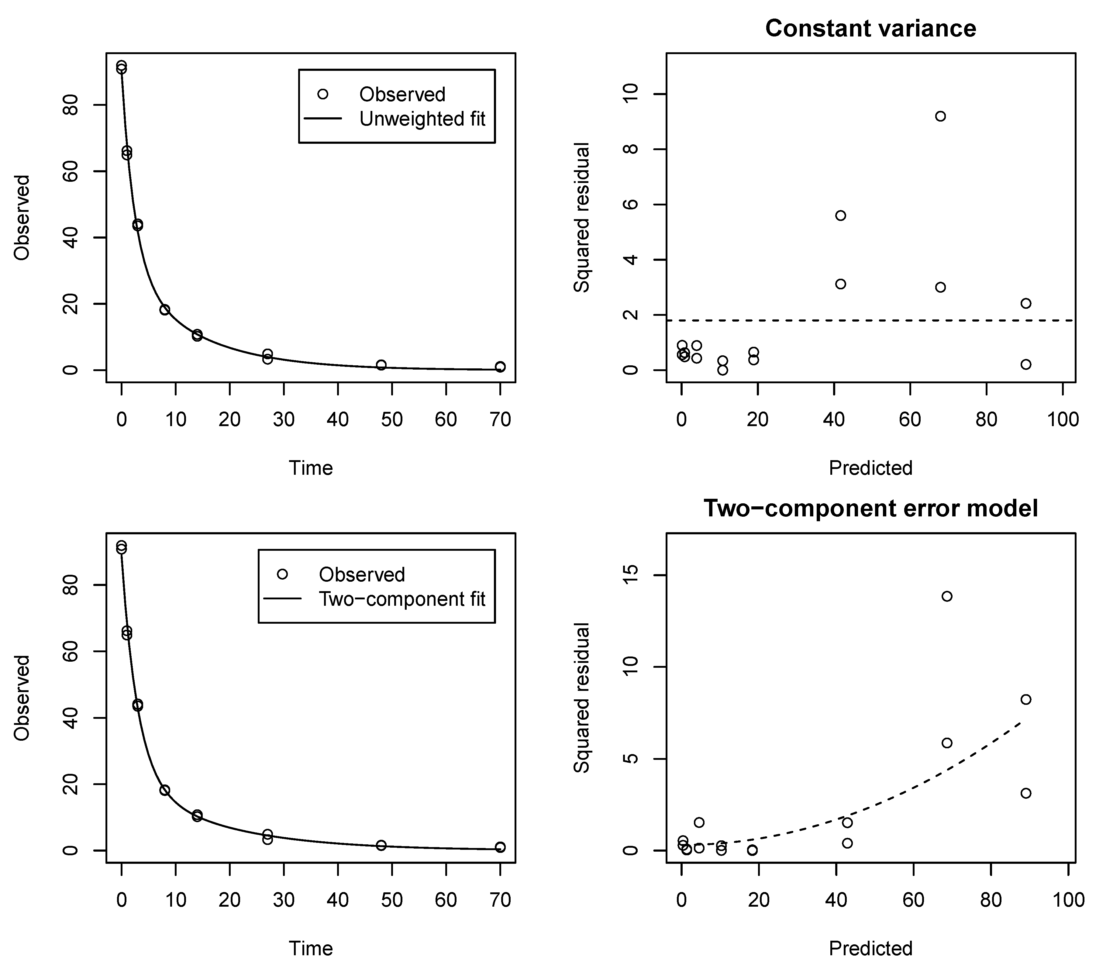
A graphical illustration of the fits and the error structures for Soil Dataset 8, where the improvement of the AIC by using the two-component error model was most pronounced, is shown in
Figure 1. The plots of the squared residuals against predicted values in the two panels to the right illustrate that there was indeed a trend in squared residuals to increase with predicted values and that this trend was adequately reflected by the two-component error model.
3.3. Coupled Fits
Similar observations could be made when simultaneous evaluations of parent decline and metabolite formation and decline were made with a coupled model. For each of the eleven soil datasets featuring one or more metabolites, a parent decline model (either SFO or DFOP) was selected for the parent compound, based on the parent only fits discussed above and coupled to simple first-order (SFO) degradation of the metabolite. The selected coupled models were then fitted using OLS fitting, the variance by variable model, and the two-component error model. The AIC values obtained in these coupled fits are listed in
Table 3.
Only in two cases, ordinary least squares fitting provided the lowest AIC value. The variance by variable error model led to the lowest AIC for four of the datasets. In the remaining five cases, the two-component error model gave the lowest AIC, indicating that the error structure was most adequately represented by this error model.
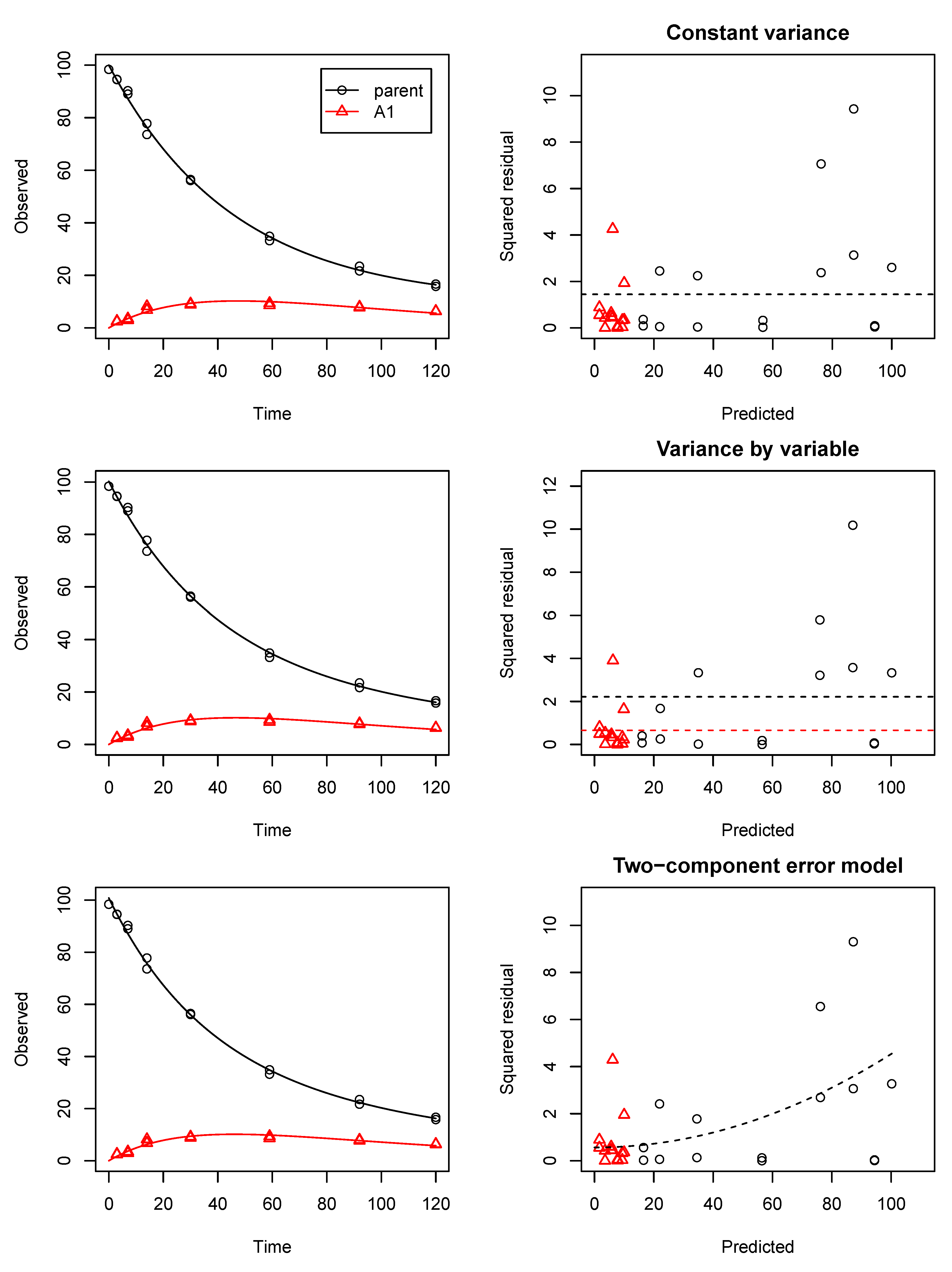
Figure 2 shows the three fits including the three error models for Soil Dataset 3, which was one of the datasets for which the two-component error model provided the lowest AIC. The panels to the right showed that the level of squared residuals was generally lower for metabolite A1, which was the reason why the variance by variable error model gave a lower AIC than the OLS fit assuming the same variance for both compounds. However, it was also visible that there was an increasing trend of the squared residuals with increasing fitted values, which can be described by the two-component error model. These plots suggested that the squared residuals for metabolite A1 were lower than for the parent compound because the residue levels of A1 were lower than the parent residue levels. In this case, it was more efficient to assume that the error depended on the magnitude of the observed value than to assume that it depended on the type of compound observed.
The corresponding degradation model parameters with the
p-values for the
t-test for significant difference from zero are given in
Table 4. While the value for the degradation rate constant
k_A1 for metabolite A1 was nearly the same for all three fits, an interesting observation could be made for the rate constant
k2 for the second phase of the biphasic decline of the parent compound. While in the OLS fit, it had a very low value of 1.2e-5 per day and would not be deemed significantly different from zero, it took on an appreciable value of about 0.007 per day when the variance by variable error model was used. While the
p-value was still far from the usual significance trigger of 0.05 using variance by variable, it dropped to 0.04 if the two-component error model was used, and the estimate for
k2 rose to around 0.008 per day.
This suggests that where the error structure of parent and metabolites was well described by the two-component error model, even the kinetic parameters for the parent compound could be described with greater certainty compared to fitting without metabolite data or compared to fitting with the two other error models available in mkin.
4. Conclusions
The technical feasibility of using alternative error models for the kinetic evaluation of chemical degradation data was demonstrated. A two-component error model derived from experience gathered in analytical chemistry was proposed as a valid alternative to unweighted least squares fitting and to the variance by variable approach commonly used in iteratively reweighted least squares fitting for datasets including transformation products.
For reliable fitting of the components of the two-component error model while optimizing the degradation model parameters, it was found necessary to combine direct optimization of the likelihood function with a three-step procedure, consisting of an unweighted least squares fit to obtain degradation model parameters, a separate optimization of error model parameters with fixed degradation model parameters, and a final optimization of all parameters.
The AIC proved to be valuable for comparison of the error models, but also for comparison of the different degradation models and their combinations with the available error models.
For parent decline datasets and for datasets containing data for the parent and one or two metabolites, the two-component error model provided the most adequate representation of the data based on the AIC in one third of the cases or more.
In one case, a degradation model parameter was even significantly different from zero when using the two-component error model, while the parameter was not significantly different from zero under the other two error models.
In spite of the limited experience with the two-component error model, the results shown in this contribution suggested that it was a valid alternative to the error models used so far. However, it cannot be excluded that assessments will become more conservative if the method will be routinely applied.


