Modelling of Urban Near-Road Atmospheric PM Concentrations Using an Artificial Neural Network Approach with Acoustic Data Input

Abstract

Air quality assessment is an important task for local authorities due to several adverse health effects that are associated with exposure to e.g., urban particle concentrations throughout the world. Based on the consumption of costs and time related to the experimental works required for standardized measurements of particle concentration in the atmosphere, other methods such as modelling arise as integrative options, on condition that model performance reaches certain quality standards. This study presents an Artificial Neural Network (ANN) approach to predict atmospheric concentrations of particle mass considering particles with an aerodynamic diameter of 0.25–1 μm (PM_(0.25–1)), 0.25–2.5 μm (PM_(0.25–2.5)), 0.25–10 μm (PM_(0.25–10)) as well as particle number concentrations of particles with an aerodynamic diameter of 0.25–2.5 μm (PNC_(0.25–2.5)). ANN model input variables were defined using data of local sound measurements, concentrations of background particle transport and standard meteorological data. A methodology including input variable selection, data splitting and an evaluation of their performance is proposed. The ANN models were developed and tested by the use of a data set that was collected in a street canyon. The ANN models were applied furthermore to a research site featuring an inner-city park to test the ability of the approach to gather spatial information of aerosol concentrations. It was observed that ANN model predictions of PM_(0.25–10) and PNC_(0.25–2.5) within the street canyon case as well as predictions of PM_(0.25–2.5), PM_(0.25–10) and PNC_(0.25–2.5) within the case study of the park area show good agreement to observations and meet quality standards proposed by the European Commission regarding mean value prediction. Results indicate that the ANN models proposed can be a fairly accurate tool for assessment in predicting particle concentrations not only in time but also in space.

1. Introduction

Exposure to both particles and noise is associated with an enhanced risk of various adverse health effects [1,2]. Inside urban areas various particle sources can be found [3]. Still, motor traffic is the major source for increased intra-urban levels of particulate matter (PM) inside cities considering low industrial activity [4,5,6]. Furthermore, PM concentrations are highly influenced by background particle transport besides the interference with motor traffic [7]. High noise levels in urban areas are often attributable to local road traffic as well. In Europe, high levels of both noise and particle concentrations mostly occur within street canyons [8].

Numerous studies have evaluated the relation between particle concentrations and noise levels in cities near road arterials assuming that both can be allocated to the same motor traffic emitter. Generally speaking, a relation could be proved between particle concentrations and noise levels; however, the statistical correlation between both is complex and different for various metrics [9]. Recent studies highlight that the correlation between equivalent sound pressure levels (A-weighted or non-weighted) and aerosol concentrations is generally higher for either small particle fractions like PM₁ [10] or ultrafine particle metrics like the particle number concentration (PNC), respectively [7,11,12,13,14]. The correlation tends to increase with decreasing particle sizes [13]. The relation to noise is less strong for coarse particle fractions like PM₁₀ [15] or PM_2.5 [12,14]. The metric of A-weighted equivalent sound pressure levels (SPL_eq(A)) is of particular interest when it comes to the investigation of stressors for humans since SPL_eq(A) is a reference metric that emphasizes the human perception of noise integrated over the entire frequency spectrum. It is, therefore, highly popular in studies where noise levels have been compared to particle concentrations [13]. The metric of SPL_eq(A), however, accentuates by definition frequency ranges around 1 KHz but plays down lower frequency ranges, where most of the sonic energy transport can be expected from motor traffic-induced sounds [16]. Additionally, besides motor traffic sound that can be assigned to sources of particle emissions, many supplementary sources of sound can be found. Until now, only very occasionally optimization of the acoustic data towards an exhausting representative of motor traffic sounds out of the unweighted noise spectrum has been come into focus when evaluated against concentrations of pollutants like PM [13].

Monitoring of particle concentrations with reference methods is an important task due to the surveillance of air quality standards. However, reference sensors are expensive and therefore in Europe mostly very limited measurements are taken inside urban areas. As a result, spatially resolving information on the local urban concentration of e.g., PM is scarce. Recently developed economic micro-sensors have until now not been able to mitigate the poor availability of information in the dimension of space since this generation of micro-sensor platforms still shows mostly poor performance in particular for PM [17].

Modelling approaches can help to address these shortcomings as alternative or supplementary options to instrumental monitoring. Many different approaches have been developed over time. Deterministic models up to full numerical solutions describing the physical phenomena that determine the transportation of pollutants in the atmosphere are powerful approaches to predict concentrations and the distribution of pollutants in time and space [18,19]. Deterministic models were found to be valid methods; but still, there is room for improvement with regard to their performance. Dispersion models can show unacceptable uncertainties despite of the integration of complex physical relationships and vast computational effort that is needed to derive the results (e.g., [20]). Furthermore, for practical applications often crucial input parameters such as local meteorological data and emission rates of pollutants to initiate deterministic models do not exist in reasonable quality or are available only to a limited extent in dimensions of both space and time.

Statistical modelling, as an alternative modelling approach, can be considered an objective estimation technique in the sense that the method is based on statistical data analysis establishing empirical relationships between ambient pollutant concentrations and influencing variables like e.g., meteorological parameters [21,22] or land use patterns [23,24]. The problem is that many common solutions like regression modelling are not applicable for non-linear problems often found in the real world (environmental or ecological contexts). The relationship between e.g., meteorology and pollutant concentrations, in particular, is complex and potentially multi-scale in nature [25]. The same holds true for the conjunction between sound and pollution levels [13]. Beyond, particle concentrations are more prone to changes introduced by micrometeorology; whereas the influence of meteorology on sound propagation is less strong [7,13]. These settings make the complex nature of the problem highly suitable for an artificial neural network (ANN) approach [26]. The ability of ANNs to learn underlying data generating processes without the requirement of prior knowledge of the nature of relationships between variables, given sufficient data samples, has led to popular usage for e.g., the prediction and forecasting in environmental studies, among others [25,27]. ANNs are powerful tools that were successfully developed and tested also for prediction within the field of air quality [26]. ANNs were applied and refined over time for e.g., the prediction of hourly concentrations of NO_x and NO₂ in urban air [28], daily average PM₁₀ concentrations one day in advance [29], hourly concentrations of CO, NO₂, PM₁₀ and O₃ using traffic counts as a major input parameter [30] and ambient air levels of arsenic, nickel, cadmium and lead [22].

In this study, an artificial neural network approach is presented using available meteorological data and inexpensive sound measures as input variables as a cost-effective integrative option to predict aerosol concentrations in urban areas on a basis of 10-min averages where permanent sensor operation is not possible or feasible. The term “prediction” is used hereinafter as a synonym for “now-casting” instead of forecasting establishing the relationship between observed independent variables (e.g., meteorological or acoustical variables) and an observed dependent variable (particle concentrations). Particular concern is put on the selection of input variables, i.e., on the sound data processing in order to determine the sound metric with the maximum predictive information to represent the motor traffic-induced particle emission input of the developed ANN models. The models were developed, validated and tested in a case study environment of a street canyon in direct vicinity to a road arterial (“Aachen-Karlsgraben” test case). In a second step, the validated ANN models were applied and tested by the use of a data set collected within a second research site representing an open green area (“Münster-Aasee” test case). Here the approach was to test for the first time the ability of the ANN approach to gather spatial information on particle concentrations apart from direct vicinity to traffic lanes.

2. Materials and Methods

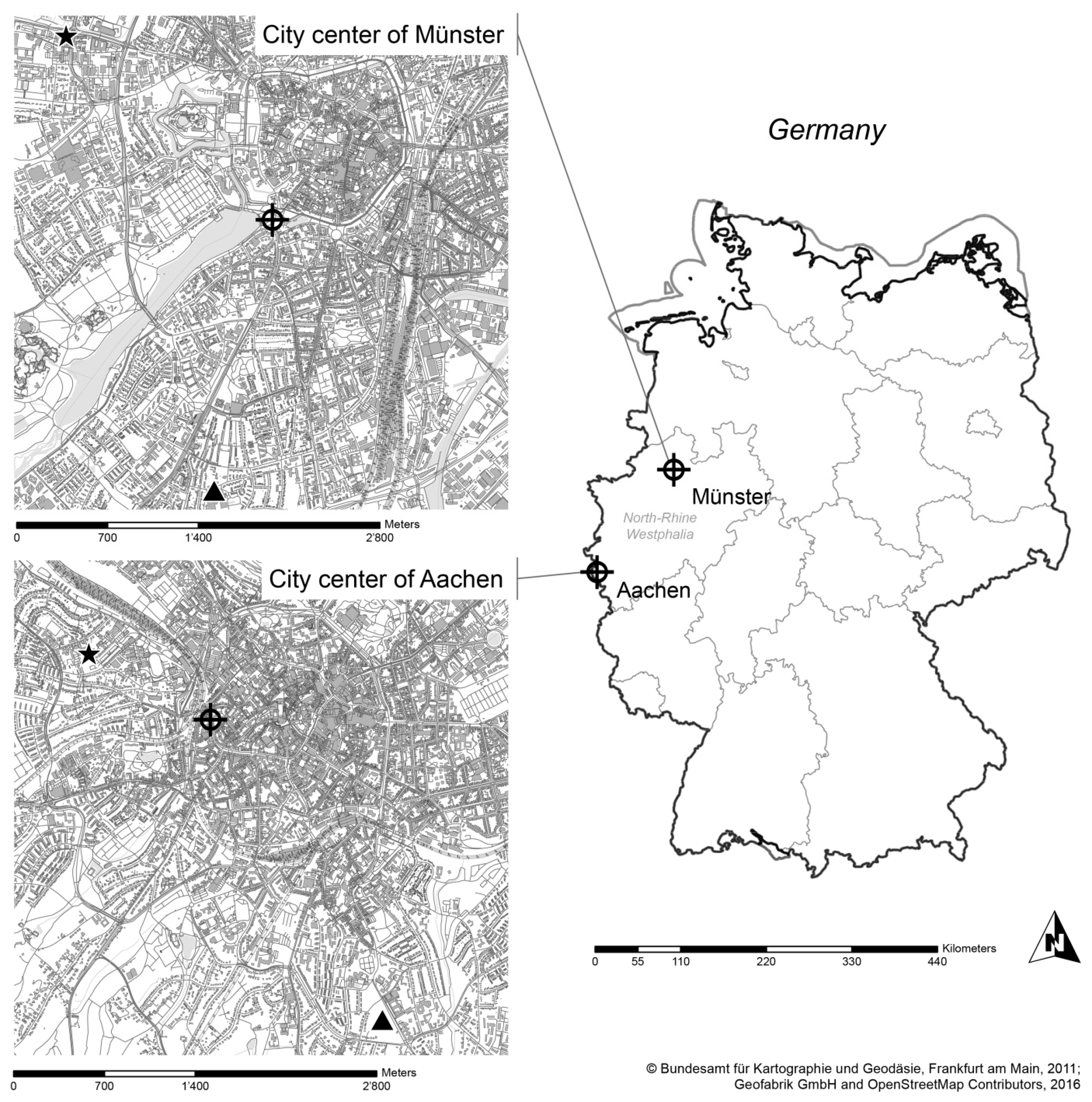
2.1. Research Sites

2.1.1. Aachen-Karlsgraben

The development and the validation of the proposed ANN model approach took place with a dataset that was collected in a typical street canyon, at the most inner circular road named “Karlsgraben” that surrounds the historic district in the West of the city of Aachen, Germany (see Figure 1). Buildings that enclose the street canyon are containing 4–5 floors and major parts of the buildings are of residential use. Only very occasional business is characterizing the research site containing an electronic hardware store as well as two restaurants. The two restaurants feature enclosed dining areas with the kitchens lying backwards of the houses so that in consequence exhaust air containing particles due to cooking, etc. are emitted to the backyard and not into the street canyon under investigation. Both are located on the other side of the road, 30 m beeline from the installed measurement equipment. The building-height(h)-to-street-width(w) aspect ratio of the street canyon h/w is ~1. The “Karlsgraben” road is a loop arterial oriented to North-South direction in the area under study with two traffic lanes (2-way) and an average traffic volume of approximately 501 vehicles per hour daytime, composed of 93% passenger cars, 2% busses (diesel), 4% delivery vehicles and 1% mostly diesel-powered heavy duty vehicles (manually counted for seven randomly picked hours at different times of day during the period of investigation). Besides the larger traffic share of busses at the study site, the composition of traffic there is similar to the average traffic composition in the state North Rhine Westphalia (NRW). According to the German Federal Office for Motor Traffic (Kraftfahrtbundesamt), the overall vehicle fleet composition in 2012 in the state NRW, where the city of Aachen belongs to, was 94% passenger cars (about 30% diesel), 4% delivery vehicles, 2% heavy duty vehicles, and 0.1% busses [31].

The stretch of road under study covers a range of 200 m and is located between two intersections that are controlled with traffic lights. The “Karlsgraben” road features a speed limit of 50 km·h⁻¹; however, because most of the motor traffic is between accelerating and slowing down due to the traffic lights up front and at the end of the stretch of road under study, the average speed of motor traffic was estimated to be ~ 30 km·h⁻¹ (mostly fluent) in front of the data collecting sensors. Field data collection for the “Aachen-Karlsgraben” campaign took place halfway between two traffic lights eastward next to the traffic lane (1 m off-street) curbside of “Karlsgraben” road (see Figure 2).

2.1.2. Münster-Aasee

An open space in the city of Münster, NRW, Germany was used as a test case for the development of the ANN models to examine the performance beyond the bounds of an isolated street canyon. The area under study in Münster is characterized by an inner-city park area with a dimension of 250 m by 350 m. The area under study is featuring “complex terrain”. In this study, “complex terrain” is referred to the complex urban geometry that is characterized by numerous obstacles like houses and vegetation elements with varying height as well as varying ground levels. The site is remote from industrial areas and contains two lakes. The green area is surrounded by isolated freestanding buildings. Four roads are cutting though the park area in Münster where measurements of sound and particle concentrations were taken. One major traffic arterial, “Weselerstrasse”, is oriented from North-East to South-West and contains four traffic lanes (2-way) and an average traffic volume of 2175 vehicles per hour daytime. Field data collection for the “Münster-Aasee” campaign took place at three different locations. One measurement location was in vicinity to the main traffic arterial “Weselerstrasse” (westward, 10 m off-street), where one-third of the data set was collected. Two further locations where data collection took place were located 100 m beeline from “Weselerstrasse” inside the green area eastwards and westwards, respectively. At both measurement locations inside the green area one-third of the complete data set was collected each. Further details of information on the topography of the research site “Münster-Aasee” and the respective collection of data can also be found in [20].

2.2. Artificial Neural Network Approach

Artificial neural network models are universal approximators with the ability to generalize through learning non-linear relationships between provided variables of input(s) and output(s) [32]. The objective of all ANN prediction models is to find an unknown functional relationship $f\left(X,W\right)$ which links the input vectors in $X$ to the output vectors in $Y$ [25]. All ANN models are basing on the following form described with the equation (Equation (1)) given by [33]:

$$Y=f\left(X,W\right)+\mathsf{\epsilon }$$

(1)

where $W$ is the vector of model parameters (connection weights) and $\mathsf{\epsilon }$ represents the vector of model errors. Thus, in order to develop the ANN model, the vector of model inputs ($X$), the form of the functional relationship ($f\left(X,W\right)$), which is governed by the network architecture and the model structure (e.g., the number of hidden layers, number of neurons and type of transfer function) and the vector of model parameters ($W$), which includes the connection and bias weights, have to be defined [33]. The development of the ANN models for the different test cases in this study followed the guidelines and recommendations on ANN model development published in the reviews from [25,27,33] where applicable. Developing of the ANN model in this study was realized using “neuralnet 1.33” with the R software package, version 3.3.1 [34].

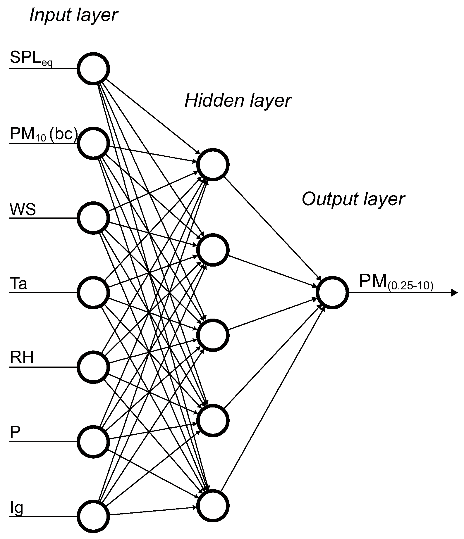
2.2.1. Model Architecture—Multi-Layer Perceptron

A Multi-Layer Perceptron (MLP) was selected as the basis of the ANN models in this study to predict mass concentrations of particles with an aerodynamic diameter (DAE) between 0.25 μm and 1 μm (PM_(0.25–1)), between 0.25 μm and 2.5 μm (PM_(0.25–2.5)), between 0.25 μm and 10 μm (PM_(0.25–10)) as well as particle number concentrations with a DAE between 0.25 μm and 2.5 μm (PNC_(0.25–2.5)). The MLP is the most commonly used ANN model architecture [33,35] and has been found to perform well for applications like the prediction of air pollutant concentrations [26,30]. MLPs typically contain three types of layers of neurons: the input layer, the hidden layer(s), and the output layer [33]. As feed-forward networks, MLPs propagate information only in one direction, i.e., from the input layer to the output layer. In this study, an MLP containing three single layers (one input layer, one hidden layer, one output layer) was used for all ANN models developed (see Figure 3). The number of input neurons (IL_n) is determined by the selected number of input variables. The output layer (OL) in each ANN model is restricted to a single output neuron, i.e., the variable that will be predicted (in this study either PM_(0.25–1), PM_(0.25–2.5), PM_(0.25–10) or PNC_(0.25–2.5)). The number of neurons in the hidden layer (HL_n) has to be determined in the model structure selection process. The neurons of the MLP are inter-connected by weights and output signals which are a function of the sum of the inputs to the neuron modified by a transfer function [25]. Both linear and non-linear transfer functions can be used at hidden and output layers [27]. Various types of functions are possible. However, ANN models where inputs are summed and processed by a non-linear function have the ability to represent any smooth measurable function between the input and output vectors, and are therefore highly suitable to capture complexity and non-linear relationships inherent in the systems being modeled [33]. The suitable set of weights is found through training (finding the weight with the smallest error) of the ANN model with a subset of the sample that represents the input and output vectors [36]. Different training algorithms can be applied to minimize the error function.

2.2.2. Input Variable Selection

Input variable selection is one of the most important steps in ANN model development [33]. An appropriate set of ANN model inputs “is considered to be the smallest set of input variables required to adequately describe the observed behavior of the system” [37]. Hence, the input selection process was divided in two different actions to determine an appropriate set of inputs. In a first step, input significance is justified using an ad hoc approach where potential input variables (i.e., candidates) were determined basing on a priori knowledge considering the nature of the problem and available data. When it comes to the prediction of local aerosol concentrations as part of the urban roughness layer two main aspects need to be considered: sources of particles and characteristics of particle dispersion [30]. Motor traffic emissions regarding both the amount of combustion processes and blown up dust as well as tire and break abrasions are identified to be the major source of particles near urban arterials [4,6,38]. Vehicular emissions are related to the volume of traffic, vehicle type and speed [30], which, in turn, are assumed to be attributable to traffic sound. A linear and well established correlation between traffic counts and sound levels could be proved [13,39]. Therefore, time integrals of equivalent sound pressure levels were considered as input variable candidates representing the source of particles inside the ANN model. Overall, 24 candidates of different sound metrics were considered (for details, see below Section 2.3.2). Local concentrations of particles are furthermore influenced by the source of background particle transport [7]. In consequence, a second input variable serving as another representative of particle sources inside urban areas was defined using 24-h moving averages of the PM₁₀ background concentration (PM₁₀ (bc)) obtained from suburban government stations. Considering the variation of pollutant transportation, i.e., the particle dispersion, it is assumed that meteorological conditions are the major factors influencing these dynamics [13]. Variables of atmospheric air temperature (Ta) and pressure (P), relative humidity (RH), wind speed (WS), wind direction (WD) and global radiation (Ig) are directly or indirectly associated with variations of particle transportation [30,40,41] and were consequently considered as meteorological input variable candidates in the development of the ANN models. As an addition, all of the considered meteorological variable candidates are routine metrics that are available at almost every meteorological station and available at low additional costs. Precipitation is also proved to have a major impact on both particle concentrations due to wash-out effects [42] and sound emissions of motor traffic mainly due to shifted tire sound characteristics [43]. However, precipitation was deliberately left out of consideration in this study to keep the nature of the problem for the development process of the ANN model as simple as possible.

Input variables need to be determined based on both the significance and independence of inputs [27]. Consequently, an analysis of Partial Mutual Information (PMI) was applied to proof relevance and independency of the proposed initial candidate set of acoustical and meteorological variables determined during the ad hoc selection step. The PMI algorithm was selected over other commonly used methods such as generalized linear models (GLMs), as it is proved to be a superior approach in particular to examine non-linear dependences [44]. More information on the mathematical basis of the PMI analysis can be found in [37,45]. The goal was to sample out a set of variables with maximum predictive power and minimum redundancy since redundant information in the model input stage can cause various problems; one of the most important being the likelihood of overfitting as a result of confusion during the training process of the ANN model [33,36]. The final input selection using PMI was justified using the Akaike Information Criterion (AIC), which is a measure of the trade-off between ANN model complexity and the information within the candidate set of inputs, as a function of the number of input candidates. The AIC is the recommended criterion within the use of PMI for samples where the distribution of data may be unknown and the assumption of Gaussian distribution may not hold [37]. Variable candidates have been selected in an iterative process up until a minimum AIC was reached for a given set of variable candidates which represents the optimum number of inputs to be selected [37]. For reasons of comparison all ANN models have been developed additionally without using acoustic data input. Calculated AICs for individual input variable selection steps as well as the input variables defined for the optimum model architecture of each ANN model are presented below in Section 2.2.4.

2.2.3. Data Splitting

The valid data set, including the selected input (see Section 2.2.2) and output variables, were divided into training, validation and testing subsets, in order that cross-validation could be used to avoid overfitting of the MLP and to ensure best possible generalization of the ANN model on unknown input data. The sample was divided into data subsets with a split-sample-ratio of 70% training data to 20% validation data to 10% test data. One popular approach to split the sample in different subsets is to assign data points according to the random principle. While this may be an adequate method for large sample sizes there is a chance that the data in one of the subsets may be biased towards extreme or uncommon events [25]. In this study, a method based on stratified sampling of the Self-Organizing Map (SOM) was used to split the data set into subsamples ensuring that the statistical properties of the subsets are similar [46]. In principle, a SOM clusters the available data by delineation of sub-domains within a dataset for which data within the same sub-domain are similar, but distinct from data in other sub-domains. Stratified random·sampling is applied to allocate data samples from each SOM cluster to the subsets of training, validation and testing. As a result, it is made certain that patterns from all identified sub-domains of the multivariate input-output space are represented in each subset [46]. The training set consists of data vectors used for training the network, i.e., fitting the weights of the neurons of each layer for the desired output. The subset of validation data was used to tune the ANN model structure. The test set was used to assess the performance of the developed ANN model after training on unseen input data. SOM-based stratified data splitting (SBSS) was performed following the recommendations of [46] regarding the settings of the SOM. The adjustment of the SOM map units is one of the most influential parameters and depends on the SOM grid size (SOM_gs) which should be determined by the sample size of the data set (s_n), where SOM_gs should be equal to ~s_n^0.54. The length of the SOM map should be 1.6 times the SOM_gs, whereas the width should be equal to the SOM_gs, resulting in a SOM map size used in this study of a ratio of 5.8 by 3.6 within the “Aachen-Karlsgraben” test case and a ratio of 4.3 by 2.7 within the “Münster-Aasee” test case representing the length and width respectively. Proportional random sampling has been applied to the sample. SOM parameters that have been used for implementing SBSS are presented in

Table 1. Self-Organizing Map (SOM) parameters for implementing SOM-based stratified data splitting (SBSS). “Münster-Aasee” test case settings are given in brackets if distinct from “Aachen-Karlsgraben” test case settings.

Parameter	Ordering	Tuning
Initial learning rate	0.9	0.1
Initial neighborhood size	3.6 (2.7)	1
Epochs	2	20

.

In Figure 4 data histograms for both test cases and all ANN models of the trained SOMs and data sets of input variables are shown illustrating how input data vectors are clustered by the SOM. The data histogram visualization shows how many vectors were assigned to each cluster. More detailed mathematical descriptions regarding SOM-based stratified sampling can be found in [46].

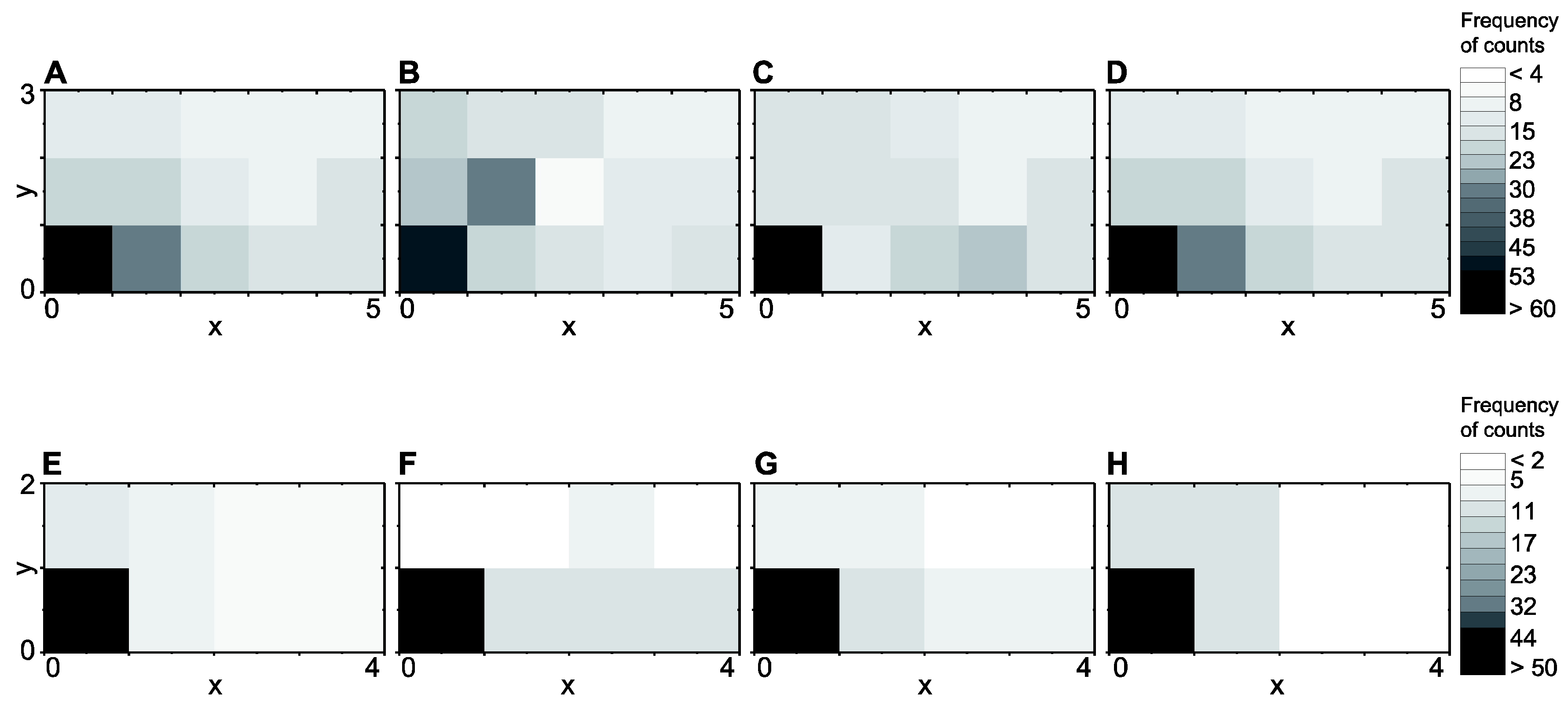
2.2.4. Model Structure Selection

Together with the ANN model architecture, the model structure defines the functional relationship $f\left(X,W\right)$ between model inputs and outputs (Section 2.1, Equation (1)). Model structure selection includes the determination of the optimum number of neurons in the hidden layer and how they process incoming signals by the use of suitable transfer functions [46]. In general, an optimum ANN model structure minimizes the uncertainty of the network and maximizes model parsimony considering network size [27]. The model structure can be determined by the use of a stepwise iterative process which is the most-used systematical application to find out the optimal number of neurons in the hidden layer [33]. In a first model structure selection step, a constructive algorithm was applied in the ANN model development process. The iterative procedure started by using the defined IL_n-HL_n-OL architecture of the ANN model (Section 2.2.1; Section 2.2.2), combined with the simplest ANN model structure possible (HL_n = 1). The network structure was gradually made more complex by adding neurons in the hidden layer, one at a time, until there was no significant improvement in model performance. Since it is recommended that the ratio of the number of data points used for training to the number of the network weight and biases should be always greater than 2.0 [47] the network size was kept reasonable in size according to the sizes of the data samples (see below Section 2.3). The ANN model structure was tested on the basis of the Root Mean Squared Error (RMSE) of the network (see below, Section 2.5). The second part of this optimization process is the determination of the best suitable transfer function. Two different non-linear variants of functions were considered in the development process of the ANN model, i.e., hyperbolic tangent and the logistic sigmoidal. The obtained RMSEs for different ANN model structures created during the refinement process, considering both different number of neurons in the hidden layer and two different transfer functions, are presented in Figure 5. It turned out that the best performing final ANN model to predict PM_(0.25–10)-concentrations was operated by using a logistic sigmoidal transfer function. The best performing ANN models to predict concentrations of PM_(0.25–1), PM_(0.25–2.5) and PNC_(0.25–2.5) were using a hyperbolic tangent transfer function. The optimum HL_n to predict concentrations of PM_(0.25–1) was found to be six. The best performing ANN model to predict concentrations of PM_(0.25–2.5) contained four hidden neurons. The optimum HL_n of the ANN models to predict concentrations of PM_(0.25–10) and PNC_(0.25–2.5) were detected to be five (see Figure 5). The ANN models using only input data of meteorology and background particle transport developed for comparison passed the same procedure of model structure selection as described above. A summary of the finalized ANN model architecture used to predict concentrations of PM_(0.25–1), PM_(0.25–2.5), PM_(0.25–10) and PNC_(0.25–2.5), including the determined number of neurons in the input layer, their respective input variables as well as the HL_n and the best performing transfer functions, is presented in

Table 2. Summary of the finalized Artificial Neural Network (ANN) model architecture including number of neurons in the input layer (IL_n) input variable candidates (IVC) and respective Akaike Information Criterion (AIC) values given in square brackets, number of neurons in the hidden layer (HL_n), determined transfer functions and the dedicated output layer (OL). Numbers in parentheses indicate settings used for the alternative models using input variables excluding acoustic data. Determined input variables for the final ANN models are indicated in bold letters.

ILn	5 (4)	6 (5)	6 (5)	7 (6)
IVC [AIC]	PM10 (bc)	PM10 (bc)	PM10 (bc)	PM10 (bc)
	Ta [−428]	RH [−242]	RH [−171]	RH [−241]
	P [−843]	Ta [−274]	Ta [−235]	Ta [−283]
	Ig [−868]	Ig [−358]	WS [−251]	Ig [−365]
	WS [−866]	P [−366]	P [−270 ]	WS [−423]
	WD [−832]	WS [−346]	WD [−246]	P [−430]
	RH [−810]	WD[−388]	Ig [−210]	WD [−421]
	SPLeq [−6]	SPLeq [−8]	SPLeq [−10]	SPLeq [−9]
	SPLeq15Hz(A) [−1]	SPLeq15Hz [−2]	SPLeq15Hz [−1]	SPLeq15Hz(A) [−4]
	SPLeq16kHz [23]	SPLeq34Hz [10]	SPLeq15Hz(A) [2]	SPLeq15Hz(A) [5]
	SPLeq63Hz(A) [51]	SPLeq34Hz(A) [14]	SPLeq63Hz(A) [27]	SPLeq34Hz [8]
	SPLeq15Hz [55]	SPLeq15Hz(A) [18]	SPLeq125Hz(A) [55]	SPLeq34Hz(A) [10]
	SPLeq34Hz(A) [70]	SPLeq16kHz [45]	SPLeq34Hz [70]	SPLeq250Hz(A) [14]
	SPLeq16kHz(A) [78]	SPLeq250Hz(A) [61]	SPLeq16kHz(A) [127]	SPLeq250Hz [19]
	SPLeq125Hz(A) [112]	SPLeq250Hz [66]	SPLeq8kHz [154]	SPLeq16kHz(A) [57]
	SPLeq8kHz [137]	SPLeq16kHz(A) [83]	SPLeq250Hz(A) [168]	SPLeq16kHz [73]
	SPLeq250Hz(A) [154]	SPLeq63Hz(A) [117]	SPLeq34Hz(A) [176]	SPLeq63Hz(A) [105]
	SPLeq63Hz [165]	SPLeq125Hz(A) [147]	SPLeq16kHz [189]	SPLeq125Hz(A) [133]
	SPLeq34Hz [174]	SPLeq8kHz [171]	SPLeq63Hz [201]	SPLeq63Hz [146]
	SPLeq125Hz [189]	SPLeq63Hz [183]	SPLeq8kHz(A) [207]	SPLeq125Hz [161]
	SPLeq250Hz [194]	SPLeq125Hz [199]	SPLeq125Hz [225]	SPLeq8kHz [184]
	SPLeq8kHz(A) [200]	SPLeq8kHz(A) [205]	SPLeq250Hz [229]	SPLeq8kHz(A) [189]
	SPLeq500Hz(A) [207]	SPLeq500Hz [212]	SPLeq4kHz(A) [241]	SPLeq500Hz [195]
	SPLeq4kHz [219]	SPLeq4kHz(A) [224]	SPLeq500Hz [247]	SPLeq4kHz [208]
	SPLeq1kHz [221]	SPLeq1kHz [225]	SPLeq500Hz(A) [250]	SPLeq1kHz [210]
	SPLeq4kHz(A) [226]	SPLeq4kHz [230]	SPLeq4kHz [253]	SPLeq4kHz(A) [215]
	SPLeq500Hz [230]	SPLeq500Hz(A) [233]	SPLeq2kHz(A) [257]	SPLeq500Hz(A) [218]
	SPLeq(A) [240]	SPLeq(A) [243]	SPLeq(A) [260]	SPLeq(A) [233]
HLn	6 (7)	4 (3)	5 (4)	5 (4)
Transfer function	Hyp-Tan	Hyp-Tan	Log-Sig	Hyp-Tan
	(Hyp-Tan)	(Hyp-Tan)	(Log-Sig)	(Hyp-Tan)
OL	PM(0.25–1)	PM(0.25–2.5)	PM(0.25–10)	PNC(0.25–2.5)

.

2.2.5. Model Calibration—Backpropagation Algorithm

The process of finding a set of connection weights between neurons that results in an ANN model with a given functional form to best represent the desired input/output relationship is called “training” [33]. The back-propagation (BP) algorithm, a first-order local search procedure, is the most used algorithm for training an MLP [25]. The learning process basically consists of two iterative steps: forward computing of data and backward propagation of error signals [30]. Developed by [48], BP uses a gradient descent algorithm in which the network weights are moved along the negative of the gradient of the performance function [36].Usually, the BP algorithm is implemented following the steps hereinafter: (I) Initialization of network weights starting with small random values; (II) Propagation of an input vector from the training subset of data through the network to obtain an output; (III) Calculation of an error signal; (IV) Back-propagation of the error signal through the network; (V) Weight-adjustment at each neuron to minimize the overall error; (VI) Repetition of steps II–V with the next input vector, until the overall error is satisfactorily small [25]. Training was stopped when the performance of the MLP on the test sample reached a maximum, which, in turn, was assumed to represent the global minimum of the error surface. Details of the mathematical formulation of the BP algorithm can be found in [49].

2.3. Field Data—Collection and Pre-Processing

All simultaneously conducted measurements in Aachen, including the collection of aerosol data, acoustics and meteorology were taken at different days of week and different times of day for the reason that the dataset represents a best possible spectrum of both noise levels and particle concentration levels representative for the area under study during daytime at business days. Data collection at the “Aachen-Karlsgraben” research site took place at 27 October 2016, 28 October 2016, 3 November 2016, 4 November 2016 and 30 November 2016 at different times of day between 04:30 a.m. at the earliest and 08:00 p.m. at the latest resulting in a sample of overall 293 10-min averages of all variables. Outliers (e.g., due to sounds resulting from ambulance or police sirens) as well as the first and last ten minutes of data recordings were manually deducted from the raw data set. The pre-processed sample used for the development of the ANN models consists of 275 10-min averages of all variables. Meteorological prerequisite conditions for the Aachen campaign were chosen to avoid rainy periods and atmospheric conditions concerning both well-marked dilution of pollutants as well as conditions where resuspension of particles due to gusting wind is likely, i.e., data collection took place during low wind speed conditions and an upstream wind vector perpendicular to the street canyon under study. The measurements in Münster took place at three different weekdays in February as well as three different weekdays in July 2015 between 10:00 a.m. and 05:00 p.m. local time resulting in a pre-processed sample of overall 97 10-min averages of all variables to evaluate the performance of the developed ANN models under different initial conditions beyond an isolated street canyon.

2.3.1. Particles

Local aerosol measurements were carried out using an optical particle counter (OPC), Model EDM 107G (Grimm GmbH, Ainring, Germany) to determine different metrics regarding the concentration of airborne particles. The OPC bases on the approach of single particle counting by the use of light scattering technique. The number of contained particles of the air sample is derived from the frequency of scattered light pulse signals. Particle sizes are obtained from the amplitude of the backscatter signal. The OPC classifies detected particles into a size distribution in a range between 0.25 and 32 μm DAE containing 31 different size channels. Internally, the particle number size distribution is converted into mass concentrations for an indicated average time interval. The sensor operates at a volumetric flow rate of 1.2 L min⁻¹ and a time resolution of 6 s [50]. The OPC used had been factory calibrated on a regular basis (VDE standard 0701-0702) within the calibration validity period and was calibrated last on 13 January 2015. In all cases particles were sampled at the mean respiratory height of 1.6 m agl and stored as 10-min arithmetic means of PM_(0.25–1), PM_(0.25–2.5)), PM_(0.25–10) and PNC_(0.25–2.5). Data of PM₁₀ (bc) were obtained as 24-h moving averages from government air quality sites Aachen-Burtscheid (AABU) and Münster-Geist (MSGE), operated by the North Rhine-Westphalian State Office for Nature, Environment, and Consumer Protection (LANUV) assuming that both government stations represent the urban background particle concentration which can be expected at the research sites even though both government stations are around 2.5 km beeline from respective areas under investigation.

2.3.2. Acoustics

Time series of physical sound pressure values were captured with a mobile recorder (Type H6, Zoom Corporation, Tokyo, Japan) at 44.1 kHz sampling rate with 24 Bit resolution using an omnidirectional microphone (KE-4 electret-microphone, Sennheiser Electronic GmbH & Co. KG, Wedemark, Germany). The calibration process has been performed in a post-processing step by comparing a Root Mean Square (RMS) 1 kHz pure-tone signal at 94 dB re 20 μPa from a portable sound source (Type 4231 Sound Calibrator, Brüel & Kjær Sound & Vibration Measurement A/S, Nærum, Denmark), which has been captured for each measurement time-series individually (once per day). The measurements were carried out with the microphone installed on a tripod 1.2 m agl at the same location where data of particle concentrations were taken (Section 2.3.1). From·sound pressure time series, 10-min averages of equivalent sound pressure levels as integrals over the entire captured bandwidth of frequencies between 0 Hz and 22 kHz (SPL_eq) were determined. Furthermore, 10-min averages of sound pressure levels representing single octave bands of 15 Hz, 34 Hz, 63 Hz, 125 Hz, 250 Hz, 500 Hz, 1 kHz, 2 kHz, 4 kHz, 8 kHz and 16 kHz were calculated. Similarly, equivalent A-weighted sound pressure levels as described by ISO standard 226:2003 were computed as 10-min averages [16] again either as integrals over the captured bandwidth of frequencies between 0 Hz and 22 kHz (SPL_eq(A)) or as metrics of single octave bands as mentioned before. Descriptive statistics concerning the observed aerosol concentrations and acoustic data of both campaigns are summarized in

Table 3. Descriptive statistics concerning arithmetic mean values (AM) and standard deviations (SD) of observed particle concentrations as well as mean values (L_eq) and 10/90% percentiles (L₁₀/L₉₀) of acoustic data of the “Aachen-Karlsgraben” and “Münster-Aasee” test cases.

Variable	PM(0.25–1)	PM(0.25–2.5)	PM(0.25–10)		PNC(0.25–2.5)		SPL
	(μg·m−3)				(#·dm−3)		(dB)
“Aachen-Karlsgraben”	AM: 15.9 SD: 4.2	AM: 19.4 SD: 5.3	AM: 30.4 SD: 8.9		AM: 545 SD: 217		Leq: 74.1 L10: 79.7 L90: 63.4
“Münster-Aasee”	AM: 16.3 SD: 10.2	AM: 18.4 SD: 9.9	AM: 28.7 SD: 9.1		AM: 545 SD: 460		Leq: 69.5 L10: 75.2 L90: 62.0

. Mean values of observed sound levels reflect average values that are published by the state government of NRW for the areas under study. Furthermore, it is stated that at both research sites of the “Aachen-Karlsgraben” and the “Münster-Aasee” campaigns motor traffic is the major source of sound [51].

2.3.3. Meteorology

Meteorological input variables in this study consist of data from nearby weather stations, whose values are monitored in real time by the RWTH Aachen University (6°03′40″ E, 50°46′44″ N; 1500 m beeline from the area under study of “Aachen-Karlsgraben”) and the University of Münster (7°35′45″ E, 51°58′9″ N; 2100 m beeline from the area under study of “Münster-Aasee”), respectively. Meteorological data of local authorities have been chosen in order that they are available at no/low additional costs. Since many cities operate meteorological monitoring stations this approach ensures a low-cost possibility for future applications of the model. In Aachen the wind sensor to determine WD and WS (Wind Monitor 05103, R.M. Young Company, Traverse City, MI, USA) is installed on top of a roof (6.5 m above the rooftop) in 29 m agl. The shielded temperature and humidity sensor (CS215, Campbell Scientific, Inc., Logan, UT, USA) is mounted on a mast in 2 m agl. [52]. During the time of data collection during the campaign in Aachen 2016 the wind was coming from·south-westerly directions (185°–270°), with an average wind speed of 3.2 m·s⁻¹ (in 29 m agl). At the weather station in Münster sensors to determine WD and WS (WindSonic Anemometer RS-232, Gill Instruments Limited, Lymington, Hampshire, UK) as well as the shielded temperature and humidity sensor (41382VC, R.M. Young Company, Traverse City, MI, USA) are mounted on a permanent mast on top of a roof (10 m above the rooftop) in 34 m agl. During the Münster campaign in February 2015 the wind was predominantly coming from easterly directions, with an average wind speed of 4 m·s⁻¹. Varying wind directions but wind mostly coming from northeast and wind speeds between 2 m·s⁻¹ and 5 m·s⁻¹ being most common were observed during the campaign in July 2015. Conditions were dry with no precipitation during the periods of data collection in Münster.

2.4. Field Data—Post-Processing

Before computing, data of both input and output variables were normalized. In this study, data of all variables used were normalized into the range [0, 1] with:

$$X_{norm}=\frac{\left(X_i-X_{min}\right)}{\left(X_{max}-X_{min}\right)}$$

(2)

where $X_{norm}$ is the normalized value, $X_i$ is the original value, and $X_{min}$ and $X_{max}$ are the minimum and maximum values out of the sample of$X_i$. This was due to eliminate the influence of different dimensions of data and to avoid overflows of the ANN model during calculations as a result of very large or small weights towards a maximization of model parsimony considering computational effort [28]. After the computation, output values were transformed back to real prediction data.

2.5. Performance Measures

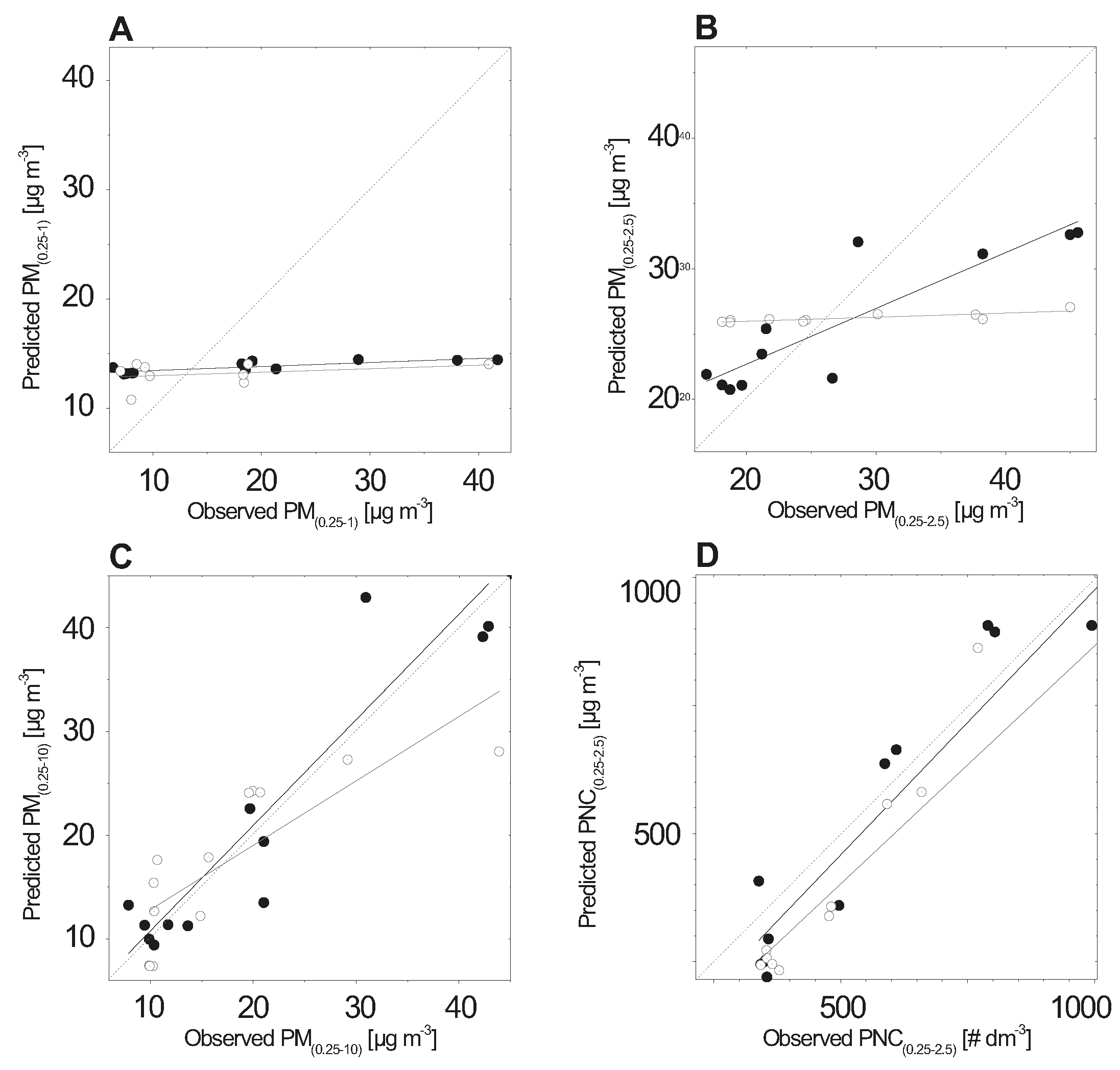
In order to evaluate the performance of the ANN models, several statistical performance indicators were used, namely the RMSE, the Mean Bias (MB), the Centralized Mean Squared Error (CRMSE) the Model Efficiency score (MEF) and the Fractional Bias (FB). The RMSE (Equation (3)) was mainly used in the development process of the ANN model and represents residual errors, which gives a global perspective of the differences between the observed and predicted values [53]:

$$RMSE=\frac{1}{n}\sqrt{{\displaystyle \sum }_{i=1}^n{\left(C_{P_i}-C_{O_i}\right)}^2}$$

(3)

where $C_O$ and $C_p$ are the observed and predicted concentrations, respectively. A graphical approach (target diagram) was used as an additional measure providing an exhaustive indication of model response [54]. The methodology of the target diagram bases on the main principle of [55] and was modified by the Joint Research Centre (JRC) of the European Commission within the framework of the Forum for Air Quality Modelling in Europe (FAIRMODE) to develop a harmonized methodology to evaluate model results based on a consensus set of statistical indicators. The methodology of the target diagram has been introduced by [56] within the DELTA tool. The target diagram reports the MB and CRMSE, both normalized by the standard deviation of the observations (${\sigma }_O$), on the abscissa and ordinate, respectively [54]. The MB is given by Equation (4):

$$MB=\frac{1}{n}{\displaystyle \sum }_{i=1}^n\left(C_{P_i}-C_{O_i}\right)=\overline{C_P}-\overline{C_O}$$

(4)

The CRMSE is described by Equation (5):

$$CRMSE=\frac{1}{n}\sqrt{{\displaystyle \sum }_{i=1}^n{\left[\left(C_{P_i}-\overline{C_P}\right)-\left(C_{O_i}-\overline{C_O}\right)\right]}^2}$$

(5)

The target diagram includes a boundary circle of unit radius that defines the acceptable limit value of the MEF [22]:

$$MEF=1-{\left(\frac{RMSE}{{\sigma }_O}\right)}^2$$

(6)

For an acceptable model, the target value of model results must be plotted inside the boundary circle (radius = 1) of the target diagram, so that the calculated MEF becomes >0 [22]. Moreover, when the requirements of an acceptable model are fulfilled considering MEF, it is automatically guaranteed that predictions and observations are positively correlated. Generally, the closer the reached performance score is to the origin of the target diagram, the better is the model performance [54]. The FB was used as an additional basic measure of model performance. The FB represents a fundamental indicator of discrepancy between the samples of prediction and observation values, respectively [57]. The FB is dimensionless and normalized. Values of the FB range between −2 and +2 for extreme over- or under-prediction of the model, where a value of zero represents a perfect model. The formula is given by Hanna, 1988 (Equation (7)):

$$FB=\frac{2\left({\overline{C}}_O-{\overline{C}}_p\right)}{\left({\overline{C}}_O+{\overline{C}}_p\right)}$$

(7)

3. Results

Four ANN models to predict concentrations of PM_(0.25–1), PM_(0.25–2.5), PM_(0.25–10) and PNC_(0.25–2.5) using input data of SPL_eq, PM₁₀ (bc) as well as meteorological conditions were developed and validated with a data set collected during the campaign “Aachen-Karlsgraben”. Similarly four ANN models were developed excluding input data of acoustic sound for comparison reasons. After individual training of the networks by the use of training data sets taken from the measurement campaigns “Aachen-Karlsgraben” and “Münster-Aasee”, respectively, their predictive performance using unseen test input data concerning 10-min averages were evaluated. For that purpose, ANN model results were compared to observations. The ANN model predictions of the “Aachen-Karlsgraben” test case reveal mixed results in this regard. In Figure 6 10-min averages of predicted PM_(0.25–1), PM_(0.25–2.5), PM_(0.25–10) and PNC_(0.25–2.5) concentrations over respective observations are presented. It can be seen that all predictions are positively related to observations (slope: 0.02–0.24). However, predictions of PM_(0.25–1) and PM_(0.25–2.5) did not coincide to observations (R²: 0.05–0.13). The model to predict concentrations of PM_(0.25–2.5) seems to be almost completely insensitive to model inputs with very little variation within the prediction sample. The relation of model predictions to observations regarding PM_(0.25–10) and PNC_(0.25–2.5) within the “Aachen-Karlsgraben” test case is moderate (R²: 0.28–0.48). In comparison, the ANN models using inputs without acoustic data failed to predict concentrations of PM_(0.25–1) (R²: 0.16, slope: 0.01) and PM_(0.25–10) (R²: 0.14, slope: 0.02). In these cases the models were completely insensitive to inputs. Observations concerning the metric of PNC_(0.25–2.5) were reproduced similarly to results of the ANN model that incorporated the acoustic data input. Depiction B of Figure 6 unveils a better performance for PM_(0.25–2.5) of the ANN model that excluded acoustic data input with a good reproduction of observations (R²: 0.35, slope: 0.81) albeit noticeable scatter within the prediction sample. Figure 7 shows 10-min averages of predicted PM_(0.25–1), PM_(0.25–2.5), PM_(0.25–10) and PNC_(0.25–2.5) concentrations compared to observations calculated with the ANN models using unseen input data of the “Münster-Aasee” test data sets. It becomes obvious that both ANN models with and without the use of acoustic input data were again not able to reproduce measurement data of PM_(0.25–1) (slope: 0.03–0.11). The models were completely insensitive to the inputs indicated by constant predictions values over the entire range of observations with almost no variation in the prediction sample. Concerning PM_(0.25–10) within the “Münster-Aasee” test case it turned out that the ANN model that used additional acoustic data inputs calculated decent predictions (R²: 0.78, slope: 0.43) whereas the ANN model that excluded acoustic data input was again insensitive to input variables (R²: 0.69, slope: 0.03). Results of predicted concentrations of PM_(0.25–2.5) and PNC_(0.25–2.5) of both types of ANN models show a very good agreement to observations over the entire concentration range (R²: 0.65–0.9; slope: 0.62–1.04). The addition of acoustic data to the set of input variables turned out to improve the accuracy of model predictions calculating concentrations of both PM_(0.25–10) and PNC_(0.25–2.5) within the “Münster-Aasee” test cases.

Performance measures as well as statistics concerning the test samples of measurement data are summarized in

Table 4. Artificial Neural Network (ANN) model performance measures and test set statistics including coefficients of determination between the observation and prediction sample (R²) as well as the respective slopes of the regression lines, mean particle concentration values, standard deviations of the observations (SD) and standard deviations of predictions (SD’) of the “Aachen-Karlsgraben” and “Münster-Aasee” test cases, respectively. Values in brackets indicate results derived from alternative ANN models using input variables excluding acoustic data.

OL	“Aachen-Karlsgraben”				“Münster-Aasee”
	PM(0.25–1)	PM(0.25–2.5)	PM(0.25–10)	PNC(0.25–2.5)	PM(0.25–1)	PM(0.25–2.5)	PM(0.25–10)	PNC(0.25–2.5)
RMSE	5.97 (4.27) [μg·m−3]	6.88 (5.09) [μg·m−3]	7.78 (9.35) [μg·m−3]	167 (208) [#·dm−3]	12.29 (10.11) [μg·m−3]	5.71 (5.66) [μg·m−3]	6.50 (8.92) [μg·m−3]	205 (259) [#·dm−3]
FB	−0.17 (0.14)	−0.22 (−0.09)	−0.02 (−0.04)	−0.02 (−0.01)	0.30 (0.16)	−0.04 (0.00)	0.06 (0.06)	0.13 (0.37)
MEF	−1.15 (−0.27)	−0.89 (−0.41)	0.31 (0.05)	0.25 (0.26)	−0.01 (0.11)	0.82 (0.67)	0.64 (0.13)	0.85 (0.78)
R2	0.05 (0.16)	0.13 (0.35)	0.48 (0.14)	0.28 (0.26)	0.70 (0.11)	0.85 (0.65)	0.78 (0.69)	0.89 (0.90)
slope	0.24 (0.01)	0.02 (0.81)	0.18 (0.02)	0.11 (0.17)	0.03 (0.11)	1.02 (0.62)	0.43 (0.03)	1.04 (0.93)
SD’	4.34 (0.02) [μg·m−3]	0.32 (5.93) [μg·m−3]	2.43 (0.62) [μg·m−3]	41 (82) [#·dm−3]	0.54 (1.06) [μg·m−3]	14.84 (7.66) [μg·m−3]	5.21 (0.36) [μg·m−3]	591 (539) [#·dm−3]
SD	4.07 (3.78) [μg·m−3]	5.01 (4.29) [μg·m−3]	9.39 (9.62) [μg·m−3]	194 (241) [#·dm−3]	12.24 (10.78) [μg·m−3]	13.39 (9.91) [μg·m−3]	10.79 (9.57) [μg·m−3]	538 (554) [#·dm−3]
$\overline{C_O}$	16.3 (15.6) [μg·m−3]	20.0 (19.2) [μg·m−3]	30.0 (31.8) [μg·m−3]	518 (542) [#·dm−3]	18.6 (15.5) [μg·m−3]	21.7 (17.3) [μg·m−3]	27.3 (27.7) [μg·m−3]	652 (662) [#·dm−3]

OL: Output Layer; RMSE: Root Mean Squared Error; FB: Fractional Bias; MEF: Model Efficiency score; R²: coefficient of determination; slope: slope of the regression line between observation and prediction samples; SD’: Standard Deviations of predictions; SD: Standard Deviation of observations; $\overline{C_O}$: mean concentration of observations

. From the perspective of mean value reproduction that is indicated by the FB observations were reproduced well with ANN models using acoustic data input that showed also good response to the inputs (cf. Figure 6 and Figure 7) with predictions close to $\overline{C_O}$ (FB: −0.02–0.13). Results of ANN models using acoustic data that proved to be insensitive to the inputs unveiled also increased FBs with either tendencies of over prediction in the case of PM_(0.25–1) and PM_(0.25–2.5) within the “Aachen-Karlsgraben” test environment (FB: −0.17–−0.22) or under prediction in the case of PM_(0.25–1) within the “Münster-Aasee” test environment (FB: 0.30). The comparison of standard deviations of observations (SD) and predictions (SD’), respectively, add to the picture that ANN models used to predict concentrations of PM_(0.25–1) were completely insensitive to input parameters.

Figure 8 represents the testing results of all ANN models developed for the prediction of PM_(0.25–1), PM_(0.25–2.5), PM_(0.25–10) and PNC_(0.25–2.5) concentrations using the graphical approach of the target diagram as described in Section 2.5. Despite the fact that the CRMSE becomes always positive by its own mathematical definition (cf. Equation (5)), a minus-sign has been allocated to distinguish those situations when the standard deviation of predictions was lower than ${\mathsf{\sigma }}_{\mathrm{O}}$ [54]. Most target values calculated from ANN model results are located in the left side of the diagram, i.e., the normalized CRMSE values are negative, indicating that those ANN model predictions vary within a narrower range than observations. The predictions for PM_(0.25–1.0) and PM_(0.25–2.5) from the “Aachen-Karlsgraben” test case as well as predictions for PM_(0.25–1) from the “Münster-Aasee” test case feature negative MEF values (c.f. Table 4) so that respective target values are consequently plotted outside the boundary circle of the target diagram. Thus, a positive MEF was reached for predictions of PM_(0.25–10) and PNC_(0.25–2.5) in the “Aachen-Karlsgraben” test case (MEF: 0.31–0.25) as well as for predictions of PM_(0.25–2.5), PM_(0.25–10) and PNC_(0.25–2.5) in the “Münster-Aasee” test case (MEF: 0.64–0.85) resulting in depictions of target values inside the circumference of the target diagram. Considering MEF ANN models using the complete input incorporating SPL_eq almost always outperformed ANN models using input without acoustic data in especially for target results depicted within the boundary circle of the diagram (see Figure 8). For test cases where model results feature positive MEF scores ANN models using SPL_eq were almost always more accurate indicated by lower RMSEs in comparison to ANN models using input without acoustic data except for the case of PM_(0.25–2.5) predictions (see Table 4).

4. Discussion

4.1. Interpretation of ANN Model Results

The proposed ANN models using inputs of background particle transport, meteorology and acoustics to predict atmospheric concentrations of PM_(0.25–1), PM_(0.25–2.5), PM_(0.25–10) and PNC_(0.25–2.5) show mixed results regarding their performance within two test cases, i.e., by the use of a dataset that was collected in an isolated street canyon (“Aachen-Karlsgraben”) as well as with data from a park area containing complex terrain (“Münster-Aasee”). Best performing ANN models within the “Aachen-Karlsgraben” test case were found to be for predicting concentrations of PM_(0.25–10) and PNC_(0.25–2.5) indicated by positive MEF values (MEF: 0.25–0.31), coefficients of determinations of 0.28 and 0.48, respectively, and nearly perfect FBs of −0.02. However, the variation within the prediction sample was considerably lower in comparison to observations. Using data of the “Münster-Aasee” test case, the ANN model to predict concentrations of PM_(0.25–10) turned out to perform fairly good featuring a MEF of 0.64, a R² of 0.78 and a FB of 0.01. Models to predict concentrations of PM_(0.25–2.5) and PNC_(0.25–2.5) reproduced observations rather accurate over the entire concentration range considering high MEF scores (MEF: 0.82–0.85) and coefficients of determination close to 1.0 (R²: 0.87–0.89). However, up to now air quality modelers have not yet agreed upon the magnitude of standards for judging model performance [58]. As advised by [59], a model should be considered acceptable when most of its predictions are within a factor of two of the observations. The JRC of the European Commission has formulated an approach towards a more exhaustive indication of model response taking into account a consensus set of statistical measures by the development of the MEF and the graphical approach of the target value, as described in Section 2.5. In this regard the best performing ANN models developed in this study, i.e., to predict concentrations of PM_(0.25–10) and PNC_(0.25–2.5) within the “Aachen-Karlsgraben” test case and to estimate concentrations of PM_(0.25–2.5), PNC_(0.25–2.5) and PM_(0.25–10) concentration within the “Münster-Aasee” campaign, yielded acceptable results meeting the quality objectives concerning MEF. According to [60] it is guaranteed that the ANN model is a better predictor of the observations than a constant value set to $\overline{C_O}$ when target values are depicted inside the circumference of the target diagram, i.e., when the MEF is >0. In the context of the European Framework Air Quality Directive, the proposed methodology, with regard to PM_(0.25–10) and PNC_(0.25–2.5) within the case of the street-canyon and PM_(0.25–2.5), PNC_(0.25–2.5) and PM_(0.25–10) within the Münster park area test case, fulfills the requirements for estimations in terms of uncertainty and accuracy for mean value predictions [56]. Furthermore, the ANN model using additional acoustic data input proposed to predict concentrations of PM_(0.25–10) within the “Münster-Aasee” test case produced better results regarding RMSE (7.78 μg·m⁻³) than the approach of [30], who were calculating hourly averages of PM₁₀ using an ANN model approach with input data of traffic counts derived from motion picture in the city of Guangzhou. They reached RMSEs of 20.7–57.5 μg·m⁻³ for different locations, however, with no mention about the mean concentration of observations. Still, there is room for improvement concerning both the overall uncertainty of the ANN models considered, determined by the RMSE (see Table 4), and the narrower range of variation of predictions over observations, in particular in the street canyon test case, indicated by negative normalized CRMSE (see Figure 8). Concentration predictions of PM_(0.25–1.0) and PM_(0.25–2.5) within the test case “Aachen-Karlsgraben” as well as of PM_(0.25–1) within the “Münster-Aasee” test case cannot be considered satisfactory, given negative MEF values throughout (see Table 4) as well as a seriously limited variation range of prediction values over observations (see Figure 6 and Figure 7).

For the isolated street canyon of the “Aachen-Karlsgraben” test case predictions of particle fractions represented by PM_(0.25–1) and PM_(0.25–2.5) could not be successfully reproduced by the proposed methodology. In general, motor traffic emits both secondary and primary aerosols [8,61,62]. However, particles are underlying several aging processes, like e.g., the processes of coagulation or impaction [42], and therefore accrue over time. In an isolated street canyon under conditions of inhibited dilution (cf. Section 2.3) it can be stated that the local particle size distribution transforms over time due to e.g., growth processes resulting in a loss of total particle number towards a gain for the total volume concentration [63,64]. This effect was expected to occur especially when traffic-induced particle emissions decreased during evening hours or at night. Besides, the particle source of domestic heating could have had an influence on local background particle concentration of PM₁₀ since the measurement campaign took place during the winter season. The input variables considered for the development of the ANN model only partly account for the particle source of local domestic heating by the use of PM₁₀ (bc) (cf. Section 2.2.2). All these processes could have led to decreasing levels of concentrations of PM_(0.25–1) (and partly of PM_(0.25–2.5)) not in the same extent as the decrease of concentrations of PNC_(0.25–2.5) in the street canyon at times where the total motor traffic was decreasing. At those times a critical amount of noise was added to the sample so that the ANN models, using the considered input variables, were consequently not able to reproduce observations. Overall, the results presented for the “Aachen-Karlsgraben” campaign reflect the findings that correlations between sound pressure levels and aerosol concentrations are generally higher for small particle fractions [7,10,11,12,13,14], here represented by PNC_(0.25–2.5) in comparison to coarse particle fractions where the correlation in general was found to be weak [12,14,15]. Good model performance regarding the prediction of PM_(0.25–2.5), PM_(0.25–10) and PNC_(0.25–2.5) within the “Münster-Aasee” test case was expected due to the spatial variation of measurement locations (cf. Section 2.1.2). The relationship of decreasing concentrations of particle mass and number concentrations as well as of motor traffic sound with increasing spatial distance to respective sources in particular downwind from emissions [65] is well documented [14,20,66] and could be reproduced with the ANN model approach. The poor performance of the ANN models concerning predictions of PM_(0.25–1) using the “Münster-Aasee” data set could have been due to both physical reasons, as mentioned above for the street canyon test case, or methodical reasons. The size of the sample of the “Münster-Aasee” test case is rather small (cf. Section 2.3). Concerning the recommendations of [47], in consequence, the size of the training data set within the “Münster-Aasee” test case might have been critical for the number of weights and biases apparent in the network used to predict concentrations of PM_(0.25–1) (cf. Section 2.2.4). However, due to the small size of the “Münster-Aasee” data set further analysis of subsets of data, i.e., according to separated measurement locations, wind directions or different seasons, has not been possible.

4.2. Limitations and Future Aspects

Attention must be paid to ANN models, besides that those models can often represent relationships with surprising accuracy, which are not fully understood by the traditional theory, due to the inherent “black-box” nature of the neural network approach. The “black-box” nature of ANN models restricts the usefulness in regard to increase the knowledge of physical processes, and the interaction of driving mechanisms [25]. Furthermore, by definition, ANN models work only for a variety of data the network is trained for. Extrapolation is not possible [33], i.e., extreme or uncommon events cannot be reproduced. Hence, for an operational application, ANN models should be repeatedly updated with observational data to guarantee that they are not out of range [22]. Overall, the methodology proposed is far from an operational type of model to predict aerosol concentrations yet. Several simplifying assumptions have been made in the process of the ANN model development: (I) The data set that was used to develop the ANN models was collected during winter time in an isolated street-canyon. For simplifying purposes the research site has been deliberately defined to keep effects of potential particle sources besides motor traffic emissions due to resuspension, sometimes found in areas characterized by surfaces of dried-out soil [66], Volatile Organic Compound (VOC) emissions or nearby industrial activities to a minimum. (II) Local domestic heating was potentially underrepresented by the input variables that were considered as representatives for particle sources (cf. Section 4.1). (III) The ANN models were developed under conditions avoiding periods of precipitation. Changed sound characteristics (e.g., changed rolling sound of motor traffic on wet lanes of traffic) as well as a dramatic influence on particle concentrations due to take-off mechanisms like the “wash-out” effect after precipitation events [42] can be expected. All these shortcomings could lead to an addition of a critical amount of noise to input data, when the approach is applied at locations where the simplified conditions of an isolated street canyon may not hold, and could consequently result in unsatisfactory ANN model predictions. In future research regarding the improvement of the proposed ANN model approach towards an operational model those issues as raised above should be addressed. Further refinement concerning the meteorological input of the ANN model could be possible by using information about atmospheric stability parameters like e.g., the Richardson number or mixing height [22,29]. Future viability of the approach is likely, although a transformation of the vehicle fleet, potentially towards a bigger share of electric vehicles, will continue. There is proved to be an impact on PM concentrations with an estimated future decrease in particle concentrations due to a transformed vehicle fleet composition, particularly affecting fine and ultrafine particle fraction as well as the total number concentration [67]. However, even a change towards 100% electric vehicles will cause a merely small decrease in concentrations of coarse particles (3–4 μg·m⁻³ regarding PM₁₀ in Germany according to [8]) due to the fact that the major part of traffic-induced emissions of particle mass originates from non-exhaust sources [61,62].

5. Conclusions

In this study, a methodology of a statistical model based on the ANN approach for predictions of particle concentration metrics in the urban roughness layer near road arterials using input data of sound, background concentration of PM₁₀ and meteorology is presented. ANN models were developed and tested using a data set that was collected in a street canyon in the city of Aachen. The approach was tested against an ANN model using the more traditional method of using inputs of only meteorology and background concentration of PM₁₀. Given the particular consideration of sound input variable selection using PMI it turned out that the metric of SPL_eq includes the maximum predictive information regarding motor traffic-induced aerosol sources. Results highlight that the ANN models considered within the “Aachen-Karlsgraben” test case were able to reproduce observations of PM_(0.25–10) and PNC_(0.25–2.5) satisfactorily, even though results reveal some difficulties in estimating the individual sample concentrations. The prediction samples showed less variation than observations. Still, in this case, ANN models were able to meet the standards of the European Commission regarding MEF and the approach of the target diagram, respectively and can be considered valid for the estimation of mean values also indicated by almost perfect mean value reproduction represented through FBs of around zero. The ANN approach considered was furthermore carried out to a park area in the city of Münster to test the performance of the ANN models developed beyond an isolated street canyon by the use of a data set that was collected in an intra urban park area at three different locations up to 100 m away from a main road arterial. Results highlight that predictions of PM_(0.25–2.5), PM_(0.25–10) and PNC_(0.25–2.5)within the “Münster-Aasee” test case show very good agreement in comparison to observations fulfilling also the requirements regarding MEF. However, the ANN models left also room for improvement especially when it comes to the prediction of PM_(0.25–1) and PM_(0.25–2.5) within the street canyon of the “Aachen-Karlsgraben” test case as well as of PM_(0.25–1) within the “Münster-Aasee” test case. Reasons were estimated to be inherent limitations during the input stage of the ANN models, i.e., several source categories of particles, which were not covered with the input variables considered such as sources of local domestic heating, which added a critical amount of stochastic effects to the data set in order that a reproduction of observations was impossible. It has to be mentioned that especially in the “Münster-Aasee” test case the samples used to develop the ANN models were rather small. Thus, model performance could have had been weak in consequence. Moreover, data collection took place under simplified conditions only. Rainy periods as well as high wind speeds were avoided. In order to refine the ANN models proposed towards operational applications data samples should be extended and include all relevant real world meteorological conditions. Overall, it could be proved that acoustic data input contributes to ANN model performance regarding the prediction of particle concentrations for almost all test cases.

It can be concluded that the ANN model approach developed in this study can be useful and at least in parts a fairly accurate tool of assessment in predicting particle concentrations. Given that input variables were carefully chosen using appropriate site- and time-specific data as well as recommended variable selection techniques by the use of PMI and after successful network training, its application requires less effort than performing deterministic model computations. However, the ANN models developed also feature several limitations, namely the “black-box” character inherent in the ANN approach and the restriction to work only for a variety of data the network is trained for in order that predictions of uncommon or extreme events is impossible. Another important limitation for practical applications is the dependency on training with locally measured data. Initial measurements of particle concentrations, permanent collection of acoustic data—although cost-effective in relation to particle measurement equipment—data of background particle transport and meteorological data are still needed. As another result, the model is restricted to “now-cast”. For the purpose of particle concentration forecasting future development basing on the presented ANN model approach could use forecasts of urban acoustic models, numerical weather prediction models as well as meso-scale background particle transport models as input vectors. In comparison to ANN model approaches that are basing on inputs of traffic counts this study demonstrates the application of ANN models for predicting spatial concentration distributions in urban areas due to the model input of sound.

References

1. Babisch, W. Chronischer Lärm als Risikofaktor für den Myokardinfarkt; Ergebnisse der “NaRoMI”-Studie; Umweltbundesamt: Wien, Austria, 2004; pp. 1–159. [Google Scholar]
2. Raaschou-Nielsen, O.; Andersen, Z.J.; Beelen, R.; Samoli, E.; Stafoggia, M.; Weinmayr, G.; Hoffmann, B.; Fischer, P.; Nieuwenhuijsen, M.J.; Brunekreef, B.; et al. Air pollution and lung cancer incidence in 17 European cohorts: Prospective analyses from the European Study of Cohorts for Air Pollution Effects (ESCAPE). Lancet Oncol. 2013, 14, 813–822. [Google Scholar] [CrossRef]
3. Belis, C.A.; Karagulian, F.; Larsen, B.R.; Hopke, P.K. Critical review and meta-analysis of ambient particulate matter source apportionment using receptor models in Europe. Atmos. Environ. 2013, 69, 94–108. [Google Scholar] [CrossRef]
4. Morawska, L.; Thomas, S.; Gilbert, D.; Greenaway, C.; Rijnders, E. A study of the horizontal and vertical profile of submicrometer particles in relation to a busy road. Atmos. Environ. 1999, 33, 1261–1274. [Google Scholar] [CrossRef]
5. Kassomenos, P.A.; Kelessis, A.; Paschalidou, A.K.; Petrakakis, M. Identification of sources and processes affecting particulate pollution in Thessaloniki, Greece. Atmos. Environ. 2011, 45, 7293–7300. [Google Scholar] [CrossRef]
6. Karagulian, F.; Belis, C.A.; Dora, C.F.C.; Prüss-Ustün, A.M.; Bonjour, S.; Adair-Rohani, H.; Amann, M. Contributions to cities’ ambient particulate matter (PM): A systematic review of local source contributions at global level. Atmos. Environ. 2015, 120, 475–483. [Google Scholar] [CrossRef]
7. Weber, S. Spatio-temporal covariation of urban particle number concentration and ambient noise. Atmos. Environ. 2009, 43, 5518–5525. [Google Scholar] [CrossRef]
8. Wurzler, S.; Hebbinghaus, H.; Steckelbach, I.; Schulz, T.; Pompetzki, W.; Memmesheimer, M.; Jakobs, H.; Schöllnhammer, T.; Nowag, S.; Diegmann, V. Regional and local effects of electric vehicles on air quality and noise. Meteorol. Z. 2016, 25, 319–325. [Google Scholar]
9. Dekoninck, L.; Botteldooren, D.; Decoensel, B.; Int Panis, L. Spectral noise measurements supply instantaneous traffic information for multidisciplinary mobility and traffic related projects. In Proceedings of the 45th International Congress and Exposition on Noise Control Engineering (Internoise 2016): Towards a Quieter Future, Hamburg, Germany, 21–24 August 2016. [Google Scholar]
10. Fernández-Camacho, R.; Brito Cabeza, I.; Aroba, J.; Gómez-Bravo, F.; Rodríguez, S.; de la Rosa, J. Assessment of ultrafine particles and noise measurements using fuzzy logic and data mining techniques. Sci. Total Environ. 2015, 512–513, 103–113. [Google Scholar] [CrossRef] [PubMed]
11. Allen, R.W.; Davies, H.; Cohen, M.A.; Mallach, G.; Kaufman, J.D.; Adar, S.D. The spatial relationship between traffic-generated air pollution and noise in 2 US cities. Environ. Res. 2009, 109, 334–342. [Google Scholar] [CrossRef] [PubMed]
12. Boogaard, H.; Borgman, F.; Kamminga, J.; Hoek, G. Exposure to ultrafine and fine particles and noise during cycling and driving in 11 Dutch cities. Atmos. Environ. 2009, 43, 4234–4242. [Google Scholar] [CrossRef]
13. Can, A.; Rademaker, M.; van Renterghem, T.; Mishra, V.; van Poppel, M.; Touhafi, A.; Theunis, J.; de Baets, B.; Botteldooren, D. Correlation analysis of noise and ultrafine particle counts in a street canyon. Sci. Total Environ. 2011, 409, 564–572. [Google Scholar] [CrossRef] [PubMed]
14. Shu, S.; Yang, P.; Zhu, Y. Correlation of noise levels and particulate matter concentrations near two major freeways in Los Angeles, California. Environ. Pollut. 2014, 193, 130–137. [Google Scholar] [CrossRef] [PubMed]
15. Weber, S.; Litschke, T. Variation of particle concentrations and environmental noise on the urban neighbourhood scale. Atmos. Environ. 2008, 42, 7179–7183. [Google Scholar] [CrossRef]
16. International Organization for Standardization. ISO Acoustics—Normal Equal-Loudness-Level Contours; International Organization for Standardization, Technical Committee ISO/TC 43, Acoustics; International Organization for Standardization: Geneva, Switzerland, 2003; p. 15. [Google Scholar]
17. Borrego, C.; Costa, A.M.; Ginja, J.; Amorim, M.; Coutinho, M.; Karatzas, K.; Sioumis, T.; Katsifarakis, N.; Konstantinidis, K.; de Vito, S.; et al. Assessment of air quality microsensors versus reference methods: The EuNetAir joint exercise. Atmos. Environ. 2016, 147, 246–263. [Google Scholar] [CrossRef]
18. Daly, A.; Zannetti, P. Air Pollution Modeling–An Overview. In Chapter 2 of AMBIENT AIR POLLUTION; Zannetti, P., Al-Ajmi, D., Al-Rashied, S., Eds.; The Arab School for Science and Technology (ASST); The EnviroComp Institute: Fremont, CA, USA, 2007. [Google Scholar]
19. Lateb, M.; Meroney, R.N.; Yataghene, M.; Fellouah, H.; Saleh, F.; Boufadel, M.C. On the use of numerical modelling for near-field pollutant dispersion in urban environments—A review. Environ. Pollut. 2016, 208, 271–283. [Google Scholar] [CrossRef] [PubMed]
20. Paas, B.; Schneider, C. A comparison of model performance between ENVI-met and Austal2000 for particulate matter. Atmos. Environ. 2016, 145, 392–404. [Google Scholar] [CrossRef]
21. Vlachogianni, A.; Kassomenos, P.; Karppinen, A.; Karakitsios, S.; Kukkonen, J. Evaluation of a multiple regression model for the forecasting of the concentrations of NOx and PM10 in Athens and Helsinki. Sci. Total Environ. 2011, 409, 1559–1571. [Google Scholar] [CrossRef] [PubMed]
22. Santos, G.; Fernández-Olmo, I. A proposed methodology for the assessment of arsenic, nickel, cadmium and lead levels in ambient air. Sci. Total Environ. 2016, 554–555, 155–166. [Google Scholar] [CrossRef] [PubMed]
23. Merbitz, H.; Buttstädt, M.; Michael, S.; Dott, W.; Schneider, C. GIS-based identification of spatial variables enhancing heat and poor air quality in urban areas. Appl. Geogr. 2012, 33, 94–106. [Google Scholar] [CrossRef]
24. Merbitz, H.; Fritz, S.; Schneider, C. Mobile measurements and regression modeling of the spatial particulate matter variability in an urban area. Sci. Total Environ. 2012, 438, 389–403. [Google Scholar] [CrossRef] [PubMed]
25. Gardner, M.W.; Dorling, S.R. Artificial neural networks (the multilayer perceptron)—A review of applications in the atmospheric sciences. Atmos. Environ. 1998, 32, 2627–2636. [Google Scholar] [CrossRef]
26. Kukkonen, J. Extensive evaluation of neural network models for the prediction of NO2 and PM10 concentrations, compared with a deterministic modelling system and measurements in central Helsinki. Atmos. Environ. 2003, 37, 4539–4550. [Google Scholar] [CrossRef]
27. Wu, W.; Dandy, G.C.; Maier, H.R. Protocol for developing ANN models and its application to the assessment of the quality of the ANN model development process in drinking water quality modelling. Environ. Model. Softw. 2014, 54, 108–127. [Google Scholar] [CrossRef]
28. Gardner, M.W.; Dorling, S.R. Neural network modelling and prediction of hourly NOx and NO2 concentrations in urban air in London. Atmos. Environ. 1999, 33, 709–719. [Google Scholar] [CrossRef]
29. Hooyberghs, J.; Mensink, C.; Dumont, G.; Fierens, F.; Brasseur, O. A neural network forecast for daily average PM concentrations in Belgium. Atmos. Environ. 2005, 39, 3279–3289. [Google Scholar] [CrossRef]
30. Cai, M.; Yin, Y.; Xie, M. Prediction of hourly air pollutant concentrations near urban arterials using artificial neural network approach. Transp. Res. Part Transp. Environ. 2009, 14, 32–41. [Google Scholar] [CrossRef]
31. Kraftfahrtbundesamt Zentrales Fahrzeugregister. Available online: http://www.kba.de/cln_031/nn_191172/DE/Statistik/Fahrzeuge/Bestand/FahrzeugklassenAufbauarten/b__fzkl__zeitreihe.html (accessed on 15 October 2016).
32. Hájek, P.; Olej, V. Ozone prediction on the basis of neural networks, support vector regression and methods with uncertainty. Ecol. Inform. 2012, 12, 31–42. [Google Scholar] [CrossRef]
33. Maier, H.R.; Jain, A.; Dandy, G.C.; Sudheer, K.P. Methods used for the development of neural networks for the prediction of water resource variables in river systems: Current status and future directions. Environ. Model. Softw. 2010, 25, 891–909. [Google Scholar] [CrossRef]
34. Günther, F.; Fritsch, S. neuralnet: Training of Neural Networks. R J. 2016, 2, 30–38. [Google Scholar]
35. Razavi, S.; Tolson, B.A. A New Formulation for Feedforward Neural Networks. IEEE Trans. Neural Netw. 2011, 22, 1588–1598. [Google Scholar] [CrossRef] [PubMed]
36. Stamenković, L.J.; Antanasijević, D.Z.; Ristić, M.Đ.; Perić-Grujić, A.A.; Pocajt, V.V. Modeling of ammonia emission in the USA and EU countries using an artificial neural network approach. Environ. Sci. Pollut. Res. 2015, 22, 18849–18858. [Google Scholar] [CrossRef] [PubMed]
37. May, R.J.; Maier, H.R.; Dandy, G.C.; Fernando, T.M.K.G. Non-linear variable selection for artificial neural networks using partial mutual information. Environ. Model. Softw. 2008, 23, 1312–1326. [Google Scholar] [CrossRef]
38. Manousakas, M.; Papaefthymiou, H.; Diapouli, E.; Migliori, A.; Karydas, A.G.; Bogdanovic-Radovic, I.; Eleftheriadis, K. Assessment of PM2.5 sources and their corresponding level of uncertainty in a coastal urban area using EPA PMF 5.0 enhanced diagnostics. Sci. Total Environ. 2017, 574, 155–164. [Google Scholar] [CrossRef] [PubMed]
39. Morelli, X.; Foraster, M.; Aguilera, I.; Basagana, X.; Corradi, E.; Deltell, A.; Ducret-Stich, R.; Phuleria, H.; Ragettli, M.S.; Rivera, M.; et al. Short-term associations between traffic-related noise, particle number and traffic flow in three European cities. Atmos. Environ. 2015, 103, 25–33. [Google Scholar] [CrossRef]
40. Merbitz, H. Feinstaubkonzentration in Abhängigkeit von Witterung und Großwetterlagen im Raum Aachen. Aachen. Geogr. Arb. 2009, 46, 121–134. [Google Scholar]
41. Merbitz, H.; Ketzler, G.; Schneider, C. Untersuchungen zu den Windverhältnissen im Innenstadtbereich von Aachen. Aachen. Geogr. Arb. 2010, Heft 46, 97–116. [Google Scholar]
42. Seinfeld, J.H.; Pandis, S.N. Atmospheric Chemistry and Physics: From Air Pollution to Climate Change, 2nd ed.; John Wiley: Hoboken, NJ, USA, 2006. [Google Scholar]
43. Sandberg, U.; Ejsmont, J.A. Tyre/Road Noise Reference Book; INFORMEX: Kisa, Sweden; Harg, Sweden, 2002. [Google Scholar]
44. Bowden, G.J.; Dandy, G.C.; Maier, H.R. Input determination for neural network models in water resources applications. Part 1—background and methodology. J. Hydrol. 2005, 301, 75–92. [Google Scholar] [CrossRef]
45. Fernando, T.M.K.G.; Maier, H.R.; Dandy, G.C. Selection of input variables for data driven models: An average shifted histogram partial mutual information estimator approach. J. Hydrol. 2009, 367, 165–176. [Google Scholar] [CrossRef]
46. May, R.J.; Maier, H.R.; Dandy, G.C. Data splitting for artificial neural networks using SOM-based stratified sampling. Neural Netw. 2010, 23, 283–294. [Google Scholar] [CrossRef] [PubMed]
47. Johnson, S.R.; Jurs, P.C. Prediction of the Clearing Temperatures of a Series of Liquid Crystals from Molecular Structure. Chem. Mater. 1999, 11, 1007–1023. [Google Scholar] [CrossRef]
48. Rumelhart, D.E.; Hinton, G.E.; Williams, R.J. Learning representations by back-propagating errors. Nature 1986, 323, 533–536. [Google Scholar] [CrossRef]
49. Bishop, C.M. Neural Networks for Pattern Recognition; Clarendon Press: Oxford, UK; Oxford University Press: Oxford, UK; New York, NY, USA, 1995. [Google Scholar]
50. Grimm, H.; Eatough, D.J. Aerosol Measurement: The Use of Optical Light Scattering for the Determination of Particulate Size Distribution, and Particulate Mass, Including the Semi-Volatile Fraction. J. Air Waste Manag. Assoc. 2009, 59, 101–107. [Google Scholar] [CrossRef] [PubMed]
51. LANUV Umgebungslärm in NRW. Available online: http://www.umgebungslaerm-kartierung.nrw.de/ (accessed on 5 December 2016).
52. Schneider, C.; Ketzler, G. Klimamessstation Aachen-Hörn—Monatsberichte Februar, Mai, September/2014; Lehr- und Forschungsgebiet Physische Geographie und Klimatologie, Geographisches Institut, RWTH Aachen: Aachen, Germany, 2016. [Google Scholar]
53. Sousa, S.; Martins, F.; Alvimferraz, M.; Pereira, M. Multiple linear regression and artificial neural networks based on principal components to predict ozone concentrations. Environ. Model. Softw. 2007, 22, 97–103. [Google Scholar] [CrossRef]
54. Pederzoli, A.; Thunis, P.; Georgieva, E.; Borge, R.; Carruthers, D. Performance criteria for the benchmarking of air quality model regulatory applications: The “target” aproach. In Proceedings of the 14th Conference on Harmonisation within Atmospheric Dispersion Modelling for Regulatory Purposes Kos, Greece, 2–6 October 2011; pp. 297–301. [Google Scholar]
55. Taylor, K.E. Summarizing multiple aspects of model performance in a single diagram. J. Geophys. Res. Atmos. 2001, 106, 7183–7192. [Google Scholar] [CrossRef]
56. Thunis, P.; Georgieva, E.; Pederzoli, A. A tool to evaluate air quality model performances in regulatory applications. Environ. Model. Softw. 2012, 38, 220–230. [Google Scholar] [CrossRef]
57. Cox, W.M.; Tikvart, J.A. A statistical procedure for determining the best performing air quality simulation model. Atmos. Environ. Part Gen. Top. 1990, 24, 2387–2395. [Google Scholar] [CrossRef]
58. Yassin, M.F. Numerical modeling on air quality in an urban environment with changes of the aspect ratio and wind direction. Environ. Sci. Pollut. Res. 2013, 20, 3975–3988. [Google Scholar] [CrossRef] [PubMed]
59. Chang, J.C.; Hanna, S.R. Air quality model performance evaluation. Meteorol. Atmos. Phys. 2004, 87, 167–196. [Google Scholar] [CrossRef]
60. Stow, C.A.; Jolliff, J.; McGillicuddy, D.J.; Doney, S.C.; Allen, J.I.; Friedrichs, M.A.M.; Rose, K.A.; Wallhead, P. Skill assessment for coupled biological/physical models of marine systems. J. Mar. Syst. 2009, 76, 4–15. [Google Scholar] [CrossRef]
61. Ketzel, M.; Omstedt, G.; Johansson, C.; Düring, I.; Pohjola, M.; Oettl, D.; Gidhagen, L.; Wåhlin, P.; Lohmeyer, A.; Haakana, M.; et al. Estimation and validation of PM2.5/PM10 exhaust and non-exhaust emission factors for practical street pollution modelling. Atmos. Environ. 2007, 41, 9370–9385. [Google Scholar] [CrossRef]
62. Amato, F.; Cassee, F.R.; Denier van der Gon, H.A.C.; Gehrig, R.; Gustafsson, M.; Hafner, W.; Harrison, R.M.; Jozwicka, M.; Kelly, F.J.; Moreno, T.; et al. Urban air quality: The challenge of traffic non-exhaust emissions. J. Hazard. Mater. 2014, 275, 31–36. [Google Scholar] [CrossRef] [PubMed]
63. Gidhagen, L.; Johansson, C.; Langner, J.; Olivares, G. Simulation of NOx and ultrafine particles in a street canyon in Stockholm, Sweden. Atmos. Environ. 2004, 38, 2029–2044. [Google Scholar] [CrossRef]
64. Ketzel, M.; Berkowicz, R. Multi-plume aerosol dynamics and transport model for urban scale particle pollution. Atmos. Environ. 2005, 39, 3407–3420. [Google Scholar] [CrossRef]
65. Zhu, Y.; Kuhn, T.; Mayo, P.; Hinds, W.C. Comparison of Daytime and Nighttime Concentration Profiles and Size Distributions of Ultrafine Particles near a Major Highway. Environ. Sci. Technol. 2006, 40, 2531–2536. [Google Scholar] [CrossRef] [PubMed]
66. Paas, B.; Schmidt, T.; Markova, S.; Maras, I.; Ziefle, M.; Schneider, C. Small-scale variability of particulate matter and perception of air quality in an inner-city recreational area in Aachen, Germany. Meteorol. Z. 2016, 25, 305–317. [Google Scholar]
67. Soret, A.; Guevara, M.; Baldasano, J.M. The potential impacts of electric vehicles on air quality in the urban areas of Barcelona and Madrid (Spain). Atmos. Environ. 2014, 99, 51–63. [Google Scholar] [CrossRef]
Figure 1. The location of the two areas under study in Germany (right illustration) with close-ups of the city centers of Münster (upper left illustration) and Aachen (lower left illustration) including depictions of the research sites (crosshair cursors), government air quality monitoring stations (triangles) and weather stations (stars).
Environments 04 00026 g001
Figure 2. Scheme of the “Aachen-Karlsgraben” research site (right illustration) including depictions of the measurement location (crosshair cursor) and locations of two restaurants (marked with “R”) as well as images of both the street canyon of “Karlsgraben” road (upper left image) and the installed on-location measurement equipment (lower left image).
Environments 04 00026 g002
Figure 3. Architecture of the proposed Multi-Layer Perceptron (MLP) to predict PM(0.25–10) concentrations including one hidden layer.
Environments 04 00026 g003
Figure 4. Self-Organizing Map (SOM) data histograms of Artificial Neural Network (ANN) models that include acoustic data input within the “Aachen-Karlsgraben” test case concerning outputs of PM(0.25–1) (A), PM(0.25–2.5) (B), PM(0.25–10) (C) and PNC(0.25–2.5) (D) and within the “Münster-Aasee” test case concerning outputs of PM(0.25–1) (E), PM(0.25–2.5) (F), PM(0.25–10) (G) and PNC(0.25–2.5) (H), respectively. The frequencies of counts of input vectors in each SOM cluster are marked with grey-scale codes (“Aachen-Karlsgraben: upper legend; “Münster-Aasee”: lower legend).
Environments 04 00026 g004
Figure 5. Results of the optimization procedure of the Multi-Layer Perceptron (MLP) structure considering the number of neurons in the hidden layer (HLn) and two different transfer functions (Logarithmic sigmoidal: grey bars; Hyperbolic tangent: hatched black bars) using a constructive algorithm for the Artificial Neural Network (ANN) models that include acoustic data input to predict concentrations of PM(0.25–1) (A), PM(0.25–2.5) (B), PM(0.25–10) (C) and PNC(0.25–2.5) (D).
Environments 04 00026 g005
Figure 6. Scatter plot diagram showing Artificial Neural Network (ANN) model predictions of (A) PM(0.25–1), (B) PM(0.25–2.5), (C) PM(0.25–10) and (D) PNC(0.25–2.5) over respective observations for the “Aachen-Karlsgraben” test case. The dashed line illustrates a 1:1 reproduction of ANN models predictions over observations. The thin solid lines indicate linear regression results between the samples of ANN model predictions and observations. Black marks depict results of ANN models using additional acoustic data inputs whereas grey marks indicate results of ANN models using inputs without acoustic data.
Environments 04 00026 g006
Figure 7. Scatter plot diagram showing Artificial Neural Network (ANN) model predictions of (A) PM(0.25–1), (B) PM(0.25–2.5), (C) PM(0.25–10) and (D) PNC(0.25–2.5) over respective observations for the “Münster-Aasee” test case. The dashed line illustrates a 1:1 reproduction of ANN models predictions over observations. The thin solid lines indicate linear regression results between the samples of ANN model predictions and observations. Black marks depict results of ANN models using additional acoustic data inputs whereas grey marks indicate results of ANN models using inputs without acoustic data.
Environments 04 00026 g007
Figure 8. Target diagram of Artificial Neural Network (ANN) model results for PM(0.25–1) (rectangles), PM(0.25–2.5) (circles), PM(0.25–10) (triangles) and PNC(0.25–2.5) (rhombuses). Purple markers depict “Aachen-Karlsgraben” test case results. Green markers depict “Münster-Aasee” test case results. Filled and hollow markers differentiate between model results using acoustic input data and calculations without acoustic data input.
Environments 04 00026 g008