Article

Sensitivity Analysis of a Riparian Vegetation Growth Model

1
Gerstgraser—Ingenieurbüro für Renaturierung, Cottbus 03042, Germany
2
Brandenburg University of Technology, Cottbus 03046, Germany
*
Author to whom correspondence should be addressed.
Current address: Research Centre for Constructions—Fluid Dynamics Unit, University of Bologna, Bologna 40131, Italy.
Environments 2016, 3(4), 30; https://doi.org/10.3390/environments3040030
Submission received: 13 June 2016 / Revised: 7 November 2016 / Accepted: 11 November 2016 / Published: 17 November 2016

Abstract

:
The paper presents a sensitivity analysis of two main parameters used in a mathematic model able to evaluate the effects of changing hydrology on the growth of riparian vegetation along rivers and its effects on the cross-section width. Due to a lack of data in existing literature, in a past study the schematization proposed here was applied only to two large rivers, assuming steady conditions for the vegetational carrying capacity and coupling the vegetal model with a 1D description of the river morphology. In this paper, the limitation set by steady conditions is overcome, imposing the vegetational evolution dependent upon the initial plant population and the growth rate, which represents the potential growth of the overall vegetation along the watercourse. The sensitivity analysis shows that, regardless of the initial population density, the growth rate can be considered the main parameter defining the development of riparian vegetation, but it results site-specific effects, with significant differences for large and small rivers. Despite the numerous simplifications adopted and the small database analyzed, the comparison between measured and computed river widths shows a quite good capability of the model in representing the typical interactions between riparian vegetation and water flow occurring along watercourses. After a thorough calibration, the relatively simple structure of the code permits further developments and applications to a wide range of alluvial rivers.

1. Introduction

In the last few decades, many studies have analyzed the morphological evolution of alluvial watercourses affected by anthropogenic disturbances, highlighting that changes occur not only along the stream, but also across it, influencing both bed morphology and riparian vegetation at the local scale [1,2,3]. Following these observations, various works argue that hydrology, morphology, and riparian plants represent three mutually inter-dependent components of the riverine environment [4], thus requiring an interdisciplinary approach at various scales, which is yet to be comprehensively established.
Indeed, these kinds of studies should handle many issues related to the spatial and temporal scale of the problem. On the one hand, generally, hydro-ecological studies are very site-specific and based on particular observations at a small detailed scale. On the other hand, fluvial modelling should consider many interactions, which have, in principle, 3D [5,6] or, at least, 2D spatial features [7,8], besides the temporal variability embedded in natural systems. Therefore, as a result, numerical models can be quite hard to manage under the engineering and computing points of view, especially in the description of the behavior of large rivers [9] or when accounting for a detailed description of all the possible components involved. To overcome these limitations, simplified 1D physically-based models can efficiently be applied, simulating the long-term interactions between hydrology, morphology and biodynamics at the watershed scale, considering spatial variability by the use of appropriate coefficients, thus involving a reduced computational effort and giving valuable results [4].
Various studies have proven that riparian vegetation is influenced by the local fluvial hydrological regime through the control exerted by water discharges, water table elevation, flooding events, and hyporheic fluxes [10,11,12]. However, at the same time, plants interact with the flow in that they influence the width, height, and stability of the watercourse surface, as well as other fluvial processes [4,13]. Similarly, other studies have shown that the spatial pattern of riparian vegetation can be considered to be a good indicator of this strong influence: sparse plants are generally associated with high discharge variability, while uniform vegetation is typical of more regulated streams or lower discharges [14], reflecting how vegetation patterns and morphology dynamics are closely interconnected. A few (site-specific) field works have tried to describe the existing relationships between riparian vegetation patterns and fluvial landforms [15,16], while some others identified the geomorphological characteristics of locations in which seedlings are most likely to germinate and survive [17]. As showed by Bendix and Hupp in 2000 [18], and confirmed by other research [19,20,21,22,23], generally the species are sorted along the river banks in relation to the water table gradient and the flow velocity, since the height of the water table and the magnitude of the flow are two of the main controls of the riparian vegetation growth. In fact, plants benefit significantly from high flow conditions that supply moisture, seeds, and nutrients [2,24], albeit these conditions are often related to negative effects and associated with physical damages [25] like bank erosion, uprooting and sediment removal [26], anoxia [27,28], and burial [20,29], depending on the species considered.
Under a modelling point of view, in the past, conceptual qualitative models [30,31,32] and regression analyses between vegetation growth and flow duration [19,33] or flood magnitude [34] were developed. These approaches have the limitation of not completely addressing the riparian vegetation dynamics in a physically based manner, which appears, instead, crucial in the light of the model here proposed. Numerical simulations [35,36,37] and laboratory experiments [38] were performed to evaluate the feedbacks of hydro-morphological constraints on riparian vegetation, but the results were locally limited and, therefore, issues were raised on the extrapolation to large-scale and long-term analyses. Recently, a new approach was developed accounting for the stochastic of the dynamics involved [39,40,41,42].
In the present paper, the effects of the water flow on riparian vegetation are investigated, starting from the approach recently proposed by Nones and Di Silvio [4], with the aim to evaluate the importance of the parameters involved in simulating the growth of riparian vegetation. Different from the approach proposed in [4], the present version pays particular attention to plant growth rate and initial population density, trying to give additional insights into the changing water-plants relationships, and to suggest a range for the parameters analyzed, which is still missing in the pre-existing literature. After a description of the main features of logistic curves and carrying capacity, frequently adopted to simulate the growth of biological populations, the main forcing terms are presented, focusing on the damages that different flow conditions can cause. Adopting data retrieved from remote sensing imagery and covering large and small watercourses, the results of the sensitivity analysis show the dependency of the proposed model on the parameters selected. In fact, these are frequently site-specific and, therefore, difficult to estimate due to a lack of data in previously existing scientific literature, and the importance of the vegetation growth rate rather than the initial plant density. In the conclusion section, the validity and limitations of the model are highlighted, and possible future developments and open questions are proposed for scholars and researchers.

2. Materials and Methods

2.1. Available Data

The analysis of the vegetation model was performed using a database of 200 cross-sections related to 24 watercourses, covering a wide range of rivers spanning from small and large Italian streams to very large rivers like the Parana, Zambezi, and Blue Nile. The river widths were measured from remote sensing images and aerial photos, derived from the USGS (United States Geological Survey) database and the Italian National Geoportal [9,43,44,45,46], while the discharges were taken from several sources [4] and referred to the same date of the images (i.e., a regime equation could be applied between such data). The river features (flow discharges, widths), provided here as supplementary material, are intended to be representative of the mean cross-section and flow regime of the entire watercourse. The hydrological variability coefficient, as described in the following, spans between one and two, indicating more or less regulated rivers, respectively. In the present approach, active and total widths were assumed constant during the entire hydrological cycle, thus not accounting for any seasonal variation or flooding event. The analysis was performed looking at the river evolution through one hydrological year, which is defined by maximum, minimum, and median discharges averaged over a long temporal horizon (i.e., some years) and, therefore, longer than 365 days. In this sense, the hydrological year can be thence considered a characteristic time.

2.2. Vegetation Growth: Logistic Curve

In ecology, the carrying capacity is defined as the level to which a process or a variable may be changed within a given ecosystem, without driving structure and functions of the ecosystem over certain acceptable limits [47,48]. The carrying capacity of a given environment is the population size that this environment can sustain indefinitely, provided all the necessities (food, water, habitat, etc.) at a certain time.
Following the approach recently proposed by Nones and Di Silvio [4], the dimensionless carrying capacity K(t) is here assumed to be an intrinsic feature of the watercourse, and represents the temporal changes of the overall vegetation cover Bv (grass, shrubs, and trees) over the total river width Btot (Equation (1)). Assuming steady conditions (i.e., no temporal variations) for the plants, the carrying capacity in a certain cross-section can be defined as the local density of the vegetal population, and computed by the temporal rate of change:
K ( t ) = d B v ( t ) d B t o t ( t )
where Bv(t) (m) and Btot(t) (m) are the widths covered by riparian vegetation and the total width, respectively, which can change during the hydrological time t only as a response of the varying flow discharge Q(t) following a regime equation [49,50]. As visible in Figure 1, the dimensionless hydrological time t spans between 0 (maximum discharge) and 1 (minimum discharge) and, thereafter, it is called “submergence time”.
Schematizing the river width as a function of the flow discharge by means of a site-specific hydraulics geometry relationship B = αQβ [48,49,50,51,52,53,54,55], frequently called “regime equation”, and recalling that the active (transport) river width can be computed as B(t) = Btot(t) − Bv(t), the previous equation becomes:
K ( t ) = d B t o t ( t ) d B ( t ) d B t o t ( t ) = 1 d B ( t ) d B t o t ( t ) = 1 α · β · Q ( t ) β 1 · d Q ( t ) d B t o t ( t )
giving reason to a changing carrying capacity related to the variations of water flow and, indirectly, active width. Indeed, having a sufficiently long time series of the measured values of flow discharge Q(t) (m3/s) and active width B(t) (m) for a given cross section allows for a calibration of the parameters α (-) and β (-) by minimizing the errors in the width-discharge interpolation curve B(t) vs. Q(t) [4].
To overcome the limitations pointed out by Nones and Di Silvio [4] and in order to consider the temporal variability of the population growth, a well-established approach is adopted here, which uses the logistic equation [56,57]. In this case, the rate of reproduction is assumed proportional to the existing vegetal population and the amount of resources available.
d P d t = r P ( t ) ( 1 P ( t ) K ( t ) )
where r (-) indicates the dimensionless constant growth rate and P(t) (-) is the vegetal population changing during the hydrological year.
The value of the rate r represents the proportional increase of the population P(t) during the hydrological time t. As the population grows, in fact, the modulus of the second term increases to the same order of magnitude of the first as a result of different members of the population P(t) interfering with each other by competing for critical resources (space, food, water, etc.). This antagonistic effect is frequently called the “bottleneck effect”, and is modelled by means of the total carrying capacity K(t). The competition affects the combined growth rate, which diminishes until the population reaches its maturity (namely, ceases to grow). Integrating the Equation (3), one obtains:
P ( t ) = K ( t ) P 0 e r t K ( t ) + P 0 ( e r t 1 )
where P0 (-) is the initial population, assumed as the initial condition for the vegetation growth model.
It is worth noticing that the population P(t) is limited by the carrying capacity K(t). Indeed, the carrying capacity is reached asymptotically regardless of the value of the initial population P0.

2.3. Mathematical Model

In the established literature, very few data are available regarding the values of carrying capacity K(t), vegetation growth rate r, and initial population density P0 in riparian environments along alluvial watercourses [4,58,59,60,61]. To give some insights into this field, a simplified approach is proposed and tested, assuming a total carrying capacity able to describe the overall vegetal population (grass, shrubs, and trees) prevailing in a specific area, without distinctions of species and age classes [4]. A limitation of the model is that, using a unique species, the different vegetation response time is not accounted for (i.e., grass and trees are conglobated in a unique species having a single velocity of growth). On the other hand, the lack of data required such a simplified approach to understand the feedback between riverine biodynamics and fluvial morphology.
The model assumes that the vegetation is subject to constraints typically present along watercourses and somehow related to the river conditions (floods, droughts, lateral erosion, flow velocity, ice, interaction with sediments and sediment transport, etc.) [62]. Each disturbance i (i = 1, 2, ..., n) can be represented by a certain carrying capacity Ki(t) depending on flow characteristics, namely the water flow Q(t), the corresponding flow duration t, and the water stage H(t).
The single carrying capacity Ki(t) represents the vegetation density affected by the i-th disturbance. Avoiding the effects of climate conditions (considered in [4]) and other possible external forcing terms (e.g., human pressure), the aggregate carrying capacity K(t) is defined as the product of the “natural” n carrying capacities corresponding to the n contributions of each single time-dependent disturbance i:
K ( t ) = i = 1 n K i ( t )
As each riverine disturbance produces a certain reduction of the carrying capacity with respect to the optimal capacity Kopt(t) = 1, Equation (5) can be rewritten defining the single damages Δi(t) as the complement to one of the corresponding single carrying capacities Ki(t).
K ( t ) = i = 1 n [ 1 Δ i ( t ) ]
In order to evaluate the impact of different flow conditions, the present model considers, in first approximation, four typical effects generally acting along rivers during the entire hydrological year: anoxia, wilting, extirpation, and bank erosion. To simplify the description, the damages are associated with hydro-morphological quantities, involving dimensionless extremal damages assumed here to be constant [4]. The computed values of the four damages span between zero and one, and are functions of different constraints related to the river geometry and flow characteristics:
  • Anoxia, depending on the submergence time;
  • Wilting, depending on the vertical distance from the water table;
  • Extirpation, depending on the flow velocity;
  • Bank erosion, depending on the river propensity to wandering (width/depth ratio).
Figure 1 shows a typical cross-section and the riparian vegetation impacted at different water stages. As observable in the figure, minimum discharges affect only aquatic plants, while bushes, shrubs, and trees are affected by increasing discharges.

2.3.1. Anoxia

Describing the flow duration curve by means of a power relationship, the coefficient q can be used to indicate the river character (mountain or lowland watercourses, small or large rivers):
q = 1.38 γ = 1.38 [ Q mean Q min Q max Q min ]
where γ (-) is the variability coefficient, while Qmax, Qmean, and Qmin are the long-term maximum, mean, and minimum discharges, respectively [4]. The value of q is derived from the description of the flow duration curve by means of a three-parameter equation [63].
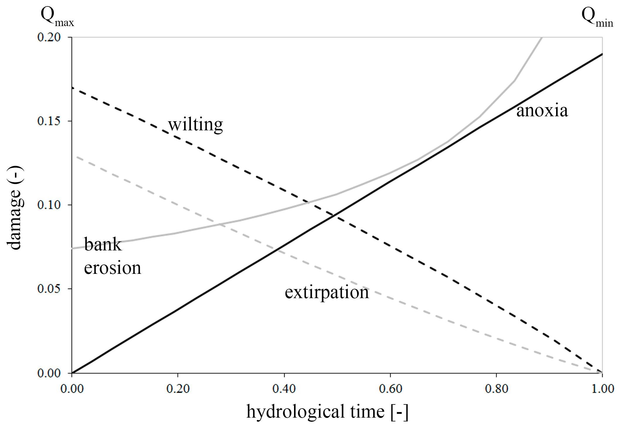
Typically, riverine banks are fully covered by aquatic vegetation, which are completely inundated during the entire hydrological year. In this sense, the minimum discharge mostly influences anoxia, because a large percentage of riparian plants located in the marginal zone are under water (Figure 1). Since anoxia occurs when vegetation is submerged over time, a linear relationship between the damage due to anoxia ΔA(t) and the submergence time, represented by the flow duration curve, can be assumed.
Δ A ( t ) = δ A [ 1 Q ( t ) q Q min q Q max q Q min q ]
At the highest stage, when the discharge is maximum and the submergence time t = 0, the damage ΔA(t) due to anoxia is negligible, and the relative carrying capacity KA(t) tends to one. On the opposite, for the minimum discharge Qmin at the time t = 1, the damage attains a maximum equal to the extremal value ΔA, and the carrying capacity becomes KA(t) = 1 − ΔA. It is worth mentioning that, during the hydrological year, the maximum discharge affects the lowest percentage of riparian vegetation, which is also the farthest from the thalweg; on the contrary, the plants closest to the thalweg are most subjected to submergence, and thus, anoxia.

2.3.2. Wilting

The damage ΔW(t) related to wilting can be assumed to be proportional to the distance of the water level from the water table, which is supposed to have the same elevation of the minimum water level at the time t = 1, and remains constant during the entire hydrological year. As observed above, the closer the vegetation to the thalweg (low discharges), the higher the percentage cover and, therefore, the higher the impact of wilting on the riparian plants at the reach scale.
Following these assumptions and adopting some simplifications [4], the damage associated to wilting can be expressed as:
Δ W ( t ) = δ W [ Q ( t ) 2 3 ( 1 β ) Q min 2 3 ( 1 β ) Q max 2 3 ( 1 β ) Q min 2 3 ( 1 β ) ]
When t = 1 (minimum discharge), the water level coincides with the water table and there is no wilting. Therefore, the damage ΔW(t) is negligible and the carrying capacity KW(t) = 1 − ΔW(t) is equal to one. For t = 0 the flow discharge reaches its maximum and, consequently, the distance from the water table is the largest and the potential damage ΔW(t) attains its maximum value, equal to ΔW.

2.3.3. Extirpation

The damage ΔE(t) related to the extirpation is assumed to be proportional to the energy required to uproot the riparian plants, which is supposed to be proportional to the flow velocity [4].
Δ E ( t ) = δ E [ Q ( t ) 1 β Q min 1 β Q max 1 β Q min 1 β ]
For the minimum discharge, when t = 1, there is no extirpation and the carrying capacity KE(t) reaches a maximum, while for the maximum discharge at t = 0 the damage ΔE(t) attains its maximum value, equal to the extremal value ΔE.

2.3.4. Bank Erosion

The damage ΔB(t) due to bank erosion is assumed to be proportional to the width over depth ratio, which is commonly adopted to describe the braiding tendency, thanks to its role in the transverse river bed evolution [63,64].
Δ B ( t ) = δ B [ Q ( t ) Q min ] 5 β 2 3
where β is the exponent of the width duration curve, frequently adopted to relate flow discharges and transport widths of rivers using a regime equation [4,65].
In this case, for t = 1 (minimum discharge), the damage ΔB(t) reaches its minimum value; while, for higher discharges, the damage increases for braiding river (β > 0.4) and decreases for single-threaded streams (β < 0.4). The extremal value ΔB, therefore, represents the maximum damage during the seasonal cycle for single-threaded rivers and the minimum damage for braiding rivers [4].
Figure 2 shows the trends that the four dimensionless damages considered in the present analysis have in relation to the decrease of the flow discharge, starting from the long-term maximum discharge Qmax and the corresponding dimensionless hydrological time t = 0, towards the time t = 1 that corresponds to the long-term minimum discharge Qmin.

3. Results and Discussion

The sensitivity analysis reported here has been performed by changing the values of initial population P0 and growth rate r of the riparian vegetation, in accordance with available evidence in the established literature [59,60], which is, unfortunately, not exhaustive in addressing these parameters to date. The other parameters, like extremal damages and morphological coefficients, are kept constant and equal to the values obtained by Nones and Di Silvio in their analysis [4], with the aims of reducing the variables used in the present analysis. A further development of the present model, however, would require a site-specific calibration of these parameters too, depending on the river location.
The simulations have been performed assuming a temporal horizon of one hydrological year (i.e., submergence time t spans from 0 to 1), schematized by means of the long-term maximum, minimum, and median discharges and, therefore, the adopted flow duration curve can represent quite well the typical discharge rating curve of the studied rivers. To better describe the influence that the parameters analyzed have with respect to the watercourse sizes, large rivers are also evaluated separately, assuming a total river width Btot > 1000 m as the threshold. Because the main aim of the model is to reproduce the active width of alluvial watercourses, the results report the comparison between measured and computed active river widths, derived from the above reported model. As one can observe, such values are strictly related to the water discharges and the presence of riparian vegetation along the banks. In fact, in adopting the regime equation, one obtains that the lower the discharges, the lower the active width. Similarly, from Equation (4), the vegetational carrying capacity is directly proportional to the water discharge.
In the future, a wider study is yet necessary to assess the relative importance of each parameter and the possibility to rearrange the formulation used, involving other contributions to the total carrying capacity, either increasing the number of species considered or choosing different approaches to describe the population growth, depending on the location of the watercourses under study.

3.1. Initial Population

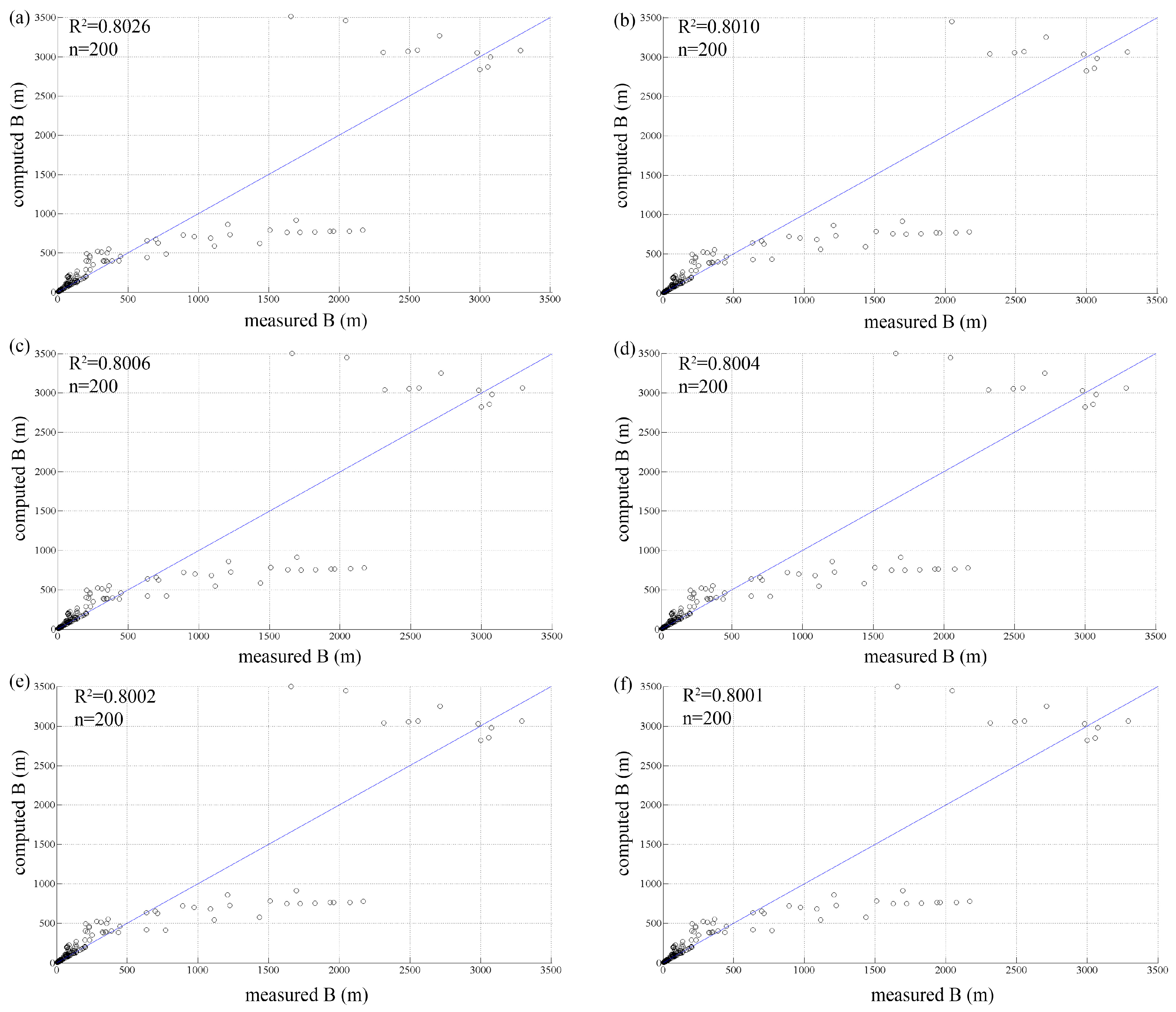
The solution of Equation (4) requires, as an initial condition, an initial population P0 (dimensionless), representing the density of riparian vegetation per unit area at the initial time t = 0. In the literature, very little evidence is available regarding the magnitude of this parameter and the wide range of rivers analyzed here does not permit the selection of a significant value a priori. To overcome these limitations, a sensitivity analysis is performed (Table 1), evaluating the capability of the model in representing the measured active widths B(t) for different values of the initial population P0, which cover some orders of magnitude. The comparison is made in terms of mean relative error E (Equation (12)) and coefficients of determination R2, and the latter is computed for the entire river dataset and only for large rivers.
E = B meas B comp B meas
The other parameters are assumed constant: the extremal damages are the same adopted in [4]: ΔA = 0.19, ΔW = 0.17, ΔE = 0.13, ΔB = 0.31; while the growth rate is imposed equal to 0.025 [59] and the morphological parameters are derived from [65].
In Figure 3 the results of the six tests are shown, highlighting the two groups of rivers analyzed: small Italian watercourses exhibit measured widths of maximum one kilometer, while large rivers can reach values significantly higher. This figure compares the transport (active) widths measured by remote imagery with the ones derived from the vegetation model, starting from the measure of the total width Btot and computing the vegetated width Bv by means of the above reported equations.
As one can observe, the relative error E decreases by increasing the initial population density P0, in particular thanks to the presence of small streams. In fact, regarding the coefficient of determination, on the one hand, for small rivers the model reproduces quite well the active widths, indicating that the impact of the riparian vegetation is relatively small in defining this parameter. On the other hand, in the case of large rivers, the active width is reproduced better for higher values of the initial population P0 (Table 1). Considering all the rivers, for an initial population density greater than 1000 there are no significant changes in the performance of the model against measured widths, indicating a threshold value for this parameter. Intermediate widths (1.5–2.5 km) are not well represented due to the present model structure and possibly because of the data chosen for the calibration: for such reasons, future research is still necessary, considering also the revision of the structure itself and the analyses of more case studies.
Furthermore, for some rivers the present discharge is lower than the bankfull discharge, yielding to inaccuracy in representing active widths by the model. As visible from Figure 3, the computed widths remain quite constant even though the measured ones vary from 1 to 2 km. This inaccuracy can be related to the lower discharges measured during the study and used as inputs for the model. Analyzing the constitutive equations, in fact, it can be noticed that higher flow rates can yield to higher predicted active widths.
The results obtained may lead to the conclusion that the initial population is not a major limiting factor. However, initial values in the range of 100–200 individuals allow for a relatively better evolution of the river in accordance with the model structure, giving rise to computed widths closer to the measured ones, both in the case of small watercourses and for large rivers. As can be observed, the model results are quite insensitive to the initial population and, therefore, additional analyses on a larger database are necessary to confirm these preliminary results, pointing out possible biases related to the parameters adopted. On the other hand, this application could give new insights into the importance of the initial density in simulating the long-term growth of riparian vegetation.

3.2. Vegetation Growth Rate

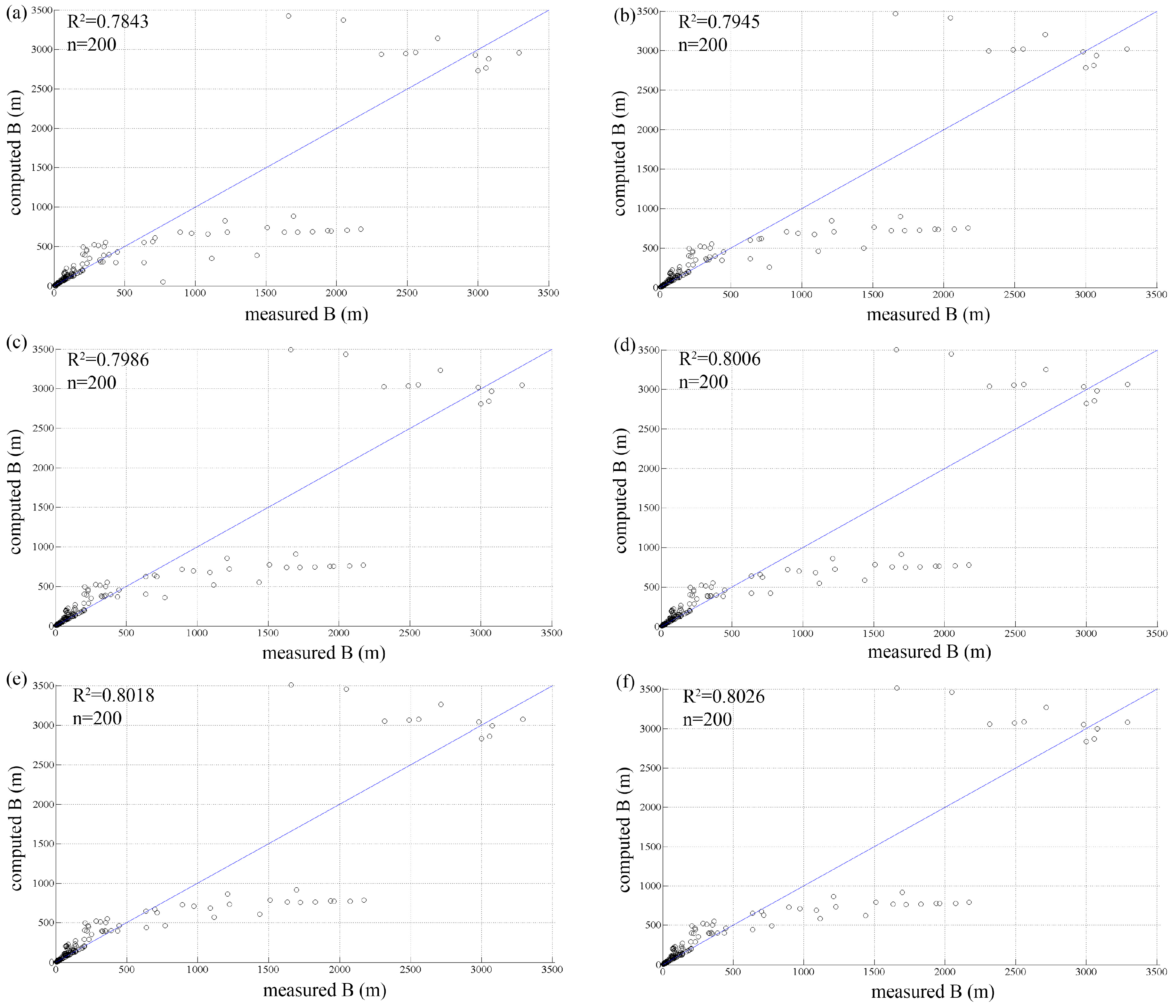
Regardless of the initial density of the plants, the validity of the model is strictly related to the value of the vegetation growth rate r chosen during the simulations, as observable in Figure 4. In the established literature there are specific studies focused on the relative growth rate of various species [58,59,60] and, therefore, for the present study these values are assumed as a basis for the sensitivity analysis. Moreover, values of r outside of the range proposed by the previous studies seem to not have any physical meaning.
In Table 2 the non-dimensional growth rates adopted, the mean relative errors E, and the coefficients of determination R2 for all watercourses and large rivers are reported. In this case, the analysis is performed assuming an initial population P0 = 100, while the other parameters like extremal damages were the ones reported in [4,65] and adopted in the previous analysis. As observed in the previous section, the initial population cannot be considered to be a limiting factor and, consequently, similar results are expected regardless the value of P0 adopted.
In this case, the lower the growth rate, the better the reproduction of the active river width by the model (i.e., the lower the relative errors), especially due to the good representation for large rivers, as highlighted in the following. Similar to the previous analysis, in this case active widths between 1.5 and 2.5 km are also not well represented.
As can be seen from Table 2 and Figure 4, in fact, higher growth rates lead to better representation of the measured river widths, evaluating small and large rivers at the same time. Despite this perception, however, by observing the results it is possible to notice that, for higher growth rates, small Italian rivers are not well represented, while the results for large rivers computed properly. Therefore, intermediate values, like the ones proposed by Gleeson and Tilman [59], allow, in general, for a better assessment of the measured width for the entire database.
From this sensitivity analysis, one can argue that a unique vegetation growth rate is not feasible for reproducing the behavior of two very different fluvial environments (small vs. large rivers) and, hence, the use of calibrated and site-specific vegetation growth rates is suggested for future applications.

4. Conclusions

The present work points out the importance of two biological parameters in defining the active river width by means of a simplified mathematical model. Indeed, the sensitivity analysis of vegetation growth rate and initial density reported here highlights the feedbacks of such parameters in computing the active width, frequently assumed only as dependent of the water discharge (i.e., regime equation). For this first calibration, the model is applied to a relatively small number of cross-sections of small and large rivers, showing the validity of the hypotheses assumed, though highlighting some limitations related to the parameters adopted during the simulations and possible biases in reproducing the measured widths due to many constraints (e.g., river discharges, morphological and biological parameters, etc.). The present model structure is capable of reproducing small and large river widths, but needs improvements to simulate a larger variability of active widths.
As argued in past research [4], the application of the model to other case studies would require some changes of the calibration parameters (extremal damages, vegetal growth rate, initial population, morphological coefficients). Perhaps a revision of the model structure could be required, introducing other contributions to the aggregate carrying capacity, related, for example, to salinity, ice, bottom capillarity, local climate, presence of sediments, groundwater dependency [66], depending on the river location and the local climate.
In spite of the relatively small number of cross-sections studied, the sensitivity analysis showed that the vegetation growth rate plays a major role in defining the vegetated width and, consequently, the active one. For this reason, in evaluating large rivers lower rates are suggested (0.010–0.015), while, for small rivers like the ones studied here, growth rates in the order of 0.03–0.04 can be adopted during the simulations, as suggested by evidence in the existing literature, probably because of the different species involved. The initial population, on the other hand, seems to have a lower influence on the final outcomes of the model. In this case, in fact, the preliminary analysis performed and the related coefficients of determination suggest that a lower initial population is better suitable for small rivers, while a higher initial population can contribute to an improved simulation of the behavior of large rivers. This could be due to the inadequacy of the model in reproducing, at the temporal scale adopted, a fast growth of plants despite the space available.
Notwithstanding the several simplifications adopted in the model and the small database used, the outcomes of this preliminary sensitivity analysis suggest that the basic concepts utilized in the present approach might have a general validity and, therefore, the model could be applied to future case studies aimed at confirming its potential for modelling different environmental conditions. Further research is also necessary: (i) in the estimation of the growth rate, which creates site-specific effects and, therefore, requires a careful evaluation to limit errors in simulating the riparian vegetation growth; (ii) in the definition of the long-term evolution of riparian vegetation, assuming a temporal horizon characterized by a series of consecutive hydrological years; (iii) in the implementation of the model structure, to simulate a larger variability of river widths; (iv) in the integration of this 2D description of the cross-sections with 1D and even 0D models to simulate the very long-term (geological) evolution of rivers.

Author Contributions

Michael Nones developed the mathematical model, while Arianna Varrani performed the simulations. The two authors have contributed equally to writing and editing the paper.

Conflicts of Interest

The authors declare no conflict of interest.

Notation List

The following symbols are used in the manuscript:
Bactive (transport) river width (m)
Bcompcomputed active river width (m)
Bmeasmeasured active river width (m)
Bvvegetated river width (m)
Btottotal river width (m)
Emean relative error (-)
Hwater depth (m)
Kcarrying capacity of the riparian vegetation (-)
Kigeneral carrying capacity (-)
KAcarrying capacity related to anoxia (-)
KWcarrying capacity related to wilting (-)
KEcarrying capacity related to extirpation (-)
KBcarrying capacity related to bank erosion (-)
Koptoptimal carrying capacity (-)
Ppopulation (-)
P0initial population (-)
Qriver discharge (m3·s-1)
Qmaxmaximum river discharge (m3·s-1)
Qminminimum river discharge (m3·s-1)
Qmeanmean river discharge (m3·s-1)
qcoefficient (-)
Rcoefficient of determination (-)
rvegetation growth rate (-)
thydrological time (-)
igeneral damage (-)
Adamage related to anoxia (-)
Wdamage related to wilting (-)
Edamage related to extirpation (-)
Bdamage related to bank erosion (-)
αcoefficient of the width duration curve (-)
βexponent of the width duration curve (-)
ΔAextremal damage related to anoxia (-)
ΔWextremal damage related to wilting (-)
ΔEextremal damage related to an extirpation (-)
ΔBextremal damage related to bank erosion (-)
γvariability coefficient of river discharge (-)

References

  1. Marchetti, M. Environmental changes in the central Po Plain (Northern Italy) due to fluvial modifications and anthropogenic activities. Geomorphology 2002, 44, 361–373. [Google Scholar] [CrossRef]
  2. Naiman, R.J.; Dècamps, H. The ecology of interfaces: Riparian zones. Annu. Rev. Ecol. Syst. 1997, 28, 621–658. [Google Scholar] [CrossRef]
  3. Kramer, K.; Vreugdenhil, S.J.; van der Werf, D.C. Effects of flooding on the recruitment, damage and mortality of riparian tree species: A field and simulation study on the Rhine floodplain. For. Ecol. Manag. 2008, 255, 3893–3903. [Google Scholar] [CrossRef]
  4. Nones, M.; Di Silvio, G. Modeling of river width variations based on hydrological, morphological and biological dynamics. J. Hydraul. Eng. 2016, 142. [Google Scholar] [CrossRef]
  5. Wilson, C.A.M.E.; Yagci, O.; Rauch, H.-P.; Olsen, N.R.B. 3D Numerical modelling of a willow vegetated river/floodplain system. J. Hydrol. 2006, 327, 13–21. [Google Scholar] [CrossRef]
  6. Li, C.W.; Zeng, C. 3D Numerical modelling of flow divisions at open channel junctions with or without vegetation. Adv. Water Resour. 2009, 32, 49–60. [Google Scholar] [CrossRef]
  7. Bockelmann, B.N.; Fenrich, E.K.; Lin, B.; Falconer, R.A. Development of an ecohydraulics model for stream and river restoration. Ecol. Eng. 2004, 22, 227–235. [Google Scholar] [CrossRef]
  8. Abu-Aly, T.R.; Pasternack, G.B.; Wyrick, J.R.; Barker, R.; Massa, D.; Johnson, T. Effects of LiDAR-derived, spatially distributed vegetation roughness on two-dimensional hydraulics in a gravel-cobble river at flows of 0.2 to 20 times bankfull. Geomorphology 2014, 206, 468–482. [Google Scholar] [CrossRef]
  9. Nones, M.; Guerrero, M.; Ronco, P. Opportunities from low-resolution modelling of river morphology in remote parts of the world. Earth Surf. Dyn. 2014, 2, 9–19. [Google Scholar] [CrossRef] [Green Version]
  10. Micheli, E.R.; Kirchner, J.W. Effects of wet meadow riparian vegetation on streambank erosion. 1. Remote sensing measurements of streambank migration and erodibility. Earth Surf. Process. Landf. 2002, 27, 627–639. [Google Scholar] [CrossRef]
  11. Mitsch, W.J.; Gosselink, J. Wetlands; Wiley & Sons: New York, NY, USA, 2007. [Google Scholar]
  12. Lange, C.; Schneider, M.; Mutz, M.; Haustein, M.; Halle, M.; Seidel, M.; Sieker, H.; Wolter, C.; Hinkelmann, R. Model-based design for restoration of a small urban river. J. Hydro-Environ. Res. 2015, 9, 226–236. [Google Scholar] [CrossRef]
  13. Manner, R.B.; Wilcox, A.C.; Kui, L.; Lightbody, A.F.; Stella, J.C.; Sklar, L.S. When do plants modify fluvial processes? Plant-hydraulic interactions under variable flow and sediment supply rates. J. Geophys. Res. 2015, 120, 325–345. [Google Scholar] [CrossRef]
  14. Camporeale, C.; Perucca, E.; Ridolfi, L.; Gurnell, A.M. Modeling the interactions between river morphodynamics and riparian vegetation. Rev. Geophys. 2013, 51, 379–414. [Google Scholar] [CrossRef]
  15. Osterkamp, W.R.; Hupp, C.R. Geomorphic and vegetative characteristics along three northern Virginia streams. Geol. Soc. Am. Bull. 1984, 95, 1093–1101. [Google Scholar] [CrossRef]
  16. Hupp, C.R.; Osterkamp, W.R. Bottomland vegetation distribution along Passage Creek, Virginia, in relation to fluvial landforms. Ecology 1985, 66, 670–681. [Google Scholar] [CrossRef]
  17. Mahoney, J.M.; Rood, S.B. Streamflow requirements for cottonwood seedling recruitment: An integrative model. Wetlands 1998, 18, 634–645. [Google Scholar] [CrossRef]
  18. Bendix, J.; Hupp, C.R. Hydrological and geomorphological impacts on riparian plant communities. Hydrol. Process. 2000, 14, 2977–2990. [Google Scholar] [CrossRef]
  19. Auble, G.T.; Friedman, J.M.; Scott, M.L. Relating riparian vegetation to present and future streamflows. Ecolog. Appl. 1994, 3, 544–554. [Google Scholar] [CrossRef]
  20. Friedman, J.M.; Auble, G.T. Mortality of riparian box elder from sediment mobilization and extended inundation. Regul. Rivers Res. Manag. 1999, 15, 463–476. [Google Scholar] [CrossRef]
  21. Johnson, W.C. Tree recruitment and survival in rivers: Influence of hydrological processes. Hydrol. Process. 2000, 14, 3051–3074. [Google Scholar] [CrossRef]
  22. Lite, S.J.; Bagstad, K.J.; Stromberg, J.C. Riparian plant species richness along lateral and longitudinal gradients of water stress and flood disturbance, San Pedro River, Arizona, USA. J. Arid Environ. 2005, 63, 785–813. [Google Scholar] [CrossRef]
  23. Tealdi, S. River-Riparian Vegetation Interactions. Ph.D. Thesis, Politecnico of Torino, Turin, Italy, May 2012. [Google Scholar]
  24. Tewari, S.; Kulhavy, J.; Rock, B.N.; Hadas, P. Remote monitoring of forest response to changed soil moisture regime due to river regulation. J. For. Sci. 2003, 49, 429–438. [Google Scholar]
  25. Yanosky, T.M. Effects of Flooding upon Woody Vegetation along Parts of the Potamac River Floodplain; U.S. Geological Survey Professional Paper; U.S. Geological Survey: Reston, VA, USA, 1982.
  26. Osterkamp, W.R.; Costa, J.E. Change accompanying an extraordinary flood on sandbed stream. In Catastrophic Flooding; Allen and Unwin: St. Leonards, Australia, 1987. [Google Scholar]
  27. Kozlowski, T.T. Responses of woody plants to flooding. In Tree Physiology Monograph; Heron Publishing: Victoria, BC, Canada, 1984. [Google Scholar]
  28. Naumburg, E.; Mata-Gonzales, R.; Hunter, R.G.; McLendon, T.; Martin, D.W. Phreatophytic vegetation and groundwater fluctuations: A review of current research and application of ecosystem response modelling with an emphasis on great basin vegetation. Environ. Manag. 2005, 35, 726–740. [Google Scholar] [CrossRef] [PubMed]
  29. Hupp, C.R. Plant ecological aspects of flood geomorphology and paleoflood history. In Flood Geomorphology; Wiley & Sons: New York, NY, USA, 1988. [Google Scholar]
  30. McKenney, R.; Jacobson, R.B.; Wertheimer, R.C. Woody vegetation and channel morphogenesis in low-gradient, gravel-bed streams in the Ozrak Plateaus, Missouri and Arkansas. Geomorphology 1995, 13, 175–198. [Google Scholar] [CrossRef]
  31. Richter, B.D.; Richter, H.E. Prescribing flood regimes to sustain riparian ecosystem along meandering rivers. Conserv. Biol. 2000, 14, 1467–1478. [Google Scholar] [CrossRef]
  32. Gurnell, A.M.; Petts, E.; Hannah, D.M.; Smith, B.P.G.; Edwards, P.J.; Kollmann, J.; Ward, J.V.; Tockner, K. Riparian vegetation and island formation along the gravel-bed Fiume Tagliamento, Italy. Earth Surf. Process. Landf. 2001, 26, 31–62. [Google Scholar] [CrossRef]
  33. Franz, E.H.; Bazzaz, F.A. Simulation of vegetation response to modified hydrological regimes: A probabilistic model based on niche differentiation in a floodplain forest. Ecology 1977, 58, 176–183. [Google Scholar] [CrossRef]
  34. Stromberg, J.C.; Patten, D.T. Instream flow requirements for cottonwoods at Bishop Creek, Inyo County, California. Rivers 1991, 2, 1–11. [Google Scholar]
  35. Pearlstine, L.; McKellar, H.; Kitchens, W. Modelling the impacts of a river diversion on bottomland forest communities in the Santee River Floodplain, South Carolina. Ecol. Model. 1985, 29, 283–302. [Google Scholar] [CrossRef]
  36. Brookes, C.J.; Hooke, M.J.; Mant, J. Modelling vegetation interactions with channel flow in river valleys of the Mediterranean region. Catena 2000, 40, 93–118. [Google Scholar] [CrossRef]
  37. Lytle, D.A.; Merritt, D.M. Hydrologic regimes and riparian forests: A structured population model for cottonwood. Ecology 2004, 85, 2493–2503. [Google Scholar] [CrossRef]
  38. Gran, K.; Paola, C. Riparian vegetation controls on braided stream dynamics. Water Resour. Res. 2001, 37, 3275–3283. [Google Scholar] [CrossRef]
  39. Camporeale, C.; Ridolfi, L. Riparian vegetation distribution induced by river flow variability: A stochastic approach. Water Resour. Res. 2006, 42, W10415. [Google Scholar] [CrossRef]
  40. Muneepeerakul, R.; Rinaldo, A.; Rodriguez-Iturbe, I. Effects of river flow scaling properties on riparian width and vegetation biomass. Water Resour. Res. 2007, 43. [Google Scholar] [CrossRef]
  41. Camporeale, C.; Ridolfi, L. Interplay among river meandering, discharge stochasticity and riparian vegetation. J. Hydrol. 2010, 382, 138–144. [Google Scholar] [CrossRef]
  42. Tealdi, S.; Camporeale, C.; Ridolfi, L. Modeling the impact of river damming on riparian vegetation. J. Hydrol. 2011, 396, 302–312. [Google Scholar] [CrossRef]
  43. Conway, D. The climate and hydrology of the Upper Blue Nile River. Geogr. J. 2000, 166, 49–62. [Google Scholar] [CrossRef] [Green Version]
  44. Pasanisi, F.; Tebano, C.; Zarlenga, F. A Survey near Tambara along the Lower Zambezi River. Environments 2016, 3, 6. [Google Scholar] [CrossRef]
  45. Ministero LL. PP. Servizio Idrografico. In Annali Idrologici Italia; Ministero LL. PP.: Roma, Italy, 1951. (In Italian) [Google Scholar]
  46. Di Silvio, G.; Nones, M. Morphodynamic reaction of a schematic river to sediment input changes: Analytical approaches. Geomorphology 2014, 215, 74–82. [Google Scholar] [CrossRef]
  47. Duarte, P.; Meneses, R.; Hawkins, A.J.S.; Zhu, M.; Fang, J.; Grant, J. Mathematical modelling to assess the carrying capacity for multi-species culture within coastal waters. Ecol. Model. 2003, 168, 109–143. [Google Scholar] [CrossRef]
  48. Bhowmik, N.G.; Stall, J.B. Hydraulic Geometry and Carrying Capacity of Floodplains; Research Report; University of Illinois: Champaign, IL, USA, 1979. [Google Scholar]
  49. Yalin, M.S. River Mechanics; Pergamon Press: Oxford, UK, 1992. [Google Scholar]
  50. Singh, V.P. On the theories of hydraulic geometry. Int. J. Sediment Res. 2003, 18, 196–218. [Google Scholar]
  51. Parker, G.; Wilcock, P.R.; Paola, C.; Dietrich, W.E.; Pitlick, J. Physical basis for quasi-universal relations describing bankfull hydraulic geometry of single-thread gravel bed rivers. J. Geophys. Res. 2007, 112. [Google Scholar] [CrossRef]
  52. Vianello, A.; D’Agostino, V. Bankfull width and morphological units in an alpine stream of the dolomites (Northern Italy). Geomorphology 2007, 83, 266–281. [Google Scholar] [CrossRef]
  53. Valiani, A.; Caleffi, V. Analytical findings for power law cross-sections: Uniform flow depth. Adv. Water Resour. 2009, 32, 1404–1412. [Google Scholar] [CrossRef]
  54. Wilkerson, G.W.; Parker, G. Physical basis for quasi-universal relations describing bankfull hydraulic geometry of sand-bed rivers. J. Hydraul. Eng. 2010, 137, 739–753. [Google Scholar] [CrossRef]
  55. Nones, M.; Ronco, P.; Di Silvio, G. Modelling the impact of large impoundments on the lower Zambezi River. Int. J. River Basin Manag. 2013, 11, 221–236. [Google Scholar] [CrossRef]
  56. Verhulst, P.-F. Notice sur la loi que la population poursuit dans son accroissement. Corresp. Math. ET Phys. 1838, 10, 113–121. [Google Scholar]
  57. Gabriel, J.-P.; Saucy, F.; Bersier, L.-F. Paradoxes in the logistic equation? Ecol. Model. 2005, 185, 147–151. [Google Scholar] [CrossRef]
  58. Grime, J.P.; Hunt, T. Relative growth-rate: Its range and adaptive significance in a local Flora. J. Ecol. 1975, 63, 393–422. [Google Scholar] [CrossRef]
  59. Gleeson, S.K.; Tilman, D. Plant Allocation, Growth Rate and Successional Status. Funct. Ecol. 1994, 8, 543–550. [Google Scholar] [CrossRef]
  60. Hunt, R.; Cornelissen, J.H.C. Components of relative growth rate and their interrelations in 59 temperate plant species. New Phytol. 1997, 135, 395–417. [Google Scholar] [CrossRef]
  61. Karrenberg, S.; Edwards, P.J.; Kollmann, J. The life history of Salicaceae living in the active zone of floodplains. Freshw. Biol. 2002, 47, 733–748. [Google Scholar] [CrossRef]
  62. Merritt, D.M.; Scott, M.L.; Poff, N.L.; Auble, G.T.; Lytle, D.A. Theory, methods and tools for determining environmental flows for riparian vegetation: Riparian vegetation-flow response guilds. Freshw. Biol. 2010, 55, 206–225. [Google Scholar] [CrossRef]
  63. Rosgen, D.L. A classification of natural rivers. Catena 1994, 22, 169–199. [Google Scholar] [CrossRef]
  64. Schumm, S.A. Patterns of alluvial rivers. Annu. Rev. Earth Planet. Sci. 1985, 13, 5–27. [Google Scholar] [CrossRef]
  65. Nones, M. Riverine Dynamics at Watershed Scale: Hydro-Morpho-Biodynamics in Rivers; Lambert Academic Publishing: Saarbrücken, Germany, 2013; p. 140. [Google Scholar]
  66. Hoyos, I.C.P.; Krakauer, N.Y.; Khanbilvardi, R. Estimating the probability of vegetation to be groundwater dependent based on the evaluation of tree models. Environments 2016, 3, 9. [Google Scholar] [CrossRef]
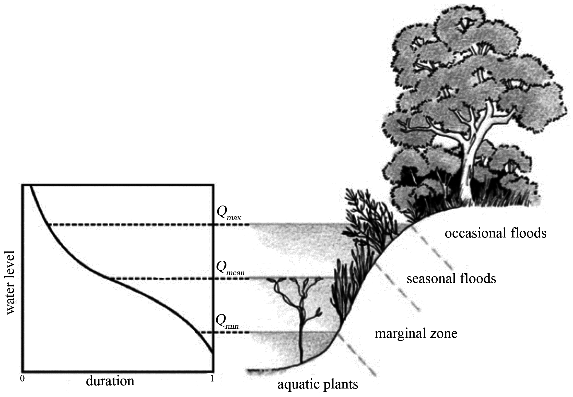
Figure 1. Scheme of alluvial river: riparian vegetation and water flow.
Environments 03 00030 g001
Figure 2. Example of damage variations related to the hydrological time, starting from the maximum discharge Qmax at t = 0 to the minimum discharge Qmin at t = 1.
Environments 03 00030 g002
Figure 3. Comparison between computed and measured active river width B for different initial populations (P0): (a) P0 = 10; (b) P0 = 50; (c) P0 = 100; (d) P0 = 200; (e) P0 = 500; (f) P0 = 1000.
Environments 03 00030 g003
Figure 4. Comparison between computed and measured active river width B for different growth rates (r): (a) r = 0.010; (b) r = 0.015; (c) r = 0.020; (d) r = 0.025; (e) r = 0.030; (f) r = 0.035.
Environments 03 00030 g004
Table 1. Sensitivity analysis of the initial population P0.
TestP0ER2R2 Large Rivers
test 1100.34520.80260.7347
test 2500.34050.80100.7459
test 31000.33940.80060.7488
test 42000.33880.80040.7505
test 55000.33820.80020.7517
test 610000.33820.80010.7521
P0: Initial population; E: Relative error; R2: Coefficient of determination.
Table 2. Sensitivity analysis of the vegetation growth rate r.
TestrER2R2 Large Rivers
test 10.0100.31570.78430.8544
test 20.0150.32230.79450.7898
test 30.0200.33230.79860.7630
test 40.0250.33940.80060.7488
test 50.0300.34400.80180.7401
test 60.0350.34740.80260.7344