A Two-Stage Machine Learning Framework for Air Quality Prediction in Hamilton, New Zealand

Abstract

Air quality significantly affects human health, productivity, and overall well-being. This study applies machine learning techniques to analyse and predict air quality in Hamilton, New Zealand, focusing on particulate matter (PM2.5 and PM10) and environmental factors such as temperature, humidity, wind speed, and wind direction. Data were collected from two monitoring sites (Claudelands and Rotokauri) to explore relationships between variables and evaluate the performance of different predictive models. First, the unsupervised k-means clustering algorithm was used to categorise air quality levels based on data from one or both locations. These cluster labels were then used as target variables in supervised learning models, including random forests, decision trees, support vector machines, and k-nearest neighbours. Model performance was assessed by comparing prediction accuracy for air quality at either Claudelands or Rotokauri. Results show that the random forest (93.6%) and decision tree (91.8%) models outperformed k-nearest neighbours (KNN, 83%) and support vector machine (SVM, 61%) in predicting air quality clusters derived from k-means analysis. The three clusters (very good, good, and moderate) reflected seasonal and urban–semi-urban gradients, while cross-location validation confirmed that models trained at Claudelands generalised effectively to Rotokauri, demonstrating scalability for regional air quality forecasting. These findings highlight the potential of combining clustering with supervised learning to improve air quality predictions. Such methods could support environmental monitoring and inform strategies for mitigating pollution-related health risks in New Zealand cities and beyond.

1. Introduction

The air quality index (AQI) is monitored by regional and district councils for planning purposes, particularly in areas experiencing significant industrial growth and land-use intensification [1,2]. The AQI is reported with the following classification (good, moderate, unhealthy, and hazardous) annually by Land Air Water Aotearoa (LAWA) in New Zealand and is used to inform policies and procedures necessary to maintain or improve the air quality as it impacts the population’s health [3]. Outdoor air quality not only impacts the health of those spending time outdoors, but also has a big impact on indoor air quality (IAQ) as it is drawn in by ventilation and air-conditioning systems, and hence significantly impacts the health of those spending time indoors. Fanger [4] illustrated how this negative impact could be found with poor IAQ, impacting respiratory health, and exacerbating allergies and asthma. Boamponsem et al. [5] analysed the sources and trends of outdoor pollutants in Auckland, New Zealand between 2006 and 2016, attributed them to traffic emissions and biomass burning, and identified a pressing need to enhance air quality to protect public health. Ancelet et al. [6] performed a similar study on PM10 in Nelson, New Zealand and found distinct diurnal patterns with morning and evening peaks primarily driven by biomass combustion, with additional contributions from vehicles, marine aerosols, shipping sulfates, and crustal matter. This indicates that both anthropogenic sources, such as residential heating and traffic, and natural phenomena, such as sea spray aerosols, significantly influence local air quality. While the Auckland and Nelson air quality studies focus on understanding pollution sources and trends to inform targeted emission reduction strategies, [7], in their analysis of Toronto’s transit system, highlight the importance of climate change on outdoor air quality and adapting urban transit management practices to evolving environmental conditions. Both contexts highlight the necessity of integrating climate and environmental considerations into urban planning to mitigate adverse effects on public health, infrastructure reliability, and overall urban resilience [7].

In Hamilton, New Zealand, Williams et al. [8] compared the particulate matter (PM2.5) between classrooms based in the central city campus and others based on the rural fringe of Hamilton as a semi-urban. The results also indicate that when outdoor PM2.5 levels exceed the city council threshold of 25 μg/m³, the impact is proportionally reflected in the indoor readings. This effect varies between urban and semi-urban areas and is more pronounced in semi-urban settings.

1.1. Machine Learning in Air Quality

Muthukumar et al. [9] note that to estimate the patterns and correlations for PM2.5, we need to understand the behaviour of these air pollution indicators to predict it in advance. Therefore, this prediction requires advanced deep learning predictive models to achieve a new air quality index customised for each city and region. Therefore, researchers conducted spatiotemporal air quality analysis to achieve a correlation with the seasonal changes in PM2.5 levels using different machine learning tools [10,11]. Machine learning using satellite data enhances air quality modelling by addressing challenges such as spatial variability, imbalanced data, and effective model validation and interpretation, and data could be sent to a foresight lab to conduct further predictive analysis and compare urban and industrial air quality data. This approach improves the accuracy and generalisability of models, benefiting environmental management and health assessments for air pollutants and greenhouse gases [12]. Ravindiran et al. [13] examined the air quality index for the Indian state of Andhra Pradesh’s Visakhapatnam city using machine learning models such as the light gradient boosting machine (LightGBM), random forest, Gatboost, AdaBoost, and XGboost to forecast the AQI. Their machine learning models predicted the AQI, with the random forest and Gatboost models showing maximum correlations of 0.9998 and 0.9936, respectively. Gupta et al. [14] used three different algorithms to draw a comparative analysis of the AQI values of several cities in India using different parameters, such as PM2.5 and PM10, due to high population density. These algorithms were the support vector regression (SVR), random forest regression (RFR), and CatBoost regression (CR). The RFR and CR models provided high accuracy compared to the synthetic minority oversampling technique (SMOTE) algorithm. Additionally, their results indicate that some algorithms proved to be more accurate for cities than others. For example, CR gave the highest accuracy for New Delhi and Bangalore cities; however, RFR came with the highest accuracy in Kolkata and Hyderabad.

Senthivel and Chidambaranathan [15] explored different machine learning tools to forecast and classify the AQI for a selected city. These tools could generate different accuracies; therefore, it is important to profile the right tool for each city. They used logistic regression, gradient boosting (GB), decision tree (DT), deep natural networks (DNN), support vector regression, a support vector classifier, random forest tree, naive Bayes classifier, and k-nearest neighbour. The results show that the algorithms for naive Bayes, GB regression, and deep natural networks are recommended for forecasting AQI. However, the results show that logistic regression is recommended for predicting classes. Additionally, the results conclude that each dataset and geographical area would require different machine learning techniques.

Zhang et al. [16] presented a comprehensive survey for AQ prediction using deep learning with a focus on research conducted for the period of 2017–2023 in different study areas such as China, the USA, India, Iran, Spain, Korea, and Saudi Arabia. These studies stressed the importance of selecting a suitable algorithm for each city based on the population size and industrial activities. The mean absolute percentage error (MAPE) was 0.698 using spatial attention-embedded (SpAttRNN) [17] and 8.07 using a combined empirical mode decomposition (EMD) of LSTM with improved particle swarm optimisation (IPSO) to become EMD-IPSO-LSTM [18] in Beijing.

Zaini et al. [19] found that the ensemble empirical mode decomposition and long short-term memory (EEMD-LSTM) hybrid model is the recommended method for forecasting PM2.5 as this model outperformed other deep learning models for AQI prediction for urban areas, such as Kuala Lumpur, West Malaysia, with high industrial activities and urbanisation. The proposed method decreased the forecasting error compared to the empirical mode decomposition with long short-term memory architecture by 49.49% regarding root mean square error (RMSE).

Zhao et al. [20] found that the hybrid deep learning framework outperformed traditional models for AQI prediction during the COVID-19 pandemic in Wuhan and Shanghai. They found that lockdowns improved AQI prediction accuracy using the long-term short-term memory network (LSTM) and the bidirectional LSTM (Bi-LSTM).

Li and Jiang [21] demonstrated that advanced hybrid models such as the Loess STL-TCN-BiLSTM with dependency matrix attention can predict multiple air pollutants (including PM2.5 and PM10) with high accuracy in Beijing, achieving mean absolute percentage errors as low as 6.8%. Similarly, Mohammadi et al. [22] evaluated nine years of PM2.5 data from Isfahan, Iran, across several machine learning algorithms and found that artificial neural networks (ANNs) achieved the best performance (91.1% accuracy), outperforming KNN, SVM, and random forest. Vieru and Cărbureanu [23], using data from 30 Romanian cities, highlighted AdaBoost and gradient boosting as being the most effective for real-time air quality prediction. In Russian cities, Gladkova and Saychenko [24] showed that LSTM outperformed ARIMA and Facebook Prophet for three-month PM2.5 forecasts, achieving the lowest RMSE. Bai et al. [25] further emphasised the value of hybrid deep learning approaches, where a CNN-LSTM model reached 91% accuracy in predicting PM2.5 in Qingdao, China. Collectively, these studies confirm that ensemble and deep learning approaches can capture the complex, nonlinear relationships between pollutants and meteorological factors, supporting our two-stage framework that combines clustering with supervised learning for localised air quality prediction in Hamilton.

Bellinger et al. [26] surveyed 400 articles and identified 47 of these articles illustrating the processes using data mining in air pollution epidemiology with the aim to forecast these data based on recorded life data from 2000 to 2017. These studies identify three primary research areas: source apportionment, forecasting, and hypotheses for the increased use of machine learning applications. In England, Wood [27] analysed trend attributes for PM2.5 forecasting using data from 2018 to 2022, while in Türkiye, Gundogdu and Elbir [28] conducted a similar analysis using data from 2020 to 2021. Both studies relied on publicly available data from densely populated cities. The Wood [27] study shows the mean PM2.5 average hourly values around 5.74–11.27 µg/m³. However, the Türkiye PM2.5 ranges from 0.1 to 209.7 µg/m³ with a standard deviation of 16.1 and 11.8 µg/m³, respectively [28]. The results show that the nonlinear autoregressive with exogenous inputs (NARX) model achieved a high score of 89% for Türkiye. However, the supervised machine learning models (SML) method used for England cities by Wood [27] achieved a mean averaged error (MAE) range of 1–3 µg/m³ for t0 to t + 3 h ahead. Huang et al. [18] used three representative meteorological monitoring stations in Beijing, China, for the following period: 1 January 2020 to 31 December 2020. This study suggested combining empirical mode decomposition (EMD) with a gated recurrent unit (GRU) to predict PM2.5 concentrations, achieving improved results compared to single models with the support of using the LSTM algorithm.

1.2. Urban Pollution Forecasting

In New Zealand, the air quality is checked and reported by local councils and organisations, such as Land Air Water Aotearoa (LAWA), who help guide decisions for the environment and public safety [3]. These reports usually put air quality into categories such as good, moderate, unhealthy, or hazardous, and they are helpful for councils to decide how to respond, especially in cities where there is more traffic or growing industry [1,2]. Outdoor air quality not only affects individuals who spend significant time outside, but also plays a crucial role in determining indoor air quality (IAQ), as pollutants are drawn indoors via ventilation systems [4]. Poor IAQ has been linked to a range of adverse health effects, including respiratory illnesses, allergies, and asthma [4]. Studies across various cities in New Zealand highlighted the influence of anthropogenic activities on outdoor air pollution. For example, Boamponsem et al. [5] identified vehicular emissions and biomass combustion as dominant contributors to PM2.5 levels in Auckland between 2006 and 2016, while Ancelet et al. [6] observed diurnal PM10 peaks in Nelson attributed primarily to residential wood burning and shipping activity.

Despite increasing interest in machine learning (ML) for air quality forecasting globally [10,13,16], New Zealand-specific studies remain limited in scope and application. Internationally, researchers employed a wide range of models, including decision trees, support vector machines, and deep learning architectures, such as LSTM and CNN-LSTM, to model air quality patterns in large metropolitan regions, such as Beijing, Kuala Lumpur, and Visakhapatnam [17,19,25]. These models demonstrated success in capturing nonlinear pollutant behaviour, enhancing spatial resolution, and improving short-term forecasts [18,20,21]. However, such techniques have been largely underutilised in medium-sized New Zealand cities, where datasets are more fragmented and environmental conditions vary significantly between locations.

1.3. Aim of This Study

Current air quality studies in Hamilton are mostly descriptive or observational, focusing on single-point measurements or trend analysis without predictive modelling [8]. There is a lack of research applying integrated ML approaches combining unsupervised (clustering) and supervised (classification) methods to generate AQI categories and forecast pollution levels across multiple urban and semi-urban sites. Moreover, no existing study tested model application by training on one location (e.g., Claudelands) and predicting on another (e.g., Rotokauri), which is essential for validating real-world applicability. This absence of cross-location validation and clustering-informed prediction limits the ability of environmental agencies to deploy scalable, adaptive models for public use.

This study addresses the above gaps by leveraging machine learning to classify and predict air quality trends at two spatially distinct sites in Hamilton Claudelands (urban) and Rotokauri (semi-urban). Using a two-stage approach, we first apply k-means clustering to derive natural groupings in air quality data, followed by the use of supervised models, including decision trees, random forests, support vector machines, and k-nearest neighbours, to predict AQI clusters. Data pre-processing steps, such as rolling averages, imputation, and feature harmonisation, are used to ensure temporal and spatial consistency.

The aim of this study is twofold: (1) to assess the performance of widely used machine learning models on short-term urban air quality prediction, and (2) to examine whether combining clustering with supervised methods improves predictive performance relative to standalone approaches. While not intended as a fully developed technological innovation at this stage, the study contributes methodological innovation by demonstrating that cluster-informed modelling enhances both interpretability and predictive accuracy. In this way, the study provides practical insights for medium-sized cities with limited monitoring infrastructure while advancing methodological approaches for air quality prediction.

This work not only contributes to the emerging field of AI-driven environmental monitoring in Aotearoa, New Zealand, but also aligns with sustainable development goals (SDG 3: Good Health and Well-being; SDG 11: Sustainable Cities and Communities) by promoting proactive air quality management; that is, enabling early prediction of pollution episodes and supporting timely interventions by councils and communities rather than relying solely on reactive responses.

• Each city requires a special algorithm to predict the AQI to forecast the particulate matters such as PM2.5 and PM10. This is necessary to meet the sustainable development goals (SDGs) for health and improving urban sustainability, aligning with SDG 3 (Good Health and Well-being) and SDG 11 (Sustainable Cities and Communities).
• Prediction of outdoor AQI trends based on data from prior years can assist in assessing the risk of increased particulate matter when extrapolating or transferring data from one sensor location to another, thereby enabling a more reliable interpretation of spatial air quality patterns rather than directly mitigating the risk itself.
• We predict and forecast the PM2.5 at a specific location, such as semi-urban, and compare it with two air quality monitoring systems based in the Hamilton city centre. The locations for the stations are Hamilton Airshed-Claudelands and Hamilton Airshed-Bloodbank, at a distance from our specific location of 5.7 km and 6.78 km, respectively.

2. Materials and Methods

2.1. Overview

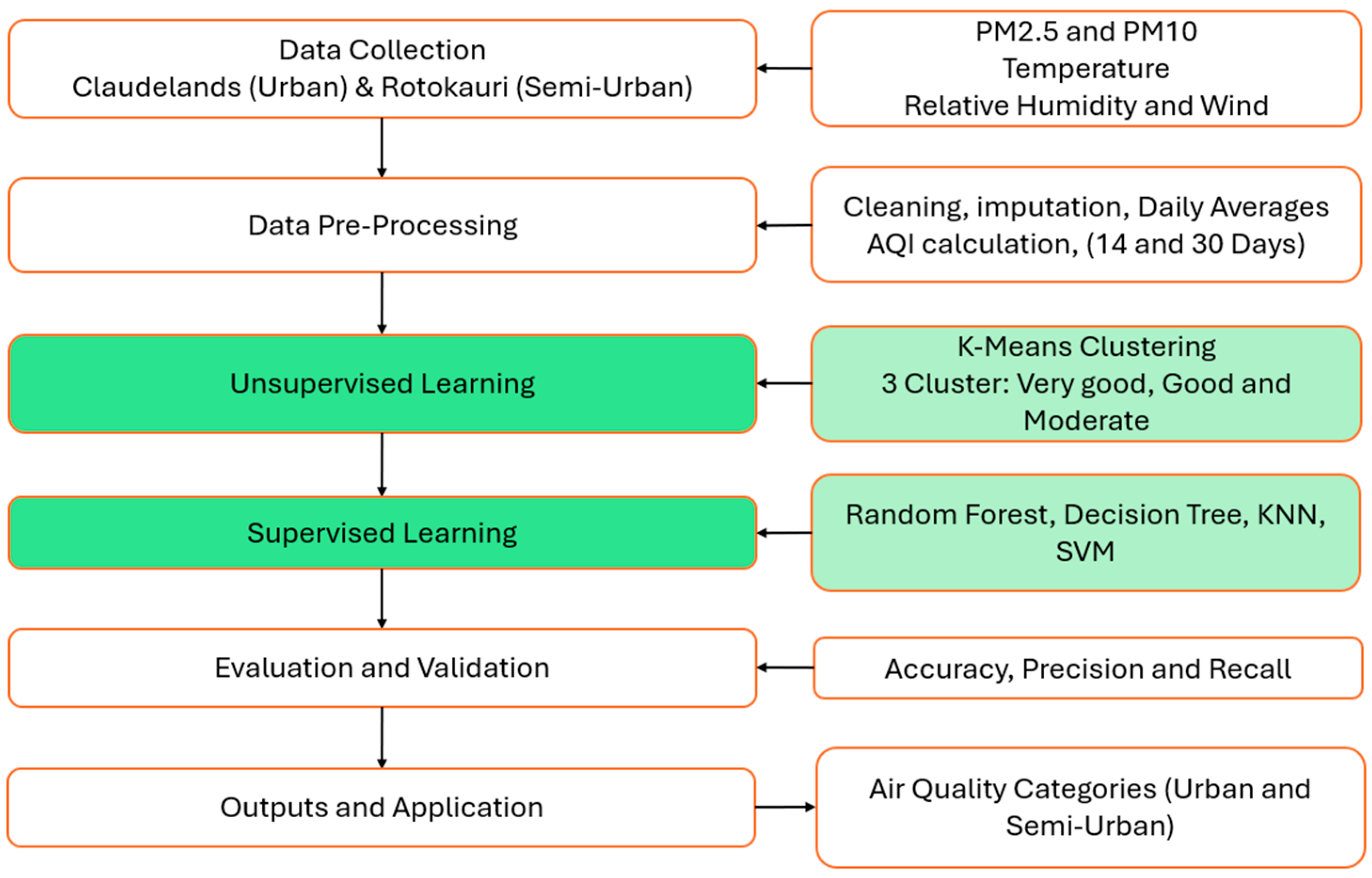
An overview of the methodology is illustrated in Figure 1. It begins with data collection from two monitoring sites in Hamilton: Claudelands (urban) and Rotokauri (semi urban), as shown in Figure 1. The datasets included pollutant concentrations (PM2.5 and PM10) alongside key meteorological variables such as temperature, humidity, wind speed, and wind direction. The next stage involved data pre-processing to ensure consistency and quality. This included cleaning and formatting the datasets through time alignment, unit harmonisation, and imputation of missing values. The data were then down-sampled to daily averages to minimise outlier effects, and the air quality index (AQI) was calculated. Rolling statistical windows (14 day and 30 day) were applied to smooth temporal variations and highlight both short term fluctuations and long-term seasonal trends. In the unsupervised learning stage, k-means clustering was employed to categorise the data into three groups representing air quality levels: very good, good, and moderate. These clusters reflected both seasonal variation and the contrasts between urban and semi urban environments. The supervised learning stage used these cluster labels as targets to train four machine learning classifiers: random forest, decision tree, k-nearest neighbours (KNN), and support vector machine (SVM). Common features across sites (PM2.5, PM10, temperature, and AQI) were selected as predictors, with models trained on Claudelands data and evaluated on Rotokauri data (approximately an 80:20 ratio by record counts).

The study area covers two urban locations in Hamilton city, New Zealand. One of the locations, Claudelands, hosts the “Hamilton Airshed” air quality station maintained by the Waikato Regional Council [29]. The other monitored location is at Wintec Rotokauri Campus, where a research data collection site has been established recently [30]. A map of Hamilton city from OpenStreetMap contributors [31] visualises the two air quality monitoring locations in Figure 2. A major highway (State Highway 1C) runs between the two air quality stations. Some farms and industrial factories are also located near the Rotokauri station. The Claudelands station is situated near residential and shopping areas. The Rotokauri station surroundings are less densely populated than the Claudelands station area.

Hamilton is the fourth largest city in New Zealand and a key economic hub in the Waikato region [32]. It has an area of approximately 110 km² and a population of approximately 174,741 [33]. This gives it a population density of approximately 1600/km². The city plays a significant role in New Zealand’s economy, particularly in agriculture, education, and research, contributing to the national GDP through its thriving dairy industry and the presence of the University of Waikato [33]. However, air pollution remains a growing concern due to vehicle emissions, residential wood burning, and industrial activities, which can impact urban air quality and public health [34]. Therefore, this study selected Hamilton as the area for air quality analysis and prediction using machine learning techniques. The focus is on particulate matter (PM2.5 and PM10) levels and other environmental factors such as temperature, humidity, wind speed, and wind direction. The study period for this research spans May 2023 to December 2024.

2.2. Data Quality, Instrumentation, and Description

The Claudelands monitoring site is operated by the Waikato Regional Council and uses the Thermo Scientific™ FH 62 C14 Continuous Particulate Monitor (Franklin, MA 02038, USA), a reference-grade instrument that measures the mass concentration of suspended particulate matter (PM10, PM2.5, PM1, PM coarse, and TSP) using the principle of beta-ray attenuation. This analyser provides regulatory-quality measurements aligned with New Zealand’s National Environmental Standards for Air Quality (NESAQ). Routine calibration and quality assurance procedures carried out by the council ensure the accuracy and reliability of the dataset. At the Rotokauri site, particulate matter was measured using a Camfil Air Image sensor (Camfil AB, Stockholm, Sweden), a research-grade optical particle counter that employs laser-based light scattering to detect PM1, PM2.5, and PM10. The device captures data at one-minute intervals, providing high temporal resolution. To ensure compatibility and comparability with Claudelands data, the measurements were cleaned, harmonised, and aggregated to daily averages. Additional quality control steps included the removal of implausible values and mean imputation for missing data.

By integrating a reference-grade FH 62 C14 monitor at Claudelands with the high-resolution Camfil Air Image sensor at Rotokauri, this study combined regulatory precision with fine temporal detail, producing a robust dataset for clustering and machine learning analysis.

Data collected from the two different locations contain a variety of attributes. A summary of all data attributes with the corresponding location(s) is listed in

Table 1. Core pollutant attributes.

Location	Attribute Name	Description	Unit
Claudelands	pm10value	Particulate matter ≤ 10 μm in diameter	µg/m3
	pm25value	Fine particulate matter ≤ 2.5 μm	µg/m3
Rotokauri	PM1	Ultra-fine particles ≤ 1 μm	µg/m3
	PM2.5	Fine particulate matter ≤ 2.5 μm	µg/m3
	PM10	Particulate matter ≤ 10 μm in diameter	µg/m3
	PM1	Ultra-fine particles ≤ 1 μm	pcs/m3

,

Table 2. Meteorological Attributes.

Location	Attribute Name	Description	Unit
Claudelands	wsvalue	Speed of air movement	m/s
	wdvalue	Direction wind is coming from	Degrees (°)
	atvalue	Air temperature at measurement time	°C
Rotokauri	Temperature	Air temperature at measurement time	°C
	Humidity	Percentage of moisture in the air	%

and

Table 3. Time-based attributes.

Location	Attribute Name	Description
Claudelands	date	Date of measurement in dd/mm/yyyy format
	time	Time of measurement in hh:mm:ss format
Rotokauri	Time	Date and time of measurement in yyyy/mm/dd and hh:mm formats, respectively

. Common core pollutants measured at the two sites include PM10 and PM2.5 (Table 1). These are critical air quality indicators and higher values correspond to poor air quality and increased health risks. Air temperature is the common meteorological attribute available at both sites (Table 2). Temperature and humidity can influence air pollution chemistry and particle suspension. Wind speed and direction can affect pollutant dispersion. Pollutants can be trapped when the wind speed is low. The time-based attributes are stored in different formats at the two sites (Table 3). Data are collected in ten-minute intervals and one-minute intervals at Claudelands and Rotokauri, respectively, but then sampled per day to ensure consistency across stations, reduce short-term noise, and align with regulatory reporting practices. The study period spans May–December 2023, reflecting the operational start date of the Rotokauri station, which was installed in May 2023. Restricting the analysis to this eight-month period ensures comparability between the two locations. While longer time series are available for Claudelands, extending beyond May 2023 would have limited direct comparison, so this period was chosen as the common analysis window.

2.3. Data Pre-Processing

Several data pre-processing steps are required before analysis and model development (refer to

Table A1. Data analytics workflow.

Phases/Steps	Actions	Justification
Exploratory data analysis (EDA)
(a) Column standard/unification across two datasets	Renamed pm25value, PM2.5 (ug/m3) to PM2.5; similar for PM10 and temperature.	This was implemented to ensure schema consistency between locations for analysis.
(b) Date formatting	Converted all date fields to datetime format.	This would enable time-based resampling and trend analysis.
(c) Attributes selection	Retained only PM2.5, PM10, temperature (C), and date.	In order to focus the analysis on key environmental indicators.
(d) Handling of missing values	Dropped rows with missing pollutant or temperature data.	Prevent model errors and unreliable statistics is immensely important to avoid any wrong decisions.
(e) AQI calculation (data appendment–transformation)	Defined AQI as max (PM2.5, PM10) for each row.	This is used to simplify clustering and provide a unified pollution score.
(f) Rolling statistics (using window function, and resampling where there were missing days)	Applied 14-day and 30-day rolling mean and std on daily data. This was achieved by modifying dataframe to be: df[‘PM2.5’]. rolling(window=14).mean() and .std(). A same function is used for 30 days.	Because this would produce effective visualisation and smooth temporal trends in pollution levels.
Unsupervised Learning (Clustering)
(a) Dataset merging	Combined Claudelands and Rotokauri datasets into one dataset.	Because we aim to analyse clusters with different locations, this step helped us to create a single view for cross-location cluster analysis.
(b) Clustering target	Applied k-means clustering (k = 3) using AQI as input.	To identify natural groupings in pollution levels. More details about the rationale behind using -k=3 is explained in elbow method plot.
(c) Cluster re-labelling	Clusters were relabelled based on ascending mean AQI.	To align numeric cluster labels with intuitive air quality levels.
Supervised Learning (Classification)
(a) Feature engineering	We selected PM2.5, PM10, temperature (C), and AQI as model features.	This will provide the model with key predictors of air quality clusters.
(b) Location-based split	Trained on Claudelands and tested on Rotokauri. The AQI clusters are derived only from Claudelands, then mapped to Rotokauri.	This step is important to avoid overfitting and to evaluate model generalisation across urban locations.
(c) Feature scaling/data normalisation	Standardised features using StandardScaler().	Scaling is significant to prevent bias in training, so without standardisation, features with larger numeric ranges (for example AQI vs. temperature) could dominate the learning process.

). First, any unrequired attributes are removed before analysis. In this respect, the PM₁ values stored in pcs/m³ units are not needed and removed from the Rotokauri dataset. Following this, all data formats and units are checked and standardised. The Rotokauri time attribute is divided into separate date and time attributes and formatted to be consistent with the Claudelands date and time attributes. Each attribute is checked for missing values, and any missing values are replaced with the mean. Following this, data from each location is down-sampled by taking the daily average of each attribute. This mitigates the effect of outliers in the dataset. An additional attribute, the air quality index (AQI) derived from PM concentration values, is added [35]. This is a single number derived from all pollutants and is used to classify air quality into six categories (good, moderate, unhealthy, very unhealthy, or hazardous).

2.4. Correlation Analysis

Correlation analysis is performed using the Seaborn Python v0.13 data visualisation library [36]. The correlation matrix of the dataset is computed and visualised using the heatmap function. It is calculated based on the default Pearson’s correlation coefficient. This examines the linear relationship between the different variables. The correlation matrix is a square matrix with diagonal elements always 1 (since a variable is perfectly correlated with itself), and off-diagonal elements range between −1 and 1. Positive numbers indicate positive correlation, and negative numbers indicate negative correlation. A number close to zero means there is little correlation between the variables. The AQI attribute is omitted for the correlation analysis since it is already known to be correlated with PM2.5 and PM10 based on its calculation equation [35]. Section 3.2 provides further details of the correlation analysis.

2.5. Predictive Model Development

Model development is performed using the various pollutant and meteorological attributes. The development is a two-stage process involving unsupervised and supervised learning algorithms. First, the k-means clustering unsupervised learning algorithm is used to classify air quality conditions into distinct clusters. These clusters are then employed as labels for supervised machine learning models, including decision trees (DT), random forests (RF), support vector machines (SVM), and k-nearest neighbours (KNN), to predict air quality categories. An overview of these supervised models, their relative complexity, and their role in the air quality context is summarised in

Table 4. Overview of supervised models in the study and their relative complexity in the context of air quality prediction.

Model	Type/Family	Relative Complexity	Role in Air Quality Prediction
Decision tree	Tree-based	Moderate	Useful for identifying threshold-based pollution levels (e.g., PM2.5 exceedances); interpretable but may overfit short-term fluctuations.
Random forest	Ensemble (tree-based)	Moderate–complex	Robust to noise in pollutant data; captures non-linear effects of meteorological variables; less interpretable but strong predictive accuracy.
Support vector machine (SVM)	Margin-based	Complex	Effective in separating overlapping pollution categories; handles non-linear interactions (e.g., PM–temperature relationships) but requires tuning and high computational cost.
K-nearest neighbour (KNN)	Distance-based	Average	Simple method for pattern recognition across sites; sensitive to local variations in pollutant readings and scaling of meteorological features.

. These models are selected based on these attributes and reported effectiveness in air quality prediction studies [22,23,24].

Supervised learning is performed using the common pollutant and meteorological attributes available at both locations. These are PM2.5, PM10, air temperature, and AQI. However, the initial unsupervised learning utilises all pollutant and meteorological attributes available at each site to perform cluster analysis. All models have been implemented using the standard Python Sci-kit learn library in Google Colab.

2.5.1. Unsupervised Learning—K-Means Clustering

K-means clustering is an unsupervised machine learning algorithm used for partitioning a dataset into K distinct clusters based on attribute similarity [37,38]. It follows an iterative process to minimise intra-cluster variance by optimising cluster centroids.

For a given dataset $X=\{x_1, x_2, \dots , x_n\}$ with n data points, the initial K random cluster centroids are as follows:

$$C=\left\{c_1, c_2, \dots , c_K\right\}$$

(1)

where c_k represents the centroid of cluster k.

Each data point x_i is assigned to the cluster with the closest Euclidean distance:

$$\arg \underset{k}{\min }{‖x_i-c_k‖}^2$$

(2)

where ${\Vert x_i-c_k\Vert }^2$ is the squared Euclidean distance between data point x_i and centroid c_k.

The new centroid for each cluster k is calculated as the mean of all points assigned to that cluster:

$$c_k={\displaystyle \frac{1}{\left|S_k\right|}}{\sum }_{x_{i\in S_k}} x_i$$

(3)

where $S_k$ is the set of data points assigned to cluster k. $\left|S_k\right|$ is the number of points in cluster k.

The k-means algorithm iterates until the centroids no longer change or the maximum number of iterations has been reached. An optimal number of clusters is determined using the elbow method. This method analyses the within-cluster sum of squares (WCSS) variance as the number of clusters increases. It involves plotting WCSS against different values of K and identifying the “elbow” point—where the rate of decrease sharply slows down. This point represents the optimal K. It balances model complexity and clustering performance.

K-means clustering is applied separately to each location (Claudelands and Rotokauri). In this way, labels for data from each location can be determined. The cluster labels and comparisons are detailed in Section 3.3.

2.5.2. Supervised Learning—Decision Trees (DT)

Decision trees (DT) are simple to implement and use. A decision tree works by recursively splitting the dataset into subsets based on feature values, forming a tree-like structure. The algorithm’s objective is to maximise homogeneity within each split while minimising impurity in the resulting subsets. Decision trees are built using a top-down, greedy approach, and various algorithms exist such as ID3, C4.5, and CART [39,40].

The Python open-source machine learning library Scikit-learn [41] uses the CART algorithm for decision trees and its default metric for classification tasks is Gini impurity. It also supports the entropy metric if preferred. Gini impurity measures how often a randomly selected element from the set would be incorrectly classified (4). Entropy evaluates disorder in a dataset (5). A higher entropy implies greater disorder, and a split that reduces entropy is preferred.

$$Gini\left(D\right)=1-{\sum }_{i=1}^C p_i^2$$

(4)

$$Entropy\left(D\right)=-{\sum }_{i=1}^C p_i{log}_2{p}_i$$

(5)

where C is the number of classes, p_i is the proportion of instances in class i.

A decision tree grows until one of the following stopping conditions is met: a predefined depth is reached, a minimum number of samples per leaf is reached, or no further gain in impurity reduction. The CART algorithm can also use ‘pruning’ for controlling tree depth and leaf sizes to prevent overfitting.

2.5.3. Supervised Learning-Random Forests (RF)

Introduced by Breiman [42], the random forest model is an ensemble learning method that builds upon the principles of decision trees. It is a widely adopted machine learning algorithm known for its high predictive accuracy. The random forest model operates by generating B multiple subsets of the original dataset, D, through a resampling technique (bootstrap sampling). Each subset D_b is used to train an individual decision tree T_b, and the final prediction $\widehat{y}$ is determined by aggregating the outputs of these trees $T_b\left(x\right)$ by majority voting for classification tasks (6).

$$\widehat{y}=\arg \underset{y}{\max }{\sum }_{b=1}^{B}1(T_b\left(x\right)=y)$$

(6)

2.5.4. Supervised Learning—Support Vector Machines (SVM)

A support vector machine (SVM) is a supervised learning algorithm used for classification tasks. It aims to find the optimal hyperplane that maximizes the margin between different classes [43].

Given a dataset ${\left\{\left(x_i,y_i\right)\right\}}_{i=1}^N$, where $x_i\in R^d$ is the feature vector and $y_i\in \left\{-\mathrm{1,1}\right\}$ is the class label, SVM determines a hyperplane (7):

$$w^{T}x+b=0$$

(7)

where w is a weight vector and b is the bias.

Many real word datasets and problems are non-linear. Hence, SVM uses kernel functions to map the data into a higher dimensional space (8).

$$K(x_i,x_j)={\varphi \left(x_i\right)}^T\varphi \left(x_j\right)$$

(8)

where $\varphi \left(x\right)$ is a feature transformation that maps into a higher dimensional space.

Instead of explicitly computing $\varphi \left(x\right)$, the right-hand side of Equation (8) is replaced with the equation for a linear, polynomial, radial basis function, or sigmoid kernel. This computes the similarity between two points in the higher dimensional space without having to compute $\varphi \left(x\right)$.

2.5.5. Supervised Learning—K-Nearest Neighbours (KNN)

The k-nearest neighbours (KNN) algorithm is a simple, non-parametric, and instance-based machine learning method for classification tasks [44]. It predicts the output by considering the K closest training examples to a query point.

Given a dataset ${\left\{\left(x_i,y_i\right)\right\}}_{i=1}^N$, where $x_i\in {\mathbb{R}}^d$ is the feature vector and $y_i$ is a categorical class label, the KNN algorithm follows these steps:

• Choose an integer K (number of neighbours).
• Calculate the distance between the query point x_q and all training samples x_i. Typically, the Euclidean distance metric is used.
• Based on the distance calculated in step 2, select the k-nearest points to x_q.
• Classify x_q by assigning the most frequent class label $\widehat{y}$ among the neighbours (majority vote (9)).

  $$\widehat{y}=\arg \underset{y}{\max }{\sum }_{i=1}^{K}1(y_i=y)$$

  (9)

2.5.6. Evaluation Metrics (Performance Metrics)

The effectiveness of a classification model relies on correctly identifying true positive and true negative instances. Incorrect classifications occur due to false positives and false negatives. The model’s performance is typically represented using a confusion matrix (Figure 3) [45,46].

Accuracy measures the frequency of correct predictions across all instances (10). Precision determines the proportion of correctly predicted positive cases out of all predicted positives (11). Recall (or sensitivity) evaluates the proportion of actual positive cases that were correctly identified (12). The F1-Score represents the harmonic mean of precision and recall, balancing both metrics (13).

$$Accuracy={\displaystyle \frac{TP+TN}{TP+FP+FN+TN}}$$

(10)

$$\mathit{Precision}={\displaystyle \frac{TP}{TP+FP}}$$

(11)

$$\mathit{Recall}={\displaystyle \frac{TP}{TP+FN}}$$

(12)

$$\mathit{F1-Score} ={\displaystyle \frac{2\times Precision\times Recall}{Precision+Recall}}$$

(13)

3. Results

3.1. Trend Analysis

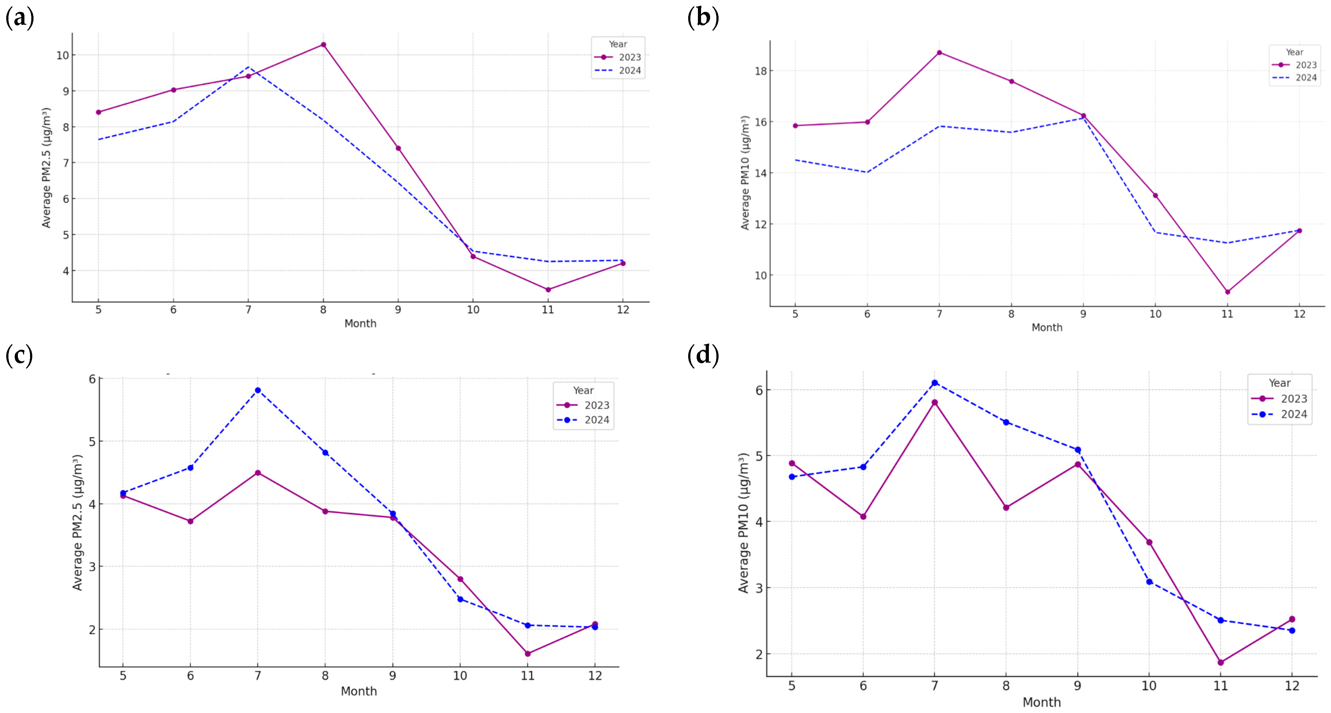
Trend analysis has been performed on pollutant attributes (PM2.5 and PM10) to study temporal features of the data. Figure 4 depicts the average monthly trend of pollutants across the months of May (month 5) to December (month 12) for 2023 and 2024. At both locations, PM2.5 and PM10 levels appear to be higher in the colder months. These are typically the winter months (June to August) and early spring (September). This is likely due to increased residential heating (wood burning) and atmospheric conditions that trap pollutants near the surface.

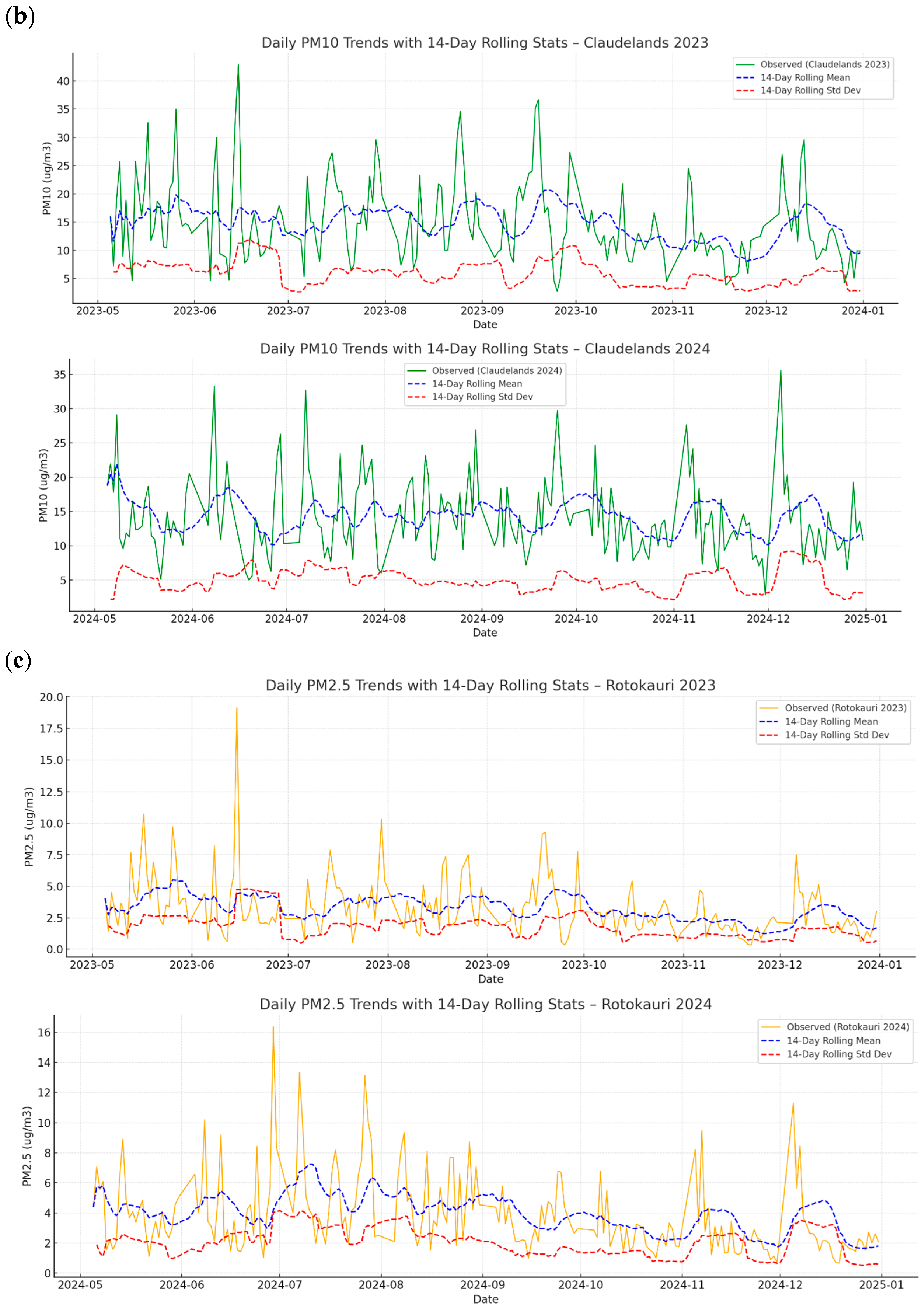
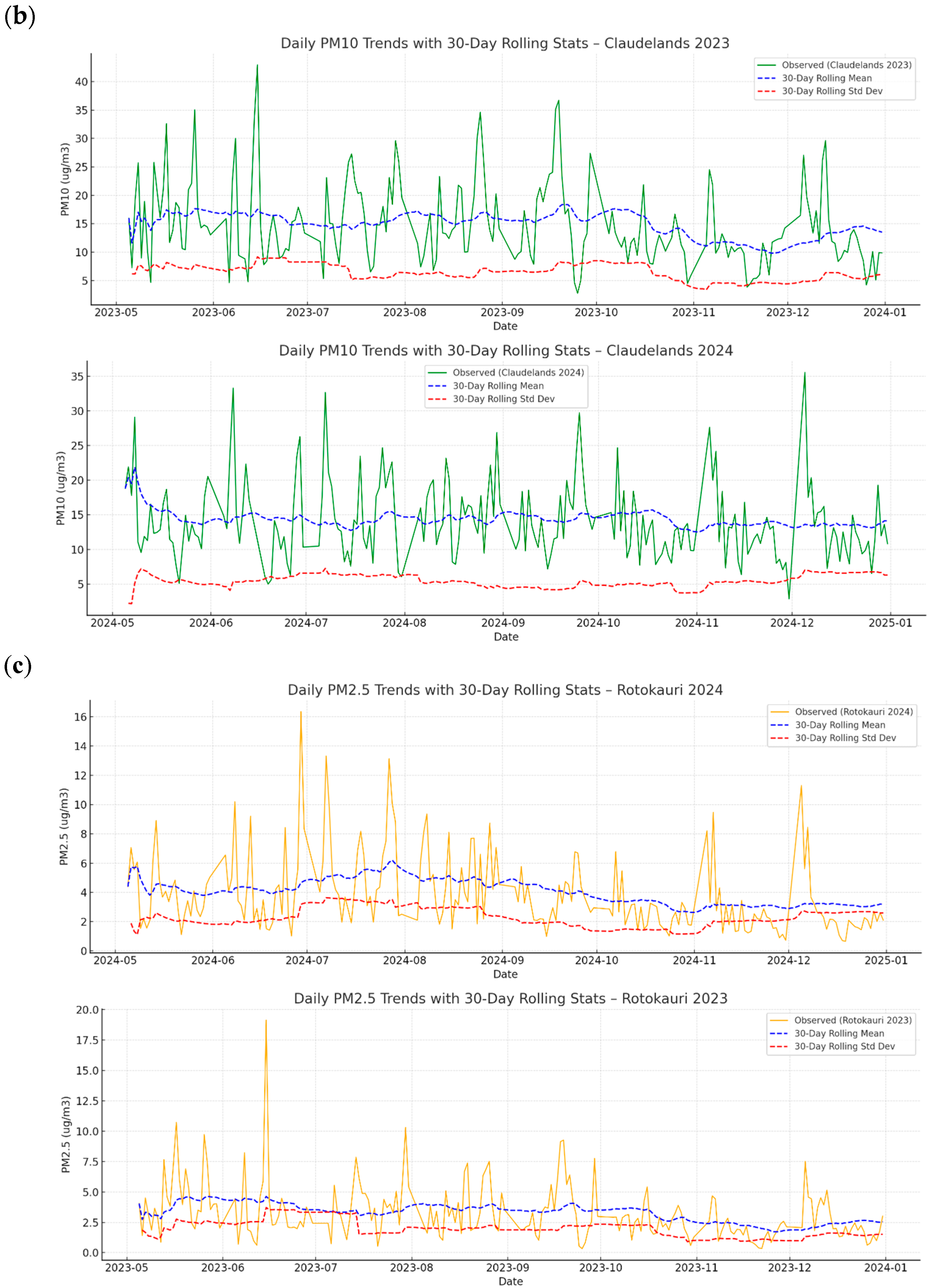
The 14-day rolling statistics in Figure 5 provide a finer temporal resolution, revealing intermittent pollution spikes which often exceed the seasonal baseline, which are likely linked to transient meteorological events such as calm, cold nights, or short-lived localised emissions. These fluctuations are particularly apparent at Claudelands, where wind speed data indicate that many short-term elevations coincide with reduced dispersion conditions. In contrast, the 30-day rolling statistics in Figure 6 smooth short-term variability to emphasise the broader seasonal cycle, clearly illustrating the winter crest and spring decay in both years. This longer window also allows a clearer comparison between years, with Claudelands showing a slightly sharper winter 2024 peak compared to 2023, suggesting possible interannual variability in emission intensity or meteorological conditions. At both sites, the winter-to-summer amplitude is substantial, which highlights a strong influence of seasonal heating and atmospheric stability on air quality. These multi-scale perspectives, such as monthly averages, 14-day rolling windows, and 30-day rolling windows, complement each other by enabling simultaneous identification of broad seasonal patterns and detection of short-lived anomalies, offering a more complete understanding of pollutant behaviour across time.

A more detailed view of pollutant data and trends is shown in Figure 5 and Figure 6, which together illustrate short-term versus long-term dynamics. Figure 5 presents the 14-day rolling statistics (mean and standard deviation), highlighting temporary fluctuations and pollution spikes associated with specific meteorological events or localised emissions. In contrast, Figure 6 shows the 30-day rolling statistics, which smooth short-term noise and emphasise broader seasonal cycles. This dual perspective is important, as the shorter window allows identification of episodic events (for example, winter inversion nights), while the longer window enables clearer comparisons across years and between sites. Both locations exhibit marked seasonal variation, with higher concentrations during winter months. As expected, pollutant levels at Rotokauri are generally lower than Claudelands, reflecting its more suburban and rural character with fewer traffic and heating sources.

3.2. Insights from Correlation Analysis

The statistical Pearson correlation matrix (linear correlation) for Claudelands and Rotokauri is shown in Figure 6. At Claudelands, particulate pollutants (PM2.5 and PM10) are strongly correlated with each other, but only weakly or slightly negatively correlated with meteorological factors such as temperature, wind speed, and wind direction. Similar correlations exist at Rotokauri. Strong correlations between PM1, PM2.5, and PM10 are not surprising because they largely come from the same emission sources, and PM2.5 is physically a subset of PM10. When the data are averaged by day, these links become even clearer since short-term fluctuations are smoothed out. Correlations between particulate pollutants and meteorological factors, such as temperature and humidity, are weak or slightly negative.

As depicted in Figure 7, the correlation analysis was performed using the Pearson correlation matrices for pollutant concentrations and meteorological parameters at the two locations Claudelands and Rotokauri. As observed at the two locations, there is a consistent trend where PM2.5 and PM10 demonstrated strong positive correlation (r = 0.91 at Claudelands and r = 0.95 at Rotokauri). This can be inferred as the two attributes are influenced by similar environmental or emission sources. On the other hand, the temperature exhibits a moderate negative correlation with PM2.5 at both sites (r = −0.60 at Claudelands; r = −0.45 at Rotokauri), this indicates that higher temperatures could support atmospheric dispersion or reduced local emissions. This relationship was also reported in previous studies [47], where higher temperatures are linked with improved atmospheric dispersion and reduced accumulation of pollutants. Furthermore, as observed, this inverse trend is also evident with PM10, albeit slightly weaker. Considering other specific factors exist at Claudelands, such as wind speed, there is a moderate negative correlation between wind speed and PM2.5 (r = −0.34), and this supports the role of wind in reducing pollutants. On the flip side, this variable was not present or reported for Rotokauri. Lastly, while humidity shows negligible correlation with particulates at Claudelands, it demonstrates a weak but consistently positive relationship with PM values at Rotokauri (up to r = 0.12).

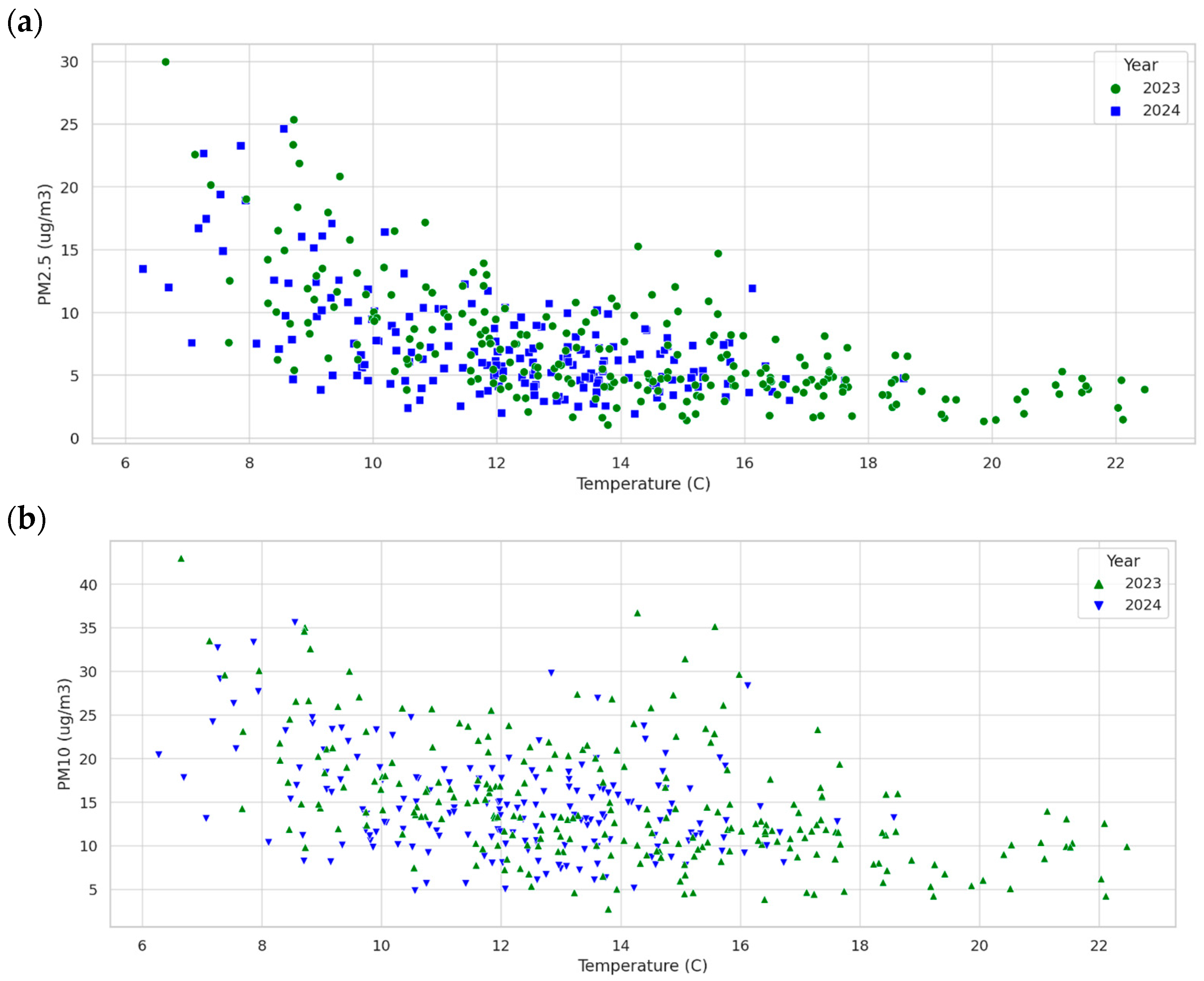
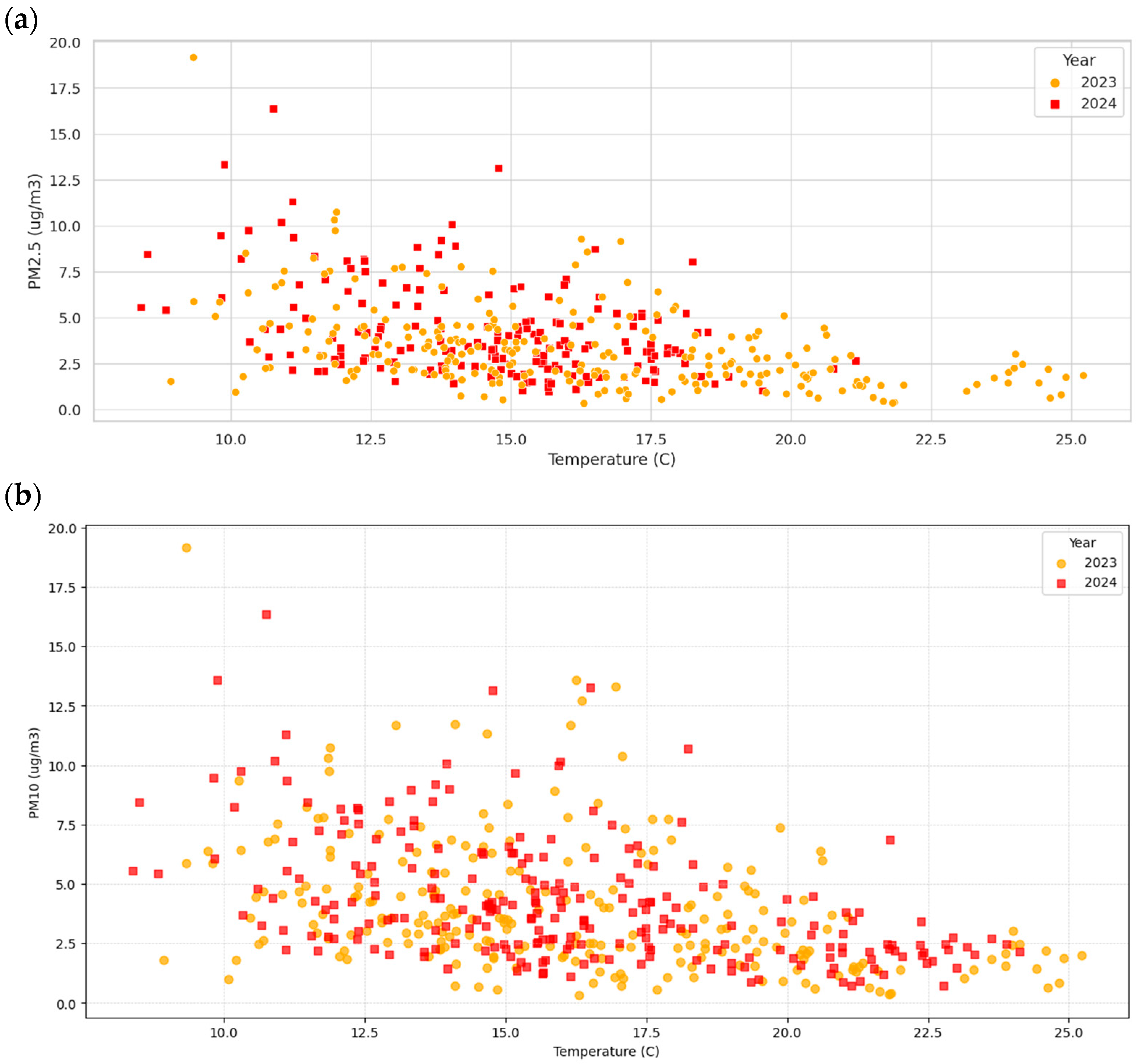
As outlined in Section 2.5, supervised learning has been performed using the common pollutant and meteorological attributes available at both locations. These are PM2.5, PM10, and air temperature. Figure 8 and Figure 9 illustrate the scatter plot relationship between the particulate matter pollutants and temperature. The slightly negative correlation between particulate matter pollutants and temperature is visible.

3.3. Unsupervised Learning

Unsupervised learning with the k-means clustering algorithm has been performed to determine clusters for the combination of pollutant and meteorological attributes at each air quality monitoring location. Figure 10 illustrates the optimal number of clusters determined using the elbow method. Three clusters are optimal for both locations in this study. These clusters are employed as labels for the supervised machine learning models.

The air quality data attribute statistics for each cluster are summarised in

Table 5. Summary of combined data attribute statistics in each cluster.

Cluster	Cluster Description	PM2.5 Range	PM2.5 Mean	PM10 Range	PM10 Mean	Temp Range	Temp Mean	AQI Range	AQI Mean
0	Cluster 0 (very good air quality)	0.3–6.6	2.7	0.3–9.9	3.7	8.9–25.2	16.7	0.3–9.9	3.7
1	Cluster 1 (good air quality)	2.1–13.3	6.1	5.4–19.3	12.0	7.1–22.1	13.9	5.4–19.3	12.0
2	Cluster 2 (moderate air quality)	6.6–29.9	13.2	16.4–43.0	23.5	6.3–19.3	10.9	16.4–43.0	23.5

(more detailed information for each location is provided in

Table A2. Summary of Claudelands data attribute statistics in each cluster.

Cluster	Cluster Description	PM2.5 Range	PM2.5 Mean	PM10 Range	PM10 Mean	Temp Range	Temp Mean	AQI Range	AQI Mean
0	Cluster 0 (very good air quality)	1.0–7.0	4.0	2.7–14.9	9.7	8.7–22.5	15.7	2.7–14.9	9.7
1	Cluster 1 (good air quality)	4.8–13.6	7.9	10.3–26.1	16.3	6.7–19.3	12.4	10.3–26.1	16.3
2	Cluster 2 (moderate air quality)	8.1–29.9	15.7	20.4–43.0	26.6	6.3–16.1	10.2	20.4–43.0	26.6

and

Table A3. Summary of Rotokauri data attribute statistics in each cluster.

Cluster	Cluster Description	PM2.5 Range	PM2.5 Mean	PM10 Range	PM10 Mean	Temp Range	Temp Mean	AQI Range	AQI Mean
0	Cluster 0 (very good air quality)	0.3–3.7	2.0	0.3–3.8	2.3	8.9–25.2	17.4	0.3–3.8	2.3
1	Cluster 1 (good air quality)	2.4–7.5	4.4	3.8–7.6	5.3	8.4–21.8	14.9	3.8–7.6	5.3
2	Cluster 2 (moderate air quality)	5.2–19.2	8.5	7.7–19.2	10.0	8.5–18.2	13.5	7.7–19.2	10.0

). Based on the AQI statistics, each cluster has been given a corresponding air quality rating. The AQI values at both locations did not exceed the moderate range over the two-year period. Hence, the good AQI category, which is normally 0–50, has been split into two categories (very good and good). The k-means clustering algorithm did not create perfectly distinct clusters and there is a small overlap in the values (Figure 11). Cluster 0 represents very good air quality with low particulate matter pollutants and higher temperatures. Higher particulate matter pollutants and lower temperatures are depicted in Cluster 1. Cluster 2 represents good air quality with mid-range particulate matter pollutants and mid-high temperatures. As shown in Section 3.2, there is a slightly negative correlation between particulate matter pollutants and temperature. Figure 12 illustrates the AQI and temperature distribution per cluster.

Table 5, Figure 10, and Figure 11 indicate that the clusters determined from the combined location data are representative of each individual location. Hence, the combined location clusters can be used in a classification model trained on data from both locations.

3.4. Supervised Learning

For supervised learning, models were trained on Claudelands data and evaluated on Rotokauri data, which resulted in an approximate 80:20 split by record counts. No random shuffling was applied, as the intention was to assess cross-location transferability rather than random partitioning. The combined dataset consists of standardised common pollutant and meteorological attributes at both locations (PM2.5, PM10, temperature, and AQI) as described in Section 3.3. The model learns patterns and relationships from the input data (PM2.5, PM10, temperature, and AQI) and the known outputs (AQI clusters) using the training data. Test data are used to establish the confusion matrices (Figure 13) and determine the performance metrics (

Table 6. Performance metrics of the supervised learning models.

Model	Accuracy	Weighted Average Accuracy	Macro Average Accuracy	Cluster	Precision	Recall	F1-Score
Random forest	0.93	0.98	0.94	Very good	1.00	1.00	1.00
				Good	0.81	1.00	0.90
				Moderate	1.00	0.97	0.98
SVM	0.61	0.47	0.90	Very good	0.20	1.00	0.33
				Good	0.21	0.82	0.34
				Moderate	1.00	0.59	0.74
KNN	0.83	0.93	0.52	Very good	0.17	1.00	0.29
				Good	0.40	0.77	0.53
				Moderate	1.00	0.85	0.92
Decision tree	0.91	0.98	0.94	Very good	1.00	1.00	1.00
				Good	0.81	1.00	0.90
				Moderate	1.00	0.97	0.98

).

4. Discussion

Predicting outdoor air quality indices (AQI) and forecasting particulate matter concentrations (PM2.5 and PM10) has become increasingly feasible with the advancement of machine learning techniques. By combining historical data from two monitoring locations, this study was able to assess trends and anticipate spikes when PM levels exceeded thresholds set by local and regional councils. In this work, PM data from the Rotokauri site were forecast and compared against Hamilton City Council data from the Claudelands station. The statistical analysis incorporated PM1, PM2.5, PM10, temperature, and relative humidity.

Results are consistent with previous literature, showing weak or slightly negative correlations between particulate matter and meteorological variables such as temperature and relative humidity. Wind speed demonstrated a moderate negative correlation with PM2.5, suggesting its role in pollutant dispersion. Leveraging these relationships, the supervised learning models, particularly random forest and decision tree, were able to predict air quality categories with high accuracy, demonstrating their suitability for cross site generalisation and operational air quality management.

4.1. Unsupervised Learning and Cluster Profiles

The modelling results demonstrate that integrating unsupervised clustering with supervised classification offers a robust approach for understanding and predicting air quality dynamics. The k-means algorithm (k = 3; Figure 11 and Figure 12) identified natural groupings in the data without relying on predefined AQI categories, allowing the analysis to reflect site-specific conditions rather than imposed thresholds. This flexibility is particularly important in medium-sized cities such as Hamilton, where environmental conditions vary between monitoring locations.

The k-means clustering generated three distinct clusters at each site (Table 5 and Table A2 and Table A3). In Claudelands, Cluster 0 (very good) encompassed PM2.5 concentrations between 1.0 and 7.0 µg/m³ (mean = 4.0) and PM10 between 2.7 and 14.9 µg/m³ (mean = 9.7), with mean temperatures around 15.7 °C. Cluster 1 (good) exhibited slightly elevated pollutant levels (PM2.5 mean = 7.9 µg/m³, PM10 mean = 16.3 µg/m³), while Cluster 2 (moderate) captured the highest concentrations, reaching PM2.5 up to 29.9 µg/m³ and PM10 up to 43.0 µg/m³. Rotokauri followed a similar three-cluster structure, though with substantially lower values overall. In the very good category, PM2.5 was recorded as low as 0.3 µg/m³ (mean = 2.0) and PM10 around 2.3 µg/m³, reflecting its semi-urban character. Even in the moderate cluster, PM2.5 rarely exceeded 19.2 µg/m³; well below the urban site’s maximum. When data from both sites were combined, the three-tiered hierarchy remained, but pollutant ranges widened due to the integration of urban and semi-urban measurements. This reinforces that, while seasonal and overall pollution patterns are shared, the magnitude of exposure differs, likely due to variations in traffic density, heating activity, and local land use.

The means of cluster reveal a consistent urban–semi-urban gradient. In the moderate category, Claudelands recorded a PM10 mean of 26.6 µg/m³ compared to Rotokauri’s 10.0 µg/m³, indicating that peak particulate concentrations in the urban core can be more than twice those in remote areas. This gap has direct public health implications, suggesting that emission control measures and public advisories may need to be prioritised for Claudelands during colder months. Temperature differences also align with expected seasonal drivers. Both sites’ very good clusters averaged mid-teen temperatures, whereas higher-pollution clusters tended to occur during cooler periods, which is consistent with increased winter heating and atmospheric conditions that limit dispersion.

These clustering outcomes directly reinforce the temporal patterns observed in the trend analysis (Figure 4, Figure 5, Figure 6, Figure 7 and Figure 8). The moderate clusters correspond closely with the elevated winter and early spring peaks identified in the monthly and rolling average plots (Figure 4, Figure 5 and Figure 6), while the very good clusters align with the summer troughs. The slightly elevated good clusters occupy transitional periods during autumn and late spring, mirroring the gradual rise and fall in pollutant levels. Moreover, the temperature profiles of each cluster match the inverse PM–temperature relationships shown in the correlation matrices and scatter plots (Figure 7), highlighting the role of seasonal meteorology in driving the observed pollutant cycles.

4.2. Supervised Learning and Its Influence on Predictive Performance

Cluster assignments derived from Claudelands were used as target labels to train four supervised classifiers: decision tree (DT), random forest (RF), support vector machine (SVM), and k-nearest neighbours (KNN), which were then evaluated on unseen data from Rotokauri (refer to Table 6). The results show that RF and DT achieved the highest accuracies, both exceeding 90%, with RF marginally outperforming DT in precision. This aligns with RF’s ensemble nature, which reduces variance by averaging predictions from multiple decorrelated trees, enabling it to capture complex, non-linear feature interactions inherent in environmental datasets. DT, while less complex, proved effective due to its fit-for-purpose and suitability for small- to medium-sized datasets such as the one used here.

The results are particularly striking, where random forest (RF) achieved 93.6% accuracy with a precision of 93.6%, marginally outperforming decision tree (DT) at 91.8% accuracy and 93.6% precision. RF’s advantage reflects its ensemble design, which mitigates overfitting and captures subtle non-linear interactions, such as how PM2.5 and PM10 concentrations respond differently to changes in temperature and wind speed. The strong performance of DT, despite its simplicity, indicates that the cluster boundaries generated in the unsupervised stage were inherently effectively structured, requiring minimal complexity to classify accurately.

Support vector machine (SVM) and k-nearest neighbours (KNN) also achieved competitive but slightly lower performance, 61% and 83% accuracy, respectively, likely due to their sensitivity to shifts in feature space between urban and semi-urban environments. For KNN, variations in pollutant distribution density between Claudelands and Rotokauri could have altered nearest neighbour relationships, while SVM’s reduced performance suggests that some cluster boundaries were not perfectly linearly separable, particularly in transitional pollution states.

The fact that all four models maintained high predictive power across sites demonstrates that cluster-derived categories generalise effectively, even without domain-specific retraining. This finding has direct operational implications: instead of building site-specific models for every location, a single well-trained model could be deployed city-wide, extending predictive coverage to areas with only low-cost or limited sensors. For Hamilton, where continuous high-grade monitoring is scarce, this approach offers a scalable and cost-efficient path to comprehensive air quality forecasting.

However, the method’s success is linked to environmental comparability. In our dataset, both sites exhibited strong PM2.5–PM10 correlations (r > 0.92) and similar negative relationships between temperature and particulate levels, suggesting shared dominant emission sources: traffic, winter heating, and, during spring, pollen release from the hay fever season.

5. Conclusions and Future Directions

This study makes three key methodological contributions. First, it demonstrates the effectiveness of a two-stage machine learning pipeline, combining unsupervised k-means clustering with supervised classification for predicting air quality categories in a medium-sized city with limited monitoring infrastructure. Unlike traditional AQI prediction models that rely solely on labelled datasets, the clustering stage derives site-specific air quality groupings from the data itself, allowing for flexible adaptation to local environmental patterns without the need for large-scale annotation. By combining clustering with classification, the method reduces the reliance on large, labelled datasets and is therefore suited to cities where continuous multi-year data are unavailable.

Second, the approach uses daily averaging and rolling statistical windows to smooth short-term fluctuations and seasonal noise, stabilising model training and reducing overfitting risks. This is particularly relevant for Hamilton, where monitoring data are more fragmented, and pollutant concentrations show strong temporal variability influenced by winter heating and the hay fever season. The inclusion of PM1, PM2.5, and PM10 measurements alongside temperature and relative humidity enables the models to account for seasonal peaks in airborne particles such as pollen, which can exacerbate respiratory health issues even when AQI remains in the moderate range.

A novel element of this study is the demonstration that models trained on an urban station (Claudelands) can predict with high accuracy at a semi-urban station (Rotokauri). While this is a promising finding, further validation of this innovation requires additional variables such as NO₂, O₃, CO, and SO₂, and multi-year data to allow systematic comparison with published results. Expanding the feature set and temporal coverage will be a priority in future work.

In summary, the study validates cross-location applicability by training models on Claudelands data and testing them on Rotokauri. This transfer learning aspect shows that high accuracy (>90% for random forest and decision tree) can be achieved without retraining on every new site, greatly increasing the operational scalability of air quality prediction in regions with sparse monitoring coverage. A limitation of this study is the relatively short eight-month dataset, and future work will extend the analysis to multi-year records as more Rotokauri data become available to capture long-term seasonal and inter-annual variability.

References

1. Chimka, J.R.; Ozdemir, E.A. Proportional Odds Model of Particle Pollution. Environments 2014, 1, 54–59. [Google Scholar] [CrossRef]
2. Alvarez-Mendoza, C.I.; Teodoro, A.C.; Torres, N.; Vivanco, V. Assessment of Remote Sensing Data to Model PM10 Estimation in Cities with a Low Number of Air Quality Stations: A Case of Study in Quito, Ecuador. Environments 2019, 6, 85. [Google Scholar] [CrossRef]
3. Waikato Region-Air Quality. Land, Air, Water Aotearoa (LAWA). 2021. Available online: https://www.lawa.org.nz/explore-data/waikato-region/air-quality/ (accessed on 26 September 2021).
4. Fanger, P.O. What is IAQ? Indoor Air 2006, 16, 328–334. [Google Scholar] [CrossRef]
5. Boamponsem, L.K.; Hopke, P.K.; Davy, P.K. Long-term trends and source apportionment of fine particulate matter (PM2.5) and gaseous pollutants in Auckland, New Zealand. Atmos. Environ. 2024, 322, 120392. [Google Scholar] [CrossRef]
6. Ancelet, T.; Davy, P.K.; Trompetter, W.J.; Markwitz, A.; Weatherburn, D.C. Sources and transport of particulate matter on an hourly time-scale during the winter in a New Zealand urban valley. Urban Clim. 2014, 10, 644–655. [Google Scholar] [CrossRef]
7. Tian, X.; Lu, C.; Song, Z.; An, C.; Wan, S.; Peng, H.; Feng, Q.; Chen, Z. Quantifying weather-induced unreliable public transportation service in cold regions under future climate model scenarios. Sustain. Cities Soc. 2024, 113, 105660. [Google Scholar] [CrossRef]
8. Williams, K.; Jones, R.J.; Al-Rawi, M. Particulate matter (PM2.5) and mould characteristics in selected classrooms located in Waikato, New Zealand: Preliminary results. Environments 2023, 10, 182. [Google Scholar] [CrossRef]
9. Muthukumar, P.; Cocom, E.; Nagrecha, K.; Comer, D.; Burga, I.; Taub, J.; Calvert, C.F.; Holm, J.; Pourhomayoun, M. Predicting PM2.5 atmospheric air pollution using deep learning with meteorological data and ground-based observations and remote-sensing satellite big data. Air Qual. Atmos. Health 2021, 15, 1221–1234. [Google Scholar] [CrossRef] [PubMed]
10. Mathew, A.; Gokul, P.R.; Shekar, P.R.; Arunab, K.S.; Abdo, H.G.; Almohamad, H.; Dughairi, A.a.A. Air quality analysis and PM 2.5 modelling using machine learning techniques: A study of Hyderabad city in India. Cogent Eng. 2023, 10, 2243743. [Google Scholar] [CrossRef]
11. Adong, P.; Bainomugisha, E.; Okure, D.; Sserunjogi, R. Applying machine learning for large scale field calibration of low-cost PM2.5 and PM10 air pollution sensors. Appl. AI Lett. 2022, 3, e76. [Google Scholar] [CrossRef]
12. Tang, D.; Zhan, Y.; Yang, F. A review of machine learning for modeling air quality: Overlooked but important issues. Atmos. Res. 2024, 300, 107261. [Google Scholar] [CrossRef]
13. Ravindiran, G.; Hayder, G.; Kanagarathinam, K.; Alagumalai, A.; Sonne, C. Air quality prediction by machine learning models: A predictive study on the indian coastal city of Visakhapatnam. Chemosphere 2023, 338, 139518. [Google Scholar] [CrossRef]
14. Gupta, N.S.; Mohta, Y.; Heda, K.; Armaan, R.; Valarmathi, B.; Arulkumaran, G. Prediction of air quality Index using Machine Learning techniques: A Comparative analysis. J. Environ. Public Health 2023, 4916267. [Google Scholar] [CrossRef]
15. Senthivel, S.; Chidambaranathan, M. Machine Learning Approaches Used for Air Quality Forecast: A review. Rev. D Intell. Artif. 2022, 36, 73–78. [Google Scholar] [CrossRef]
16. Zhang, Z.; Zhang, S.; Chen, C.; Yuan, J. A systematic survey of air quality prediction based on deep learning. Alex. Eng. J. 2024, 93, 128–141. [Google Scholar] [CrossRef]
17. Huang, Y.; Ying, J.J.; Tseng, V.S. Spatio-attention embedded recurrent neural network for air quality prediction. Knowl.-Based Syst. 2021, 233, 107416. [Google Scholar] [CrossRef]
18. Huang, Y.; Yu, J.; Dai, X.; Huang, Z.; Li, Y. Air-Quality prediction based on the EMD–IPSO–LSTM combination model. Sustainability 2022, 14, 4889. [Google Scholar] [CrossRef]
19. Zaini, N.; Ean, L.W.; Ahmed, A.N.; Malek, M.A.; Chow, M.F. PM2.5 forecasting for an urban area based on deep learning and decomposition method. Sci. Rep. 2022, 12, 17565. [Google Scholar] [CrossRef]
20. Zhao, Z.; Wu, J.; Cai, F.; Zhang, S.; Wang, Y. A hybrid deep learning framework for air quality prediction with spatial autocorrelation during the COVID-19 pandemic. Sci. Rep. 2023, 13, 1015. [Google Scholar] [CrossRef]
21. Li, W.; Jiang, X. Prediction of air pollutant concentrations based on TCN-BiLSTM-DMAttention with STL decomposition. Sci. Rep. 2023, 13, 4665. [Google Scholar] [CrossRef]
22. Mohammadi, F.; Teiri, H.; Hajizadeh, Y.; Abdolahnejad, A.; Ebrahimi, A. Prediction of atmospheric PM2.5 level by machine learning techniques in Isfahan, Iran. Sci. Rep. 2024, 14, 2109. [Google Scholar] [CrossRef]
23. Vieru, M.; Cărbureanu, M. Machine Learning methods applied in air quality prediction. Rom. J. Pet. Gas Technol. 2024, 5, 5–18. [Google Scholar] [CrossRef]
24. Gladkova, E.; Saychenko, L. Applying machine learning techniques in air quality prediction. Transp. Res. Procedia 2022, 63, 1999–2006. [Google Scholar] [CrossRef]
25. Bai, X.; Zhang, N.; Cao, X.; Chen, W. Prediction of PM2.5 concentration based on a CNN-LSTM neural network algorithm. PeerJ 2024, 12, e17811. [Google Scholar] [CrossRef]
26. Bellinger, C.; Jabbar, M.S.M.; Zaïane, O.; Osornio-Vargas, A. A systematic review of data mining and machine learning for air pollution epidemiology. BMC Public Health 2017, 17, 907. [Google Scholar] [CrossRef]
27. Wood, D.A. Trend-attribute forecasting of hourly PM2.5 trends in fifteen cities of Central England applying optimized machine learning feature selection. J. Environ. Manag. 2024, 356, 120561. [Google Scholar] [CrossRef]
28. Gundogdu, S.; Elbir, T. Elevating hourly PM2.5 forecasting in Istanbul, Türkiye: Leveraging ERA5 reanalysis and genetic algorithms in a comparative machine learning model analysis. Chemosphere 2024, 364, 143096. [Google Scholar] [CrossRef]
29. Waikato Regional Council. (n.d.). Hamilton Airshed—Claudelands—Air Quality. Waikato Regional Council. Available online: https://www.waikatoregion.govt.nz/environment/envirohub/environmental-maps-and-data/station/967611/PM2.5?dt=PM+2.5 (accessed on 5 March 2025).
30. Al-Rawi, M.A.; Chand, P.; Evangelista, A.V.M. Cost-effective customizable indoor environmental quality monitoring system. Adv. Technol. Innov. 2022, 7, 1–14. [Google Scholar] [CrossRef]
31. OpenStreetMap Contributors. (n.d.). Node 60729033. OpenStreetMap. Available online: https://www.openstreetmap.org/node/60729033#map=14/-37.78788/175.28179 (accessed on 5 March 2025).
32. Environmental Health Intelligence New Zealand. Population Size and Change. Environmental Health Indicators New Zealand. 2023. Available online: https://www.ehinz.ac.nz/indicators/population-vulnerability/population-size-and-change/ (accessed on 15 July 2024).
33. Stats NZ. Hamilton City: Place and Ethnic Group Summaries. Stats NZ. Available online: https://tools.summaries.stats.govt.nz/places/TA/hamilton-city (accessed on 7 March 2025).
34. Ministry for the Environment (MfE) New Zealand’s Environmental Reporting Series: Our Air 2021. Available online: https://environment.govt.nz/publications/our-air-2021 (accessed on 7 March 2025).
35. U.S. Environmental Protection Agency (USEPA). Technical Assistance Document for the Reporting of Daily Air Quality. AirNow. 2024. Available online: https://www.airnow.gov/publications/air-quality-index/technical-assistance-document-for-reporting-the-daily-aqi/ (accessed on 23 July 2024).
36. Waskom, M.L. seaborn: Statistical data visualization. J. Open-Source Softw. 2021, 6, 3021. [Google Scholar] [CrossRef]
37. Lloyd, S. Least squares quantization in PCM. IEEE Trans. Inf. Theory 1982, 28, 129–137. [Google Scholar] [CrossRef]
38. Murphy, K.P. Machine Learning: A Probabilistic Perspective; MIT Press: Cambridge, MA, USA, 2012. [Google Scholar]
39. Breiman, L.; Friedman, J.H.; Olshen, R.A.; Stone, C.J. Classification and Regression Trees (CART); Wadsworth Brooks: New York, NY, USA, 1984. [Google Scholar]
40. Quinlan, J.R. Induction of Decision Trees. Mach. Learn. 1986, 1, 81–106. [Google Scholar] [CrossRef]
41. Pedregosa, F.; Varoquaux, G.; Gramfort, A.; Michel, V.; Thirion, B.; Grisel, O.; Blondel, M.; Prettenhofer, P.; Weiss, R.; Dubourg, V.; et al. Scikit-Learn: Machine Learning in Python. J. Mach. Learn. Res. 2011, 12, 2825–2830. Available online: http://jmlr.org/papers/v12/pedregosa11a.html (accessed on 1 August 2024).
42. Breiman, L. Random Forests. Mach. Learn. 2001, 45, 5–32. [Google Scholar] [CrossRef]
43. Cortes, C.; Vapnik, V. Support-Vector Networks. Mach. Learn. 1995, 20, 273–297. [Google Scholar] [CrossRef]
44. Cover, T.M.; Hart, P.E. Nearest neighbor pattern classification. IEEE Trans. Inf. Theory 1967, 13, 21–27. [Google Scholar] [CrossRef]
45. Ting, K.M. Confusion matrix. In Encyclopedia of Machine Learning; Sammut, C., Webb, G.I., Eds.; Springer: Greer, SC, USA, 2010; p. 209. [Google Scholar] [CrossRef]
46. Chand, P.; Assaf, M. An empirical study on lightweight CNN models for efficient classification of used electronic parts. Sustainability 2024, 16, 7607. [Google Scholar] [CrossRef]
47. Rahman, M.; Meng, L. Examining the Spatial and Temporal Variation of PM2.5 and Its Linkage with Meteorological Conditions in Dhaka, Bangladesh. Atmosphere 2024, 15, 1426. [Google Scholar] [CrossRef]
Figure 1. Workflow of two-stage machine learning framework air quality prediction in Hamilton, New Zealand.
Environments 12 00336 g001
Figure 2. Claudelands and Rotokauri air quality monitoring station locations in Hamilton city.
Environments 12 00336 g002
Figure 3. Evaluation metrics in a confusion matrix.
Environments 12 00336 g003
Figure 4. Average monthly trend analysis of PM2.5 and PM10 at Claudelands and Rotokauri; (a) Claudelands PM2.5 trend; (b) Claudelands PM10 trend; (c) Rotokauri PM2.5 trend; and (d) Rotokauri PM10 trend.
Environments 12 00336 g004
Figure 5. The 14-day rolling statistics of pollutant levels at Claudelands and Rotokauri; (a) Claudelands PM2.5 trend (2023 vs. 2024); (b) Claudelands PM10 trend (2023 vs. 2024); (c) Rotokauri PM2.5 trend (2023 vs. 2024); and (d) Rotokauri PM10 trend.
Environments 12 00336 g005aEnvironments 12 00336 g005bEnvironments 12 00336 g005c
Figure 6. The 30-day rolling statistics of pollutant levels at Claudelands and Rotokauri.; (a) Claudelands PM2.5 trend (2023 vs. 2024); (b) Claudelands PM10 trend (2023 vs. 2024); (c) Rotokauri PM2.5 trend (2023 vs. 2024); and (d) Rotokauri PM10 trend.
Environments 12 00336 g006aEnvironments 12 00336 g006bEnvironments 12 00336 g006c
Figure 7. Statistical Pearson correlation matrix (pollutant and meteorological variables); (a) Claudelands correlation matrix and (b) Rotokauri correlation matrix.
Environments 12 00336 g007
Figure 8. Claudelands scatter plot relationship between particulate matter pollutants and temperature; (a) PM2.5 and (b) PM10.
Environments 12 00336 g008
Figure 9. Rotokauri scatter plot relationship between particulate matter pollutants and temperature; (a) PM2.5 and (b) PM10.
Environments 12 00336 g009
Figure 10. Elbow method plots for k-means clustering; (a) Claudelands; (b) Rotokauri; and (c) combined.
Environments 12 00336 g010
Figure 11. AQI distribution in each cluster; (a) Claudelands; (b) Rotokauri; and (c) combined.
Environments 12 00336 g011
Figure 12. AQI and temperature distribution per cluster; (a) Claudelands; (b) Rotokauri; and (c) combined.
Environments 12 00336 g012
Figure 13. Confusion matrices of the supervised learning models. (a) Random Forest and SVM; (b) KNN and Decision Tree.
Environments 12 00336 g013