Inactivation of Continuously Released Airborne Virus by Upper-Room UVC LED Irradiation Under Realistic Testing Conditions

Abstract

Ultraviolet (UV) radiation can be used to inactivate microorganisms, with upper-room UV germicidal irradiation (UR-UVGI) representing a promising approach. This study investigated the inactivation of the airborne surrogate virus Phi6 by a UR-UVGI system based on light-emitting diodes (LEDs) in a realistic test setup. Two test scenarios were used, one with continuous Phi6 release, simulating a source located in the room and leading to a dynamic equilibrium, and the second simulating a situation in which the source has left the room and an exponential decay is evaluated. The “Incremental Evaluation Model” was adapted and used to evaluate the dynamic equilibrium measurement. At a position in the breathing direction 5 m away from the Phi6 source, the loss coefficient (air exchange rate) was 25 h⁻¹ in the first scenario and 30 h⁻¹ in the second. These results show that UR-UVGI systems can effectively inactivate microorganisms. However, at 1 m distance from the Phi6 source perpendicular to the breathing direction, only minimal inactivation was observed due to short-circuit airflow. At this position, the loss coefficient was <2 h⁻¹ in the first scenario and 17 h⁻¹ in the second scenario, indicating that short-circuit airflows can only be detected by dynamic equilibrium measurements.

1. Introduction

Since people in modern societies spend most of their lives indoors, the impact of indoor environment quality (IEQ) on people’s health should be considered. Aspects such as temperature and humidity, but also acoustics and light, influence people’s well-being. Released or infiltrated particles, gaseous pollutants, radon, allergens, and microorganisms can significantly impact indoor air quality (IAQ). Pathogenic microorganisms are of particular concern in hospitals, nursing homes, and generally during epidemics and pandemics. The need for healthy indoor air leads to the need for technical solutions to improve indoor air quality, since ventilation by opening windows and eliminating the source of the pollutant are not always an option. Filtration and adsorption technologies can remove all of the above-mentioned pollutants from the air. However, they have the disadvantage that the air to be cleaned must be passed through the cleaning unit. These technologies therefore require fans, and these are typically associated with noise. With microorganisms (e.g., bacteria, viruses, mold), the alternative is not to remove them from the air but to inactivate them while they are airborne in the room.

Ultraviolet germicidal irradiation, especially in the UVC range (200–280 nm), is a well-established method for disinfecting water [1], surfaces [2,3], and air. Fields of application of UVC are, for example, aircraft cabins. Belland et al. suggested that UVC radiation, maintained below the exposure limits, can be a valuable addition to existing measures against disease transmission during flights [4].

The utilization of ultraviolet irradiation of the whole interior below exposure limits is one possible way by which to inactivate microorganisms in the air and on surfaces [4,5]. Direct exposure to UVC radiation can cause harmful effects to humans, leading to eye damage, premature skin aging, and an increased risk of skin cancer, which restricts its application. The risk to human health from ultraviolet (UV) radiation (200–400 nm) has been discussed in the literature [4,6,7]. Additionally, certain materials may suffer damage from structural deterioration if exposed to UVC radiation for an extended period [8].

The use of UV radiation in the upper part of the interior is another possible way by which to inactivate airborne microorganisms without exposing people in the room to UV radiation [9,10,11,12,13,14,15,16,17,18,19,20,21,22,23,24,25,26,27,28,29,30,31,32,33,34,35,36,37,38,39,40,41,42]. These inactivating systems are called “upper space irradiation” [31], “upper room ultraviolet air disinfection” [41], “upper-room ultraviolet germicidal irradiation” (UR-UVGI) [9,12,19,20,23,24,35,36,42], “germicidal ultraviolet” (GUV) [10,26,38,39,40,43], or, in general, “upper room ultraviolet irradiation”. Furthermore, the term “upper air” has been used [16,17,44,45]. The microorganism inactivating system utilized for the investigations presented in this publication belongs to these “upper-room disinfection” or UR-UVGI systems and uses UVC radiation (280 nm) based on LED technology. It creates a thin radiation field aligned horizontally or parallel to the ceiling, also known as UVC carpet. The radiation inactivates microorganisms that fly through the radiation field.

The effect of inactivating microorganisms depends on various factors, such as organism-dependent resistance to UVC radiation [8]. The form in which the organism is present plays a role in whether, for example, droplets on surfaces or those that are airborne are protected as biofilms or as airborne particles. For the quantitative determination of fluence, for example, Kheyrandish et al. considered several correction factors for microbial inactivation studies [46]. The literature and the data regarding the inactivation of viruses in liquid media and on surfaces are plentiful, but it is complex to apply the same results to airborne microorganisms. The consistent results from liquids and surfaces can therefore not be transferred directly to airborne viruses [47]. The persistence (i.e., time-dependent infectivity) of microorganisms in the built environment determines the infection risk.

Particularly for enveloped viruses, including strains of influenza virus and SARS-CoV-2, the persistence of viruses in indoor environments, and therefore infectious disease transmission, is significantly influenced by environmental conditions, and particularly relative humidity (RH). RH has a greater impact on viral decay in larger droplets than in smaller droplets [47,48,49]. The effect of humidity on the natural loss of the infectivity of airborne Phi6, which has been used as a surrogate for influenza viruses and coronaviruses, follows a characteristic V-shaped curve, with the fastest natural loss at 75% and better resistance at other tested humidity levels at 25 °C [50]. The relative infectivity rate was 3 log lower, at 75% RH, than at 98% RH. However, temperature effects also have to be considered, as, at 14 °C and 19 °C, virus infectivity remained high across all of the RH tested. The increase in temperature to 37 °C, however, resulted in a further reduction in Phi6 infectivity by approximately 6 log and 2 log losses at 75% and 98% RH, respectively.

UVC radiation is absorbed by nucleic acids predominantly in the wavelength range between 250 and 270 nm, which leads to the formation of dimers (cyclobutane pyrimidine) and photoproducts (pyrimidine), modifying the DNA structure [51] and causing damage. At a wavelength of about 280 nm, UVC radiation is mainly absorbed by amino acids, in particular by tryptophan and tyrosine. This results in different germicidal effects, depending on the wavelength and sensitivity of bacteria, protozoa, viruses, and other microorganisms to ultraviolet radiation [52]. The UV inactivation of adenovirus, known for its high resistance to UV radiation, was more effectively achieved at 222 nm compared to 254 nm [53]. Inactivation at 222 nm was primarily influenced by damage to the capsid protein, indicating that UV radiation at this wavelength predominantly targets the capsid proteins of the adenovirus, whereas monochromatic UV at 254 nm primarily affects the genome.

Ultraviolet radiation at wavelengths below 242 nm interacts with oxygen, which can contribute to ozone (O₃) formation [54]. As an oxidant, it can react with gaseous components and material surfaces. Ozone can cause the formation of problematic by-products and affect health [55].

Ishida et al. evaluated the wavelength dependence of the inactivation effect from 250 to 300 nm and confirmed that the 267 nm LED has the highest inactivation effect on the bacterium E. coli [56].

Inagaki et al. investigated the inactivation of three variants of SARS-CoV-2 in 2021 using deep-ultraviolet radiation-emitting diode radiation (DUV-LED: 280 nm ± 5 nm) [57]. The plaque assay tests showed a relative reduction of the titer of a virus suspension of >90% after 1 s of continuous irradiation of the virus solution (3.75 mW/cm² at a distance of 20 mm). The diluted solution was applied to host cells. A 5-s continuous irradiation resulted in a reduction of ≥99.8% for each variant.

Takamure et al. aerosolized a virus suspension of a SARS-CoV-2 variant [58]. The aerosol was passed through an inactivation unit, and the aerosol was then collected on gelatine filters. An average loss rate of 53% of the viral aerosol was determined. The RNA reduction was 60% (4.8 mW/cm², 7.6 s, 36.5 mJ/cm²). The inactivation rate was ≥99.38%. In 2023, Takamure et al. published a reduction rate of ≥99.89% at 12.2 mJ/cm² [59].

In addition to the route of exposure, the number of particles encountered during exposure correlates with the severity and outcome of the disease in some infectious diseases (dose−response relationship). For determination of the infective viral dose (ID₅₀), tissue culture infectious dose (TCID 50), or plaque assay (plaque forming unit—PFU) are applied. Karmzadeh et al. compared several pathogens and listed influenza as one of the most contagious viruses with a very low infective dose of 0.6–3.0 TCID 50 (H2N2 strain) [60].

A requirement for a viral test aerosol in real-scale test rooms, which are intended to represent a classroom or a meeting room, for example, is that it needs to be classified as non-pathogenic to humans. Bacteriophages are different groups of viruses that are specialized to infect bacteria as solely host cells. These viruses serve as surrogates for a pathogen of interest and should closely resemble it in terms of size and characteristic properties. Turgeon et al. assessed the suitability of selected bacteriophages as surrogates for several human and animal viruses [61]. For microbiological analysis, a bacteriophage plaque assay can be applied to determine the inactivation effectivity of air purification technologies. Moreover, the cultivation of bacteria is less demanding and less sensitive than animal or human cell cultures.

This publication presents the investigation of the inactivation of bacteriophage Phi6 using a UR-UVGI system to implement two test scenarios in a real-scale room. In the first scenario, continuous Phi6 release with the UVC radiation source switched on leads to a dynamic equilibrium. In the second scenario, Phi6 release is stopped before the UVC radiation is switched on, and the exponential concentration decline is analyzed.

The aim of the study was to demonstrate the inactivation of airborne viral aerosol using an upper-room air purifier based on UVC inactivation in a test room. The room was equipped with thermal manikins, tables, and chairs to simulate the situation in a meeting room. Furthermore, the wall surfaces were partially cooled to simulate cold window surfaces and to stimulate natural convection.

2. Materials and Methods

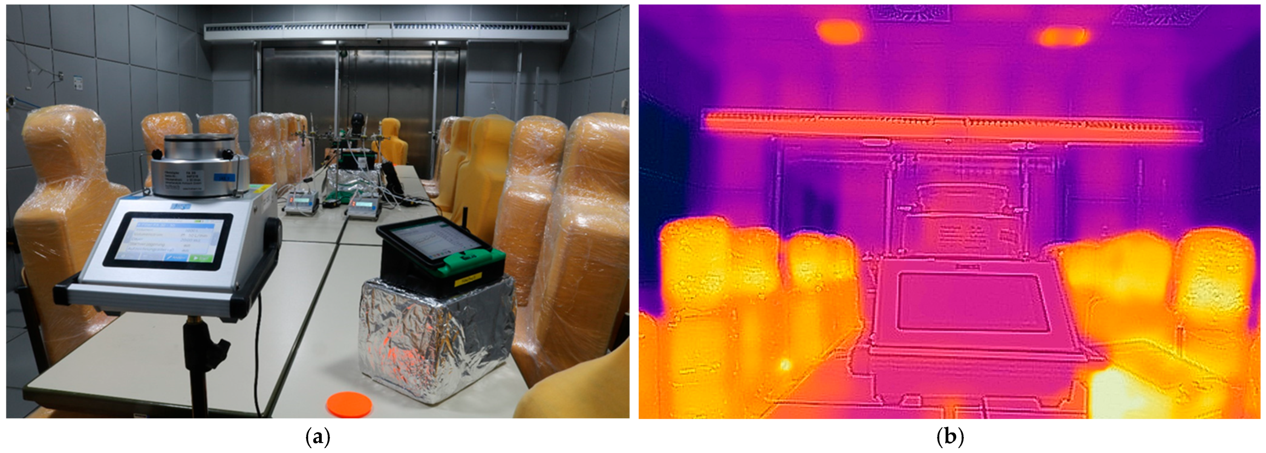
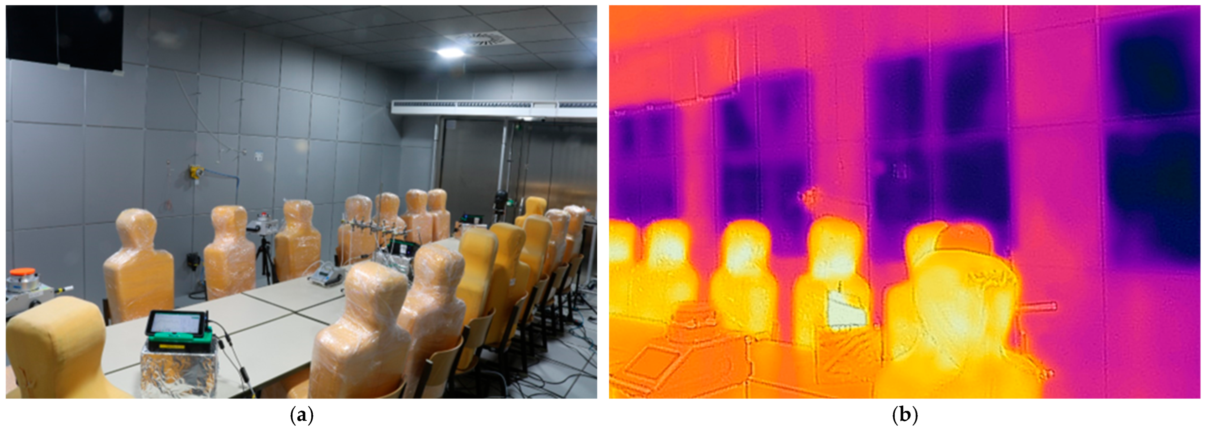
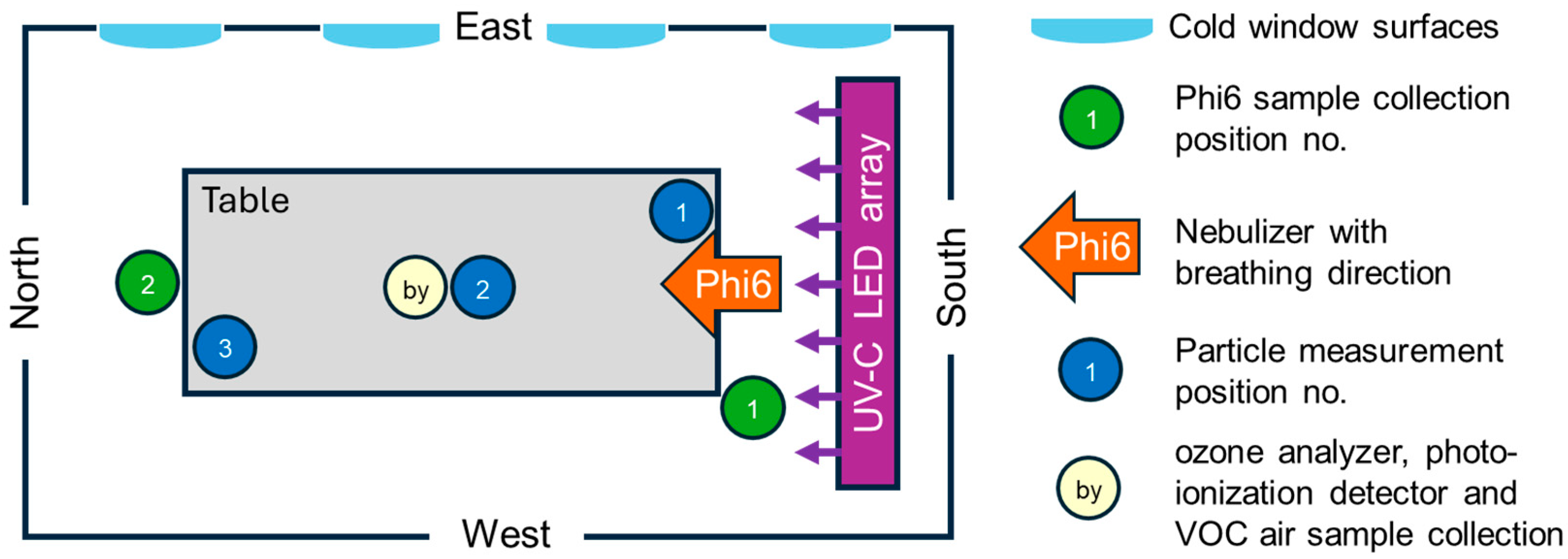
2.1. Test Room and Setup

The test of the UR-GUVI system was conducted in the Fraunhofer Indoor Air Test Center (IATC) in Valley, Germany (Figure 1 and Figure 2). The IATC is a test facility with a room volume of 129 m³ (8.24 × 5.06 × 3.09 m³), in which the climatic conditions during the measurement period are specifically set and kept constant. The test room was equipped with chairs, tables, and thermal manikins to simulate the situation and thermal conditions in a meeting room. A test room with a high ceiling was selected in order to keep the distance for vertical circulation long on the one hand but within the usual range on the other. Phi6 bacteriophages remain biologically active for longer in environments with lower humidity, so a humidity level between 30 and 50% was chosen.

The setup, including the Phi6 air sample collection positions and the particle measurement positions, is shown schematically in Figure 3.

The heat load of each thermal manikin was set to 78 W. This corresponds to the usual heat load generated by a person [62]. The heat loss coefficient was 7.5 K/(78 W/1.8 m²) = 0.173 (m² K)/W. This corresponds to 1.1 CLO (1 CLO = 0.155 (K m²)/W) and thus to a moderate thermal insulation (e.g., using everyday winter clothing including underwear, shirt, pants, jacket, socks, and shoes). The thermal plume from a manikin without breathing function shows many similarities in the average flow field above the head to that induced by a real person. Simulation studies by Sankaran et al. resulted in a maximum vertical velocity of 0.17 m/s for the real person and 0.23 m/s for a thermal manikin with a heat load of 80 W [62].

Table 1. Surface temperatures and flow velocities at several positions in the test room.

Location in the Test room	Surface Temperature [°C]	Flow Velocity [m/s]
east wall	21	0.06–0.13
“windows” (cooled segments on east wall)	17.5	0.15–0.30
west wall	21	0.06–0.12
north wall	23	0.50–0.60
south wall	23	0.05–0.07
ceiling	23	-
floor	23	-
Thermal manikins on the north side	≈30	0.14–0.19
Thermal manikins on the east side	≈30	0.10–0.18
Thermal manikins on the south side	≈30	0.10–0.18
“breathing” Sheffield-Head (south side)	≈23	0.48–1.00
UVC LED radiation module (south side)	-	0.18–0.20

summarizes the surface temperatures and flow velocities at several positions in the test room. The flow velocities were determined at a height of 1.25 m and at a distance of approximately 15 cm from the surface in question. For the thermal manikins, measurements were performed in front of the heads.

The selected control variables ensured that the heat emitted from the thermal manikins, the measurement devices, and the UR-UVGI system, totaling 1900 W, could be dissipated, with the UR-UVGI system contributing 216 W (11%) and the 17 thermal manikins 1326 W (70%) of the heat output. This resulted in the following indoor climate conditions:

• Indoor air temperature: 22.5 °C (±0.5 K)
• Relative humidity: 39% (±5%) for the dynamic equilibrium measurement and 32% (±5%) for the exponential decay measurement
• Air pressure 947 mbar
• Air exchange rate 0 h⁻¹ (static, no air exchange applied in the test facility)

Horizontal air currents caused by people moving or breathing were not taken into account in the test setup. In reality, people do not sit motionless in their chairs for hours on end. The thermal plume above a manikin results in a volume flow of approximately 1.5 m³/min (0.25 m² × 6 m/min). The volume flow during a breath stroke of the Sheffield head was 0.0063 m³/min, which was approximately 240 times smaller than the volume flow due to the thermal plume. The influence of these effects on the cleaning performance of the UR-UVGI system would have to be determined using computer simulations (or by further experiments).

2.2. Materials, Equipment, and Methods

The investigations on aerosols in the air were carried out in accordance with VDI-EE 4300 Sheet 14 [63] and considering ANSI/AHAM AC-1:2020 [64] to determine the inactivation of biologically active viruses.

The present study utilized Pseudomonas phage Phi6 (DSM 21518; Leibniz Institute DSMZ-German Collection of Microorganisms and Cell Cultures GmbH; Braunschweig, Germany), an 85 nm enveloped double-stranded RNA (dsRNA) virus, as a coronavirus surrogate due to its morphological features [50,61,65,66]. Bacteriophage Phi6 has a phospholipid bilayer envelope with spike glycoproteins, which are similar to those of enveloped viruses (SARS-CoV-2, influenza virus, etc.). Phi6 is also a Biosafety Level 1 agent and thus is frequently used as a surrogate for pathogens [1,2,51,67]. It is a bacteriophage that infects the Gram-negative bacterium Pseudomonas sp. Plaque assay can be applied as the detection method due to the lytic life cycle of the selected bacteriophage. Detection of RNA can be used to quantify virus load, but plaque assay is needed to quantify the concentration of biologically active phages to determine the inactivation effect.

A nebulizer (AGK 2000, Palas GmbH, Karlsruhe, Germany) was combined with a Sheffield head and nebulized the bioaerosol at an inlet pressure of 1.5 bar. The Sheffield head, or the “breathing head”, had a ventilation rate of 9 strokes/min (breath frequency) and exhaled 0.7 L/stroke (tidal volume) into the room. This resulted in a minute ventilation of 6.3 L/min, which corresponds to the breathing of a person at rest. Typically, minute ventilation is equal to or higher than this value [68]. Each stroke consisted of 3.3 s of inhalation and 3.3 s of exhalation, with no pauses in between.

The nebulized liquid was a bacteriophage suspension according to AHAM AC-5-2022 [69]. The molar concentrations of the salts in the suspension were: 86 mM NaCl, 49 mM Na₂HPO₄, 22 mM KH₂PO₄, 1 mM CaCl₂, and 1 mM MgSO₄. The suspension was continuously mixed in the liquid reservoir to ensure a constant concentration of Phi6 virus in the aerosol.

The airborne phages were collected from the room air in accordance with DIN-ISO 16000-16 [70]. The filters were processed in accordance with DIN ISO 16000-17 [71]. Air samples for the plaque assays were collected by two Holbach air samplers (MBASS30V3-FA30, Umweltanalytik Holbach GmbH, Wadern, Germany) on gelatine membrane filters (Sartorius AG, Göttingen, Germany). For the measurements with continuous Phi6 release, 1 m³ of indoor air was collected within 20 min for each sample. During the exponential decay, an air volume of 0.4 m³ was collected within 8 min for each sample.

The amount of active surrogate viruses in the air samples was determined using the plaque assay method [72,73]. The plaque assay with Pseudomonas phage Phi6 (DSM 21518) was implemented in combination with host bacterium strain Pseudomonas sp. (DSM 21482). The analysis using plaque assay was based on DIN EN 13610 [73]. Gelatine filters were suspended in 10 mL of 37 °C phage buffer and diluted decadically. The obtained dilution levels (10⁰, 10⁻¹, 10⁻² for 0.4 m³ and 10⁰, 10⁻¹, 10⁻², 10⁻³ for 1 m³ sample volume) were used in four aliquots for plaque assays. The lower detection limit of the plaque assay analysis was 25 PFU/m³ for 1 m³ air samples and 63 PFU/m³ for 0.4 m³ air samples. We used plates with at least 10 or more plaques for determination. According to DIN EN 13610 (for the phage P008), only plaque counts that are less than 300 pfu/plate can be used. Therefore, in a conservative assumption of a maximum density of 100 pfu per plate, the upper limit of quantification was 2.5 × 10⁶ PFU/m³ for 0.4 m³ air samples and 10⁷ PFU/m³ for 1 m³ air samples. Hence, a wide range of concentrations can be covered when using the filtration method. The cleaning of the room before each test ensured that the viral background was below the detection limit.

The aerosols were measured in accordance with the specifications of VDI-EE 4300 Sheet 14 [63] at three different positions in the room by three identical light scattering aerosol spectrometers (LSAS; Fidas Frog, Palas GmbH, Karlsruhe, Germany) in the range of 0.18–20 µm. The aerosol spectrometers continuously recorded PM fractions (PM₁, PM_2.5, and PM₁₀) and the particle number concentration.

In accordance with the specifications of the German Federal Environment Agency, the determination of by-products generated during operation is required when using potentially ozone-producing air purification processes (UVC, plasma technology, ozone direct injection) [63]. These samples were obtained using Tenax TA^® adsorption tubes (Markes International GmbH, Offenbach am Main, Germany) for the detection of volatile organic compounds (VOCs) and very volatile organic compounds (VVOCs), analyzed using thermal desorption gas chromatography-mass spectrometry [74], and on DNPH cartridges for the determination of selected ketones and aldehydes, analyzed using the high-performance liquid chromatography-diode array detection method [75].

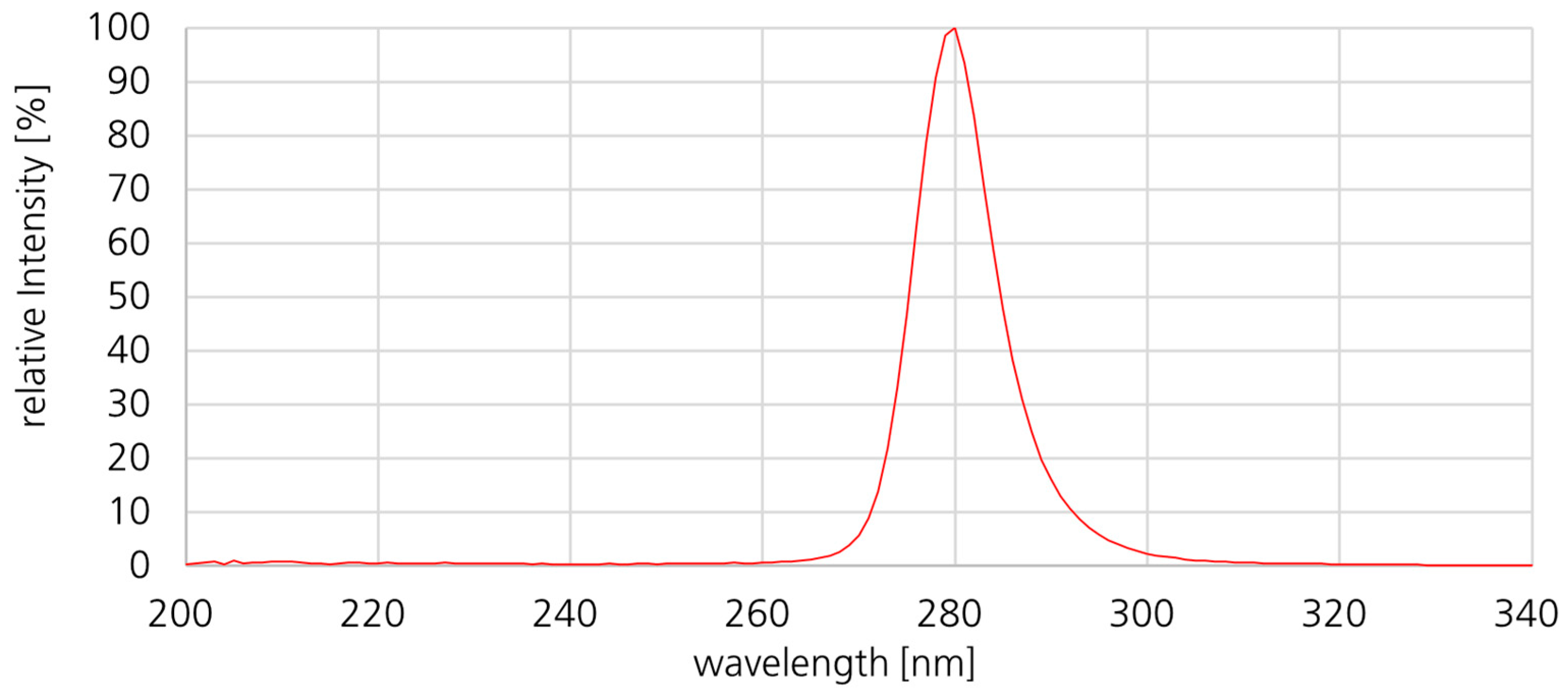
2.3. Description of the Investigated Upper-Room UVC Irradiation System

The used microorganism inactivating system belongs to the “upper-room disinfection” or “upper-room ultraviolet germicidal irradiation” (UR-UVGI) systems. The installed system had a length of 4.89 m and was mounted at a distance of 0.4 m from the south wall at a height of 2.5 m. It was based on LED technology and utilized UVC radiation. The LED array created a thin radiation field aligned horizontally or parallel to the ceiling, also known as a UVC carpet.

In UR-UVGI systems, the radiation inactivates microorganisms that are transported through the radiation field. In combination with the UVC LED technology, an extremely collimating optical system was utilized. Several optical units were positioned next to each other. The horizontal beam angle was negligible, at least in the central area of the device, because it was compensated for by the overlapping neighboring optical units. Due to the horizontal spread of the UVC radiation at an angle of around 4.5°, an overlap was achieved after just a few centimeters. This resulted in a closed radiation field with a vertical beam divergence of approximately ±2°. The widening of the radiation carpet led to a reduction in radiant intensity that was approximately proportional to the distance from the source. Due to the low divergence angle and in contrast to a point source, where the irradiance decreases with the distance to the source in the distance square, the irradiance of the used system remains high over large distances. Therefore, the system had an inactivating effect that extended far into the room. The used optical arrangement is a patented system [76].

In the test setup, 20 actively cooled NCSU434C LEDs from NICHIA Corporation (Anan, Tokushima 774-8601, Japan) were used. The LEDs were operated at 3 W and at a wavelength of 280 nm. The wavelength half-width of the emission peak was 10 nm. The emission spectrum of the LED is shown in Figure 4. In the operating state, an LED efficiency of approximately 5.6% could be assumed. The collimating optical system resulted in low losses, so that around 80–85% of the generated optical radiation left the system.

UR-UVGI systems utilize the natural convection in the room. The rising and the descending air traverse the UVC carpet, whereby the radiation inactivates airborne microorganisms, ideally after a single passage. Since the system utilizes the thermal air movement present in the room instead of circulating the air with fans, the system works without moving parts, except for small cooling fans. As a result, the technology operates almost noiselessly.

Adults emit approximately 80 W of heat energy into the room, which results in a typical air velocity between 0.04 and 0.20 m/s above people [62]. The inactivation dose corresponds to the irradiance multiplied by the dwell time in the irradiated area. The wider the radiation carpet, the longer the stay in this carpet. Therefore, the decline of the irradiance due to the widening of the beam is compensated by the increasing dwell time. At 1 m in front of the device, an average irradiance of approximately 10 W/m² can be measured in a 10 cm wide strip. An average vertical air flow of 5 cm/s corresponds to a dwell time of 2 s and thus a dose of 20 J/m² (=2 mJ/cm²) for a single vertical passage. For aerosols that cross the UVC carpet at an angle, the dose increases accordingly. If the entire ceiling is irradiated, the airborne microorganisms that sink back down are irradiated again.

If there are more people in the room, the heat output increases accordingly, and with it the vertical air movement in the room. The higher the vertical air movement, the more aerosols enter the UVC carpet, which corresponds to a higher equivalent air circulation rate.

2.4. Implementation of the Investigations (Time Schedule, Ventilation)

The schedule of the testing procedure with continuous Phi6 release (dynamic equilibrium) is described in

Table 2. Events during the determination of loss coefficient of the UR-UVGI system with Phi6 release during measurement (dynamic equilibrium).

Time of Day	tevent [h]	Event
08:30	−0.50	Start of particle measurement
08:30	−0.50	UR-UVGI system was switched on.
09:00	0.00	Aerosol release was switched on. (0 min)
09:16	0.27	Collection of first air sample until 09:36.
10:00	1.00	Collection of second air sample until 10:20.
10:21	1.35	UR-UVGI system was switched off.
10:46	1.77	Collection of third air sample until 11:05.
11:31	2.52	Collection of fourth air sample until 11:51.
11:53	1.88	Aerosol release was switched off. (173 min)
13:50	4.83	End of particle measurement

.

The schedule of the testing procedure without continuous Phi6 release (exponential decay) is described in

Table 3. Events during the determination of loss coefficient of an UR-UVGI system without Phi6 release during measurement (exponential decay).

Time of Day	tevent [h]	Event
08:26	−0.57	Start of particle measurement
08:29	−0.52	Start of air mixing (two fans oriented against each other)
09:00	0.00	Aerosol release was switched on (0 min)
09:50	0.83	End of air mixing
10:00	1.00	Aerosol release was switched off (60 min)
10:00	1.00	UR-UVGI system was switched on.
10:04	1.07	Collection of first air sample until 10:12.
10:12	1.20	Collection of second air sample until 10:20.
10:22	1.37	UR-UVGI system was switched off.
10:22	1.37	Start of air mixing (two fans oriented against each other)
10:22	1.37	Aerosol release was switched on (82 min)
11:12	2.20	End of air mixing (132 min)
11:22	2.37	Aerosol release was switched off (142 min)
11:26	2.43	Collection of third air sample until 11:34.
11:34	2.57	Collection of fourth air sample until 11:52.
13:24	4.40	End of particle measurement

.

There was no supply or exhaust air in the test room during the measurement, and the room air was not mechanically mixed (apart from the fans used to cool the LEDs). Only thermal convection caused by heat sources (thermal manikins, measurement equipment) and heat sinks (cold walls) led to (mainly vertical) air currents. During the dosing phases, the breathing head caused a weak horizontal airflow. There was a time delay of 4 min in the increase in particle concentration at position 3 (blue dot no. 3 in Figure 3), which corresponds to an average velocity of 0.02 m/s. This means that the horizontal flow velocity was 2.5 to 30 times lower than the measured vertical flow velocities (Table 1). Before measuring the exponential decline, the air in the room was mixed with fans for 50 min during the Phi6 release (60 min). To allow the thermal convection flow conditions to re-establish themselves prior to the measurement, the fans were switched off 10 min before the start of the exponential decline.

2.5. General Considerations on Modeling the Concentration Profiles for Continuous Phi6 Release

The Incremental Evaluation Model [77] can be used to mathematically describe first-order processes, in particular location-specific concentration profiles. A first-order process means that the change in concentration is proportional to the concentration itself. This requirement is met for the following investigations. In the model, the concentration approaches a steady state (or zero) as time t approaches infinity. In the steady state, the loss term equals the source term. The loss term is in turn calculated from the product of the concentration c and the loss coefficient k. In the model, the loss coefficient k is also an exponent (e^−kt). The loss coefficient therefore influences not only the equilibrium concentration, but also the time required to reach this equilibrium. In most cases, conditions change before a steady state is reached. The actual concentration at the time of the change is then the starting concentration for the next time increment (t_n < t < t_n+1). In its general form, this model is valid for all first-order processes. By adapting the model to specific requirements, the number of degrees of freedom can be reduced as needed. Whether the selected boundary conditions have been chosen appropriately must be checked on a case-by-case basis. Special care must be taken when selecting the time increments and designing the function of the source term s(t). For example, the source term can be constant or a function of time.

The evaluation process for the measurements performed with continuous Phi6 release is described below:

The determination of the natural Phi6 loss coefficient k_Nat (effect without UVC radiation) and the inactivation Phi6 loss coefficient k_AC (effect of UVC radiation) was divided into two steps. In the first step, the natural loss coefficient was determined together with two concentration parameters (the steady-state concentrations with and without UVC radiation). By varying the value of k_Nat, the curvature of the concentration profile was adjusted so that the profile passes through both sampling points during the measurement phase without UVC radiation (t > 81 min). In the second step, the parameter k_AC was determined by an equation that describes the steady-state condition (for time t towards infinity). It is important to clearly distinguish between these two steps. In the first step, a time-dependent process was evaluated, whereas in the second calculation step, time is irrelevant because the concentrations no longer change in the state under consideration due to the steady-state conditions.

Under ideal, well-mixed conditions, the concentration and thus the source term of active Phi6 phages is the same at every location in the test room. However, in the setup used for continuous Phi6 release measurements (Table 2 and Section 3.1), the room air was not moved by fans or other mechanical methods, so rapid horizontal mixing could not be ensured. Basically, the mixing (assumed mixing time: 12 min or 0.2 h) competes with the concentration loss (loss coefficient multiplied with concentration). In principle, three ranges can be distinguished:

• The process is dominated by the mixing. This condition applies to the aerosol loss coefficient. (k ≤ 0.2 h⁻¹ --> → e^−0.2×0.2 = e^−0.04 = 96%)
• The process is dominated by the loss term. This condition applies to the inactivation Phi6 loss coefficient. (k ≥ 20 h⁻¹ → e^−0.2×20 = e⁻⁴ = 2%)
• The process is influenced by both loss term and mixing. This condition applies to the natural Phi6 loss coefficient. (k ≅ 3.5 h⁻¹ → e^−0.2×3.5 = e^−0.7 = 50%)

With very low loss coefficients (range a), the concentration loss is negligible, and there is sufficient time to achieve good mixing in the room. In the investigations presented, it could be assumed that the aerosol was well mixed due to the very low aerosol loss coefficient (0.19 h⁻¹) and the resulting low concentration loss (Section 3.1.1 and Section 3.2.1). This assumption was supported by aerosol measurements at three positions in the test room. The aerosol consists mainly of salt solution droplets.

On the other hand, with very high loss coefficients (range b), the steady state can be achieved rapidly at a low concentration. The higher the loss coefficient, the faster concentration equilibrium is achieved. To model the concentration profile, it was assumed that the influx of active phages from the neighboring compartment does not immediately reach its equilibrium value. Instead, it was assumed that the establishment of the equilibrium of the source term can be characterized by the Phi6 loss coefficient as a rate constant. Since this model is based on a spatial concentration gradient, it is referred to as the gradient model. The released Phi6 phages were increasingly inactivated as they flew through the room, so that the concentration of active Phi6 phages could be lower at a location further away from the source than closer to the source. The higher the loss term (loss coefficient multiplied with concentration), the greater the spatial concentration gradient.

For loss coefficients between these two extremes (range c), the mathematical description becomes more difficult and less precise. This range potentially includes the natural Phi6 loss coefficients. For this publication, the calculation method for high loss coefficients was also used for the natural Phi6 loss coefficient (Section 3.1.2, Section 3.1.3, and Section 3.1.5). With this calculation method, a low loss coefficient results in an S-shaped concentration profile (Section 3.1.3 and Section 3.1.5). Alternatively, the natural loss coefficient can be determined using the well-mixed model (Section 3.1.4). In this model, the source term changes immediately when the source is switched (on or off). The well-mixed model tends to produce values for k_Nat that are too low, while the gradient model tends to produce values that are too high.

In the second step, the inactivation Phi6 loss coefficient k_AC is determined. Since the steady-state condition was used to calculate k_AC and no time effects were considered, only the spatial concentration gradient was relevant here. As with the determination of the parameter k_Nat, there is a choice between using the gradient model (Section 2.6.2) or the well-mixed model (Section 2.7.2). If the well-mixed model is used instead of the gradient model to determine the Phi6 inactivation loss coefficient, the effect of the inactivating system is overestimated, since the concentration is reduced partly due to the lower source term and not only due to the higher loss term.

2.6. Modeling for Continuous Phi6 Release in Combination with a Concentration Gradient

2.6.1. Calculation of Concentration Profile with Gradient Model

In a steady-state condition, the source term s [PFU/(m³ h)] equals the concentration loss [PFU/(m³ h)]. The concentration loss in the steady state is the product of the equilibrium concentration c_eq [PFU/m³] and the first-order total loss coefficient k_total [h⁻¹]. The steady-state condition is expressed by Equation (1):

$$\mathrm{s}={\mathrm{c}}_{\mathrm{e}\mathrm{q}}·{\mathrm{k}}_{\mathrm{t}\mathrm{o}\mathrm{t}\mathrm{a}\mathrm{l}}$$

(1)

Rearranging Equation (1) yields Equation (2), which is used for calculating the steady-state concentration c_ieq (at a specified position in the room) from the source term s_i [PFU/(m³ h)] and the loss coefficient k_i [h⁻¹]:

$${\mathrm{c}}_{\mathrm{i}\mathrm{e}\mathrm{q}}={\displaystyle \frac{{\mathrm{s}}_{\mathrm{i}}}{{\mathrm{k}}_{\mathrm{i}}}}$$

(2)

A modified version of the Incremental Evaluation Model [77] was used to evaluate the measurement with continuous aerosol release. Equation (3) describes the time t [h]-dependent concentration profile c(t) [e.g., PFU/m³] generally (in a specific place, if not well mixed). The equilibrium concentration c_eq [e.g., PFU/m³] is given by the ratio of the source term s(t) [e.g., PFU/(m³ h)] and the total loss coefficient k_total [h⁻¹]. Furthermore, the concentration c(t₀) [e.g., PFU/m³] at the beginning of the described part of the concentration profile is relevant.

$$\mathrm{c}\left(\mathrm{t}\right)={\displaystyle \frac{\mathrm{s}\left(\mathrm{t}\right)}{{\mathrm{k}}_{\mathrm{t}\mathrm{o}\mathrm{t}\mathrm{a}\mathrm{l}}}}+\left[\mathrm{c}\left({\mathrm{t}}_0\right)-{\displaystyle \frac{\mathrm{s}\left(\mathrm{t}\right)}{{\mathrm{k}}_{\mathrm{t}\mathrm{o}\mathrm{t}\mathrm{a}\mathrm{l}}}}\right]·{\mathrm{e}}^{-{\mathrm{k}}_{\mathrm{t}\mathrm{o}\mathrm{t}\mathrm{a}\mathrm{l}}·\left(\mathrm{t}-{\mathrm{t}}_0\right)} \mathrm{f}\mathrm{o}\mathrm{r} {\mathrm{t}}_0<\mathrm{t}<{\mathrm{t}}_1$$

(3)

Schumacher et al. described and utilized an equation that is comparable to Equation (3) [78].

The total loss coefficient k_total is the sum of all loss coefficients, which can be divided into the loss coefficient k_AC of the inactivating system and the loss coefficient k_Nat without the effect of the inactivating system. The parameter S is used as a switch to turn on or off the inactivating system in the formulas. Equation (4) is used for the further calculations.

$${\mathrm{k}}_{\mathrm{t}\mathrm{o}\mathrm{t}\mathrm{a}\mathrm{l}}={\mathrm{k}}_{\mathrm{N}\mathrm{a}\mathrm{t}}+\mathrm{S}·{\mathrm{k}}_{\mathrm{A}\mathrm{C}}$$

(4)

As the air in the test room was not well mixed, the spatio-temporal gradient of the source term s(t) [PFU/(m³ h)] must be considered for the measurements with continuous Phi6 release. Therefore, the source term, and hence the transitory equilibrium concentration at a specific position and a specific time, is not constant but a function of time.

Equation (5) describes the time t [h]-dependent source term profile s(t) [PFU/(m³ h)]. The equilibrium source term s_eq [PFU/(m³ h)] is reached in a steady state when t approaches infinity. Furthermore, the source term s(t₀) [PFU/(m³ h)] at the beginning of the described part of the source term profile is relevant.

$$\mathrm{s}\left(\mathrm{t}\right)={\mathrm{s}}_{\mathrm{e}\mathrm{q}}+\left[\mathrm{s}\left({\mathrm{t}}_0\right)-{\mathrm{s}}_{\mathrm{e}\mathrm{q}}\right]·{\mathrm{e}}^{-{\mathrm{k}}_{\mathrm{t}\mathrm{o}\mathrm{t}\mathrm{a}\mathrm{l}}·\left(\mathrm{t}-{\mathrm{t}}_0\right)} \mathrm{f}\mathrm{o}\mathrm{r} {\mathrm{t}}_0<\mathrm{t}<{\mathrm{t}}_1$$

(5)

To obtain the concentration profile, the curve was divided into time segments. In a specific time segment t_n+1 or (t_n+1 − t_n) [h], the transitory equilibrium concentration c_eq,n+1(t_n+1) [PFU/m³] is a function of the equilibrium concentration c_eq,n+1 [PFU/m³], the transitory equilibrium concentration c_eq,n(t_n) [PFU/m³] in the previous time segment, and the total loss coefficient k_total,n+1 [h⁻¹] that applies to the time segment t_n+1 or (t_n+1 − t_n) [h]; this is described by Equation (6).

$${\mathrm{c}}_{\mathrm{e}\mathrm{q},\mathrm{n}+1}\left({\mathrm{t}}_{\mathrm{n}+1}\right)={\mathrm{c}}_{\mathrm{e}\mathrm{q},\mathrm{n}+1}+\left({\mathrm{c}}_{\mathrm{e}\mathrm{q},\mathrm{n}}\left({\mathrm{t}}_{\mathrm{n}}\right)-{\mathrm{c}}_{\mathrm{e}\mathrm{q},\mathrm{n}+1}\right)·{\mathrm{e}}^{-{\mathrm{k}}_{\mathrm{t}\mathrm{o}\mathrm{t}\mathrm{a}\mathrm{l},\mathrm{n}+1}·\left({\mathrm{t}}_{\mathrm{n}+1}-{\mathrm{t}}_{\mathrm{n}}\right)}$$

(6)

In the time segment t_n+1 or (t_n+1 − t_n) [h], the concentration c_n+1(t_n+1) [PFU/m³] is a function of the transitory equilibrium concentration c_eq,n+1(t_n+1) [PFU/m³], the concentration c_n(t_n) [PFU/m³] in the previous time segment, and the total loss coefficient k_total,n+1 [h⁻¹] that applies to the time segment t_n+1 or (t_n+1 − t_n) [h]; this is described by Equation (7).

$${\mathrm{c}}_{\mathrm{n}+1}\left({\mathrm{t}}_{\mathrm{n}+1}\right)={\mathrm{c}}_{\mathrm{e}\mathrm{q},\mathrm{n}+1}\left({\mathrm{t}}_{\mathrm{n}+1}\right)+\left[{\mathrm{c}}_{\mathrm{n}}\left({\mathrm{t}}_{\mathrm{n}}\right)-{\mathrm{c}}_{\mathrm{e}\mathrm{q},\mathrm{n}+1}\left({\mathrm{t}}_{\mathrm{n}+1}\right)\right]·{\mathrm{e}}^{-{\mathrm{k}}_{\mathrm{t}\mathrm{o}\mathrm{t}\mathrm{a}\mathrm{l},\mathrm{n}+1}·\left({\mathrm{t}}_{\mathrm{n}+1}-{\mathrm{t}}_{\mathrm{n}}\right)}$$

(7)

The time step Δt = (t_n+1 − t_n) in the calculation of the concentration profile should be small enough that, for the expected k_total values, the condition exp(−k_total × Δt) ≅ (1 − k_total × Δt) is met. It is important to note that, for high total loss coefficients, the equilibrium concentration is reached within a few minutes; hence, the time resolution is not relevant if the sample is collected in the steady state. Therefore, either the product of k_total and Δt should be small enough (e.g., 6 h⁻¹ × 0.2 min/60 min/h = 0.02) or the steady state should be reached fast enough. The evaluation model was checked for time deviations in the applied range of the loss coefficients for time steps between 0.5 s and 5 min. For time steps of 1 min and lower no relevant influence of the time resolution was determined. The evaluation was carried out with time steps of 0.2 min.

2.6.2. Determination of k_AC Using the Gradient Model

The steady-state concentration c_1eq [PFU/m³], with source term s₁ [PFU/(h m³)] and loss coefficient k₁ = (k_Nat + k_AC) [h⁻¹] (inactivating system is active), is calculated by Equation (8):

$${\mathrm{c}}_{1\mathrm{e}\mathrm{q}}={\displaystyle \frac{{\mathrm{s}}_1}{{\mathrm{k}}_1}}={\displaystyle \frac{{\mathrm{s}}_1}{{\mathrm{k}}_{\mathrm{N}\mathrm{a}\mathrm{t}}+{\mathrm{k}}_{\mathrm{A}\mathrm{C}}}}$$

(8)

The steady-state concentration c_2eq [PFU/m³], with source term s₂ [PFU/(h m³)] and loss coefficient k₂ = k_Nat [h⁻¹] (inactivating system is not active), is calculated by Equation (9):

$${\mathrm{c}}_{2\mathrm{e}\mathrm{q}}={\displaystyle \frac{{\mathrm{s}}_2}{{\mathrm{k}}_{\mathrm{N}\mathrm{a}\mathrm{t}}}}$$

(9)

The ratio of the two steady-state concentrations c_2eq and c_1eq is described by Equation (10) or, after mathematical conversion, by Equation (11):

$${\displaystyle \frac{{\mathrm{c}}_{2\mathrm{e}\mathrm{q}}}{{\mathrm{c}}_{1\mathrm{e}\mathrm{q}}}}={\displaystyle \frac{\frac{{\mathrm{s}}_2}{{\mathrm{k}}_{\mathrm{N}\mathrm{a}\mathrm{t}}}}{\frac{{\mathrm{s}}_1}{{\mathrm{k}}_{\mathrm{N}\mathrm{a}\mathrm{t}}+{\mathrm{k}}_{\mathrm{A}\mathrm{C}}}}}$$

(10)

$${\displaystyle \frac{{\mathrm{c}}_{2\mathrm{e}\mathrm{q}}}{{\mathrm{c}}_{1\mathrm{e}\mathrm{q}}}}={\displaystyle \frac{{\mathrm{k}}_{\mathrm{N}\mathrm{a}\mathrm{t}}+{\mathrm{k}}_{\mathrm{A}\mathrm{C}}}{{\mathrm{k}}_{\mathrm{N}\mathrm{a}\mathrm{t}}}}·{\displaystyle \frac{{\mathrm{s}}_2}{{\mathrm{s}}_1}}$$

(11)

The ratio of the two equilibrium concentrations, c_2eq and c_1eq, yields the ratio factor F_R according to Equation (12):

$${\mathrm{F}}_{\mathrm{R}}={\displaystyle \frac{{\mathrm{c}}_{2\mathrm{e}\mathrm{q}}}{{\mathrm{c}}_{1\mathrm{e}\mathrm{q}}}}$$

(12)

The factor F_R can be divided into a factor due to the loss coefficient effect, F_k, and a factor due to the source term effect, F_s. For F_R this results in Equation (13), for F_k in Equation (14), and for F_s in Equation (15):

$${\mathrm{F}}_{\mathrm{R}}={\mathrm{F}}_{\mathrm{k}}·{\mathrm{F}}_{\mathrm{s}}$$

(13)

with

$${\mathrm{F}}_{\mathrm{k}}={\displaystyle \frac{{\mathrm{k}}_{\mathrm{N}\mathrm{a}\mathrm{t}}+{\mathrm{k}}_{\mathrm{A}\mathrm{C}}}{{\mathrm{k}}_{\mathrm{N}\mathrm{a}\mathrm{t}}}}$$

(14)

and

$${\mathrm{F}}_{\mathrm{s}}={\displaystyle \frac{{\mathrm{s}}_2}{{\mathrm{s}}_1}}$$

(15)

Alternatively, these factors can be expressed by Equations (16) and (17):

$${\mathrm{F}}_{\mathrm{k}}={\left({\mathrm{F}}_{\mathrm{R}}\right)}^{\mathrm{a}}$$

(16)

and

$${\mathrm{F}}_{\mathrm{s}}={\left({\mathrm{F}}_{\mathrm{R}}\right)}^{(1-\mathrm{a})}$$

(17)

The product of these two terms results in Equation (18):

$${\mathrm{F}}_{\mathrm{k}}·{\mathrm{F}}_{\mathrm{s}}={\left({\mathrm{F}}_{\mathrm{R}}\right)}^{\mathrm{a}}·{\left({\mathrm{F}}_{\mathrm{R}}\right)}^{\left(1-\mathrm{a}\right)}={\left({\mathrm{F}}_{\mathrm{R}}\right)}^{\left(\mathrm{a}+1-\mathrm{a}\right)}={\mathrm{F}}_{\mathrm{R}}$$

(18)

Assuming that the ratio factor F_R of the two steady-state concentrations c_2eq and c_1eq is caused equally by the effect of the loss coefficients and by the effect of the source terms, which means that a = (1 − a) = 0.5, Equation (19) follows:

$${\left({\mathrm{F}}_{\mathrm{R}}\right)}^{\mathrm{a}}={\left({\mathrm{F}}_{\mathrm{R}}\right)}^{\left(1-\mathrm{a}\right)}={\left({\mathrm{F}}_{\mathrm{R}}\right)}^{0.5}=\sqrt{{\mathrm{F}}_{\mathrm{R}}}$$

(19)

The combination of Equations (16) and (19) yields in Equation (20):

$${\mathrm{F}}_{\mathrm{k}}=\sqrt{{\mathrm{F}}_{\mathrm{R}}}$$

(20)

The combination of Equations (12) and (20) yields in Equation (21):

$${\mathrm{F}}_{\mathrm{k}}=\sqrt{{\displaystyle \frac{{\mathrm{c}}_{2\mathrm{e}\mathrm{q}}}{{\mathrm{c}}_{1\mathrm{e}\mathrm{q}}}}}$$

(21)

The combination of Equations (14) and (21) yields in Equation (22):

$${\displaystyle \frac{{\mathrm{k}}_{\mathrm{N}\mathrm{a}\mathrm{t}}+{\mathrm{k}}_{\mathrm{A}\mathrm{C}}}{{\mathrm{k}}_{\mathrm{N}\mathrm{a}\mathrm{t}}}}=\sqrt{{\displaystyle \frac{{\mathrm{c}}_{2\mathrm{e}\mathrm{q}}}{{\mathrm{c}}_{1\mathrm{e}\mathrm{q}}}}}$$

(22)

When Equation (22) is solved for k_AC, Equation (23) is obtained:

$${\mathrm{k}}_{\mathrm{A}\mathrm{C}}={\mathrm{k}}_{\mathrm{N}\mathrm{a}\mathrm{t}} · \sqrt{{\displaystyle \frac{{\mathrm{c}}_{2\mathrm{e}\mathrm{q}}}{{\mathrm{c}}_{1\mathrm{e}\mathrm{q}}}}}-{\mathrm{k}}_{\mathrm{N}\mathrm{a}\mathrm{t}}$$

(23)

Finally, k_Nat is placed before the brackets to yield Equation (24), which is used to calculate the gradient loss coefficient:

$${\mathrm{k}}_{\mathrm{A}\mathrm{C}}={\mathrm{k}}_{\mathrm{N}\mathrm{a}\mathrm{t}} · \left(\sqrt{{\displaystyle \frac{{\mathrm{c}}_{2\mathrm{e}\mathrm{q}}}{{\mathrm{c}}_{1\mathrm{e}\mathrm{q}}}} }-1\right)$$

(24)

The loss coefficient k_AC is thus determined from the adjusted parameters c_1eq, c_2eq, and k_Nat. In the case of a high total loss coefficient (k_total > 18 h⁻¹) at the beginning of the measurement, equilibrium is reached within a few minutes (c₁(10 min)/c_1eq > 95%). Hence, the parameter c_1eq can be determined easily for highly efficient cleaning systems, limited mainly by the detection limit of the plaque assay test. As the natural loss coefficient usually is lower than 5 h⁻¹, the equilibrium concentration is rarely reached when the last sample is collected. Therefore, the parameter c_2eq usually must be adapted together with k_Nat.

2.6.3. Calculation of the Uncertainties for the Gradient Model

The uncertainty Δk_AC of the parameter k_AC generally is calculated by the partial derivatives with respect to the parameters k_Nat, Δc_1eq, and Δc_2eq, yielding Equation (25):

$$∆{\mathrm{k}}_{\mathrm{A}\mathrm{C}}={\left\{{\left[∆{\mathrm{k}}_{\mathrm{N}\mathrm{a}\mathrm{t}}·{\displaystyle \frac{\mathsf{\partial }{\mathrm{k}}_{\mathrm{A}\mathrm{C}}}{\mathsf{\partial }{\mathrm{k}}_{\mathrm{N}\mathrm{a}\mathrm{t}}}}\right]}^2+{\left[∆{\mathrm{c}}_{1\mathrm{e}\mathrm{q}}·{\displaystyle \frac{\mathsf{\partial }{\mathrm{k}}_{\mathrm{A}\mathrm{C}}}{\mathsf{\partial }{\mathrm{c}}_{1\mathrm{e}\mathrm{q}}}}\right]}^2+{\left[∆{\mathrm{c}}_{2\mathrm{e}\mathrm{q}}·{\displaystyle \frac{\mathsf{\partial }{\mathrm{k}}_{\mathrm{A}\mathrm{C}}}{\mathsf{\partial }{\mathrm{c}}_{2\mathrm{e}\mathrm{q}}}}\right]}^2\right\}}^{0.5}$$

(25)

For the gradient model, Equation (24) is used to calculate the partial derivatives of Equation (25) to calculate the uncertainty Δk_AC of the parameter k_AC with respect to the parameters k_Nat, c_1eq, and c_2eq and their uncertainties Δk_Nat, Δc_1eq, and Δc_2eq. This results in Equation (26):

$$∆{\mathrm{k}}_{\mathrm{A}\mathrm{C}}={\left\{{\left[∆{\mathrm{k}}_{\mathrm{N}\mathrm{a}\mathrm{t}}·\left(\sqrt[2]{{\displaystyle \frac{{\mathrm{c}}_{2\mathrm{e}\mathrm{q}}}{{\mathrm{c}}_{1\mathrm{e}\mathrm{q}}}}}-1\right)\right]}^2+{\left[{\displaystyle \frac{{\mathrm{k}}_{\mathrm{N}\mathrm{a}\mathrm{t}}}{2}}·\sqrt[2]{{\displaystyle \frac{{\mathrm{c}}_{2\mathrm{e}\mathrm{q}}}{{\mathrm{c}}_{1\mathrm{e}\mathrm{q}}}}}·{\displaystyle \frac{∆{\mathrm{c}}_{1\mathrm{e}\mathrm{q}}}{{\mathrm{c}}_{1\mathrm{e}\mathrm{q}}}}\right]}^2+{\left[{\displaystyle \frac{{\mathrm{k}}_{\mathrm{N}\mathrm{a}\mathrm{t}}}{2}}·\sqrt[2]{{\displaystyle \frac{{\mathrm{c}}_{2\mathrm{e}\mathrm{q}}}{{\mathrm{c}}_{1\mathrm{e}\mathrm{q}}}}}·{\displaystyle \frac{∆{\mathrm{c}}_{2\mathrm{e}\mathrm{q}}}{{\mathrm{c}}_{2\mathrm{e}\mathrm{q}}}}\right]}^2\right\}}^{0.5}$$

(26)

2.7. Modeling for Continuous Phi6 Release in Combination with Ideal Well-Mixed Conditions

2.7.1. Calculation of Concentration Profile with Well-Mixed Model

In the well-mixed model, the source term s is constant over time (if Phi6 release is constant), so Equation (3) becomes Equation (27) and Equation (7) becomes Equation (28):

$$\mathrm{c}\left(\mathrm{t}\right)={\displaystyle \frac{\mathrm{s}}{{\mathrm{k}}_{\mathrm{t}\mathrm{o}\mathrm{t}\mathrm{a}\mathrm{l}}}}+\left[\mathrm{c}\left({\mathrm{t}}_0\right)-{\displaystyle \frac{\mathrm{s}}{{\mathrm{k}}_{\mathrm{t}\mathrm{o}\mathrm{t}\mathrm{a}\mathrm{l}}}}\right]·{\mathrm{e}}^{-{\mathrm{k}}_{\mathrm{t}\mathrm{o}\mathrm{t}\mathrm{a}\mathrm{l}}·\left(\mathrm{t}-{\mathrm{t}}_0\right)} \mathrm{f}\mathrm{o}\mathrm{r} {\mathrm{t}}_0<\mathrm{t}<{\mathrm{t}}_1$$

(27)

$${\mathrm{c}}_{\mathrm{n}+1}\left({\mathrm{t}}_{\mathrm{n}+1}\right)={\mathrm{c}}_{\mathrm{e}\mathrm{q},\mathrm{n}+1}+\left[{\mathrm{c}}_{\mathrm{n}}\left({\mathrm{t}}_{\mathrm{n}}\right)-{\mathrm{c}}_{\mathrm{e}\mathrm{q},\mathrm{n}+1}\right]·{\mathrm{e}}^{-{\mathrm{k}}_{\mathrm{t}\mathrm{o}\mathrm{t}\mathrm{a}\mathrm{l},\mathrm{n}+1}·\left({\mathrm{t}}_{\mathrm{n}+1}-{\mathrm{t}}_{\mathrm{n}}\right)}$$

(28)

Otherwise, the parameters were used as in Section 2.6.1, and the calculations were performed analogously.

2.7.2. Determination of k_AC for Well-Mixed Conditions

If the air in the room is well mixed, the source term s₂ is equal to source term s₁ in Equation (11), which results in Equation (29):

$${\displaystyle \frac{{\mathrm{c}}_{2\mathrm{e}\mathrm{q}}}{{\mathrm{c}}_{1\mathrm{e}\mathrm{q}}}}={\displaystyle \frac{{\mathrm{k}}_{\mathrm{N}\mathrm{a}\mathrm{t}}+{\mathrm{k}}_{\mathrm{A}\mathrm{C}}}{{\mathrm{k}}_{\mathrm{N}\mathrm{a}\mathrm{t}}}}$$

(29)

Eadie et al. used an equation analogous to Equation (29). They investigated a far-UVC inactivating system with a bacterium as the microorganism under steady-state and well-mixed conditions [79].

When Equation (29) is solved for k_AC, Equation (30) is obtained:

$${\mathrm{k}}_{\mathrm{A}\mathrm{C}}={\mathrm{k}}_{\mathrm{N}\mathrm{a}\mathrm{t}} · {\displaystyle \frac{{\mathrm{c}}_{2\mathrm{e}\mathrm{q}}}{{\mathrm{c}}_{1\mathrm{e}\mathrm{q}}}}-{\mathrm{k}}_{\mathrm{N}\mathrm{a}\mathrm{t}}$$

(30)

Finally, k_Nat is placed before the brackets to yield Equation (31), which is used to calculate the loss coefficient for well-mixed conditions:

$${\mathrm{k}}_{\mathrm{A}\mathrm{C}}={\mathrm{k}}_{\mathrm{N}\mathrm{a}\mathrm{t}}·\left({\displaystyle \frac{{\mathrm{c}}_{2\mathrm{e}\mathrm{q}}}{{\mathrm{c}}_{1\mathrm{e}\mathrm{q}}}}-1\right)$$

(31)

2.7.3. Calculation of the Uncertainties for the Well-Mixed Model

For the well-mixed model, Equation (31) is used to calculate the partial derivatives of Equation (25) to calculate the uncertainty Δk_AC of the parameter k_AC with respect to the parameters k_Nat, c_1eq, and c_2eq and their uncertainties Δk_Nat, Δc_1eq, and Δc_2eq. This results in Equation (32):

$$∆{\mathrm{k}}_{\mathrm{A}\mathrm{C}}={\left\{{\left[∆{\mathrm{k}}_{\mathrm{N}\mathrm{a}\mathrm{t}}·\left({\displaystyle \frac{{\mathrm{c}}_{2\mathrm{e}\mathrm{q}}}{{\mathrm{c}}_{1\mathrm{e}\mathrm{q}}}}-1\right)\right]}^2+{\left[{\mathrm{k}}_{\mathrm{N}\mathrm{a}\mathrm{t}}·{\displaystyle \frac{{\mathrm{c}}_{2\mathrm{e}\mathrm{q}}}{{\mathrm{c}}_{1\mathrm{e}\mathrm{q}}}}·{\displaystyle \frac{∆{\mathrm{c}}_{1\mathrm{e}\mathrm{q}}}{{\mathrm{c}}_{1\mathrm{e}\mathrm{q}}}}\right]}^2+{\left[{\mathrm{k}}_{\mathrm{N}\mathrm{a}\mathrm{t}}·{\displaystyle \frac{∆{\mathrm{c}}_{2\mathrm{e}\mathrm{q}}}{{\mathrm{c}}_{1\mathrm{e}\mathrm{q}}}}\right]}^2\right\}}^{0.5}$$

(32)

2.8. Testing Without Continuous Phi6 Release (Exponential Decay)

At the beginning of the measurement of an exponential decay, at a specific time the Phi6 release is switched off, and shortly thereafter the air cleaning system is switched on. Therefore, the source term s(t) in Equation (3) is zero, and a simple exponential decay function is obtained.

2.9. Modeling the Particle Concentration Profiles

Equation (33) describes the time t [h]-dependent aerosol concentration profile c(t) [µg/m³] under well-mixed conditions. Analogous to Equation (2), the equilibrium concentration c_eq [µg/m³] is obtained from the ratio of the source term s [µg/(m³ h)] and the loss coefficient k [h⁻¹]. Since the cleaning system is not a filtering system and therefore has no influence on the aerosol concentration, k is equal to k_Nat throughout the entire measurement. In addition, the concentration c(t₀) [µg/m³] at the beginning of the described part of the concentration profile is relevant.

$$\mathrm{c}\left(\mathrm{t}\right)={\mathrm{c}}_{\mathrm{e}\mathrm{q}}+\left[\mathrm{c}\left({\mathrm{t}}_0\right)-{\mathrm{c}}_{\mathrm{e}\mathrm{q}}\right]·{\mathrm{e}}^{-\mathrm{k}·\left(\mathrm{t}-{\mathrm{t}}_0\right)} \mathrm{f}\mathrm{o}\mathrm{r} {\mathrm{t}}_0<\mathrm{t}<{\mathrm{t}}_1$$

(33)

At the beginning of the measurement, the particle concentration c(t₀) was equal to zero. This leads to Equation (34) and subsequently to Equation (35):

$$\mathrm{c}\left(\mathrm{t}\right)={\displaystyle \frac{\mathrm{s}}{\mathrm{k}}}+\left[0-{\displaystyle \frac{\mathrm{s}}{\mathrm{k}}}\right]·{\mathrm{e}}^{-\mathrm{k}·\left(\mathrm{t}-{\mathrm{t}}_0\right)} \mathrm{f}\mathrm{o}\mathrm{r} {\mathrm{t}}_0<\mathrm{t}<{\mathrm{t}}_1$$

(34)

$$\mathrm{c}\left(\mathrm{t}\right)={\displaystyle \frac{\mathrm{s}}{\mathrm{k}}}·\left[1-{\mathrm{e}}^{-\mathrm{k}·\left(\mathrm{t}-{\mathrm{t}}_0\right)}\right] \mathrm{f}\mathrm{o}\mathrm{r} {\mathrm{t}}_0<\mathrm{t}<{\mathrm{t}}_1$$

(35)

At time t₁, the source was switched off. For the dynamic equilibrium measurement, t₁ was an adjusted parameter. For the exponential decay measurement, t₁ was 60 min. The concentration at t₁ was calculated using Equation (36):

$$\mathrm{c}\left({\mathrm{t}}_1\right)={\displaystyle \frac{\mathrm{s}}{\mathrm{k}}}·\left[1-{\mathrm{e}}^{-\mathrm{k}·\left({\mathrm{t}}_1-{\mathrm{t}}_0\right)}\right] \mathrm{f}\mathrm{o}\mathrm{r} \mathrm{t}={\mathrm{t}}_1$$

(36)

After t₁, the concentration profile (with source term s = 0) was calculated using Equation (37) or, in combination with Equation (36), using Equation (38):

$$\mathrm{c}\left(\mathrm{t}\right)={\displaystyle \frac{0}{\mathrm{k}}}+\left[\mathrm{c}\left({\mathrm{t}}_1\right)-{\displaystyle \frac{0}{\mathrm{k}}}\right]·{\mathrm{e}}^{-\mathrm{k}·\left(\mathrm{t}-{\mathrm{t}}_1\right)} \mathrm{f}\mathrm{o}\mathrm{r} {\mathrm{t}}_1<\mathrm{t}<{\mathrm{t}}_2$$

(37)

$$\mathrm{c}\left(\mathrm{t}\right)={\displaystyle \frac{\mathrm{s}}{\mathrm{k}}}·\left[1-{\mathrm{e}}^{-\mathrm{k}·\left({\mathrm{t}}_1-{\mathrm{t}}_0\right)}\right]·{\mathrm{e}}^{-\mathrm{k}·\left(\mathrm{t}-{\mathrm{t}}_1\right)} \mathrm{f}\mathrm{o}\mathrm{r} {\mathrm{t}}_1<\mathrm{t}<{\mathrm{t}}_2$$

(38)

Only Equation (35) (up to t₁) in combination with Equation (38) (after t₁) was required to calculate the concentration profile of the dynamic equilibrium measurement. Just two parameters remained to adjust the calculated curve to the complete measured data (duration: 4.5 h): the loss coefficient k and the source term s.

For the exponential decline measurement (see time schedule in Table 3), at time t₂ = 82 min the source was switched on again. The concentration at t₂ was calculated by Equation (39):

$$\mathrm{c}\left({\mathrm{t}}_2\right)={\displaystyle \frac{\mathrm{s}}{\mathrm{k}}}·\left[1-{\mathrm{e}}^{-\mathrm{k}·\left({\mathrm{t}}_1-{\mathrm{t}}_0\right)}\right]·{\mathrm{e}}^{-\mathrm{k}·\left({\mathrm{t}}_2-{\mathrm{t}}_1\right)} \mathrm{f}\mathrm{o}\mathrm{r} \mathrm{t}={\mathrm{t}}_2$$

(39)

After t₂ = 82 min, the concentration profile was calculated using Equation (40) in combination with Equation (39):

$$\mathrm{c}\left(\mathrm{t}\right)={\displaystyle \frac{\mathrm{s}}{\mathrm{k}}}+\left[\mathrm{c}\left({\mathrm{t}}_2\right)-{\displaystyle \frac{\mathrm{s}}{\mathrm{k}}}\right]·{\mathrm{e}}^{-\mathrm{k}·\left(\mathrm{t}-{\mathrm{t}}_2\right)} \mathrm{f}\mathrm{o}\mathrm{r} {\mathrm{t}}_2<\mathrm{t}<{\mathrm{t}}_{2,\mathrm{f}\mathrm{a}\mathrm{n} \mathrm{o}\mathrm{f}\mathrm{f}}$$

(40)

After t_{2,fan off} = 132 min, the concentration profile was calculated using Equation (41) in combination with Equation (42):

$$\mathrm{c}\left({\mathrm{t}}_{2,\mathrm{f}\mathrm{a}\mathrm{n} \mathrm{o}\mathrm{f}\mathrm{f}}\right)={\displaystyle \frac{\mathrm{s}}{\mathrm{k}}}+\left[\mathrm{c}\left({\mathrm{t}}_2\right)-{\displaystyle \frac{\mathrm{s}}{\mathrm{k}}}\right]·{\mathrm{e}}^{-\mathrm{k}·\left({\mathrm{t}}_{2,\mathrm{f}\mathrm{a}\mathrm{n} \mathrm{o}\mathrm{f}\mathrm{f}}-{\mathrm{t}}_2\right)} \mathrm{f}\mathrm{o}\mathrm{r} \mathrm{t}={\mathrm{t}}_{2,\mathrm{f}\mathrm{a}\mathrm{n} \mathrm{o}\mathrm{f}\mathrm{f}}$$

(41)

$$\mathrm{c}\left(\mathrm{t}\right)={\displaystyle \frac{\mathrm{s}}{\mathrm{k}}}+\left[\mathrm{c}\left({\mathrm{t}}_{2,\mathrm{f}\mathrm{a}\mathrm{n} \mathrm{o}\mathrm{f}\mathrm{f}}\right)-{\displaystyle \frac{\mathrm{s}}{\mathrm{k}}}\right]·{\mathrm{e}}^{-\mathrm{k}·\left(\mathrm{t}-{\mathrm{t}}_{2,\mathrm{f}\mathrm{a}\mathrm{n} \mathrm{o}\mathrm{f}\mathrm{f}}\right)} \mathrm{f}\mathrm{o}\mathrm{r} {\mathrm{t}}_{2,\mathrm{f}\mathrm{a}\mathrm{n} \mathrm{o}\mathrm{f}\mathrm{f}}<\mathrm{t}<{\mathrm{t}}_3$$

(42)

At time t₃ = 142 min, the source was switched off. After t₃ = 142 min, the concentration profile (with source term s = 0) was calculated using Equation (43) in combination with Equation (44), yielding Equation (45):

$$\mathrm{c}\left({\mathrm{t}}_3\right)={\displaystyle \frac{\mathrm{s}}{\mathrm{k}}}+\left[\mathrm{c}\left({\mathrm{t}}_{2,\mathrm{f}\mathrm{a}\mathrm{n} \mathrm{o}\mathrm{f}\mathrm{f}}\right)-{\displaystyle \frac{\mathrm{s}}{\mathrm{k}}}\right]·{\mathrm{e}}^{-\mathrm{k}·\left({\mathrm{t}}_3-{\mathrm{t}}_{2,\mathrm{f}\mathrm{a}\mathrm{n} \mathrm{o}\mathrm{f}\mathrm{f}}\right)} \mathrm{f}\mathrm{o}\mathrm{r} \mathrm{t}={\mathrm{t}}_3$$

(43)

$$\mathrm{c}\left(\mathrm{t}\right)={\displaystyle \frac{0}{\mathrm{k}}}+\left[\mathrm{c}\left({\mathrm{t}}_3\right)-{\displaystyle \frac{0}{\mathrm{k}}}\right]·{\mathrm{e}}^{-\mathrm{k}·\left(\mathrm{t}-{\mathrm{t}}_3\right)} \mathrm{f}\mathrm{o}\mathrm{r} \mathrm{t}>{\mathrm{t}}_3$$

(44)

$$\mathrm{c}\left(\mathrm{t}\right)=\mathrm{c}\left({\mathrm{t}}_3\right)·{\mathrm{e}}^{-\mathrm{k}·\left(\mathrm{t}-{\mathrm{t}}_3\right)} \mathrm{f}\mathrm{o}\mathrm{r} \mathrm{t}>{\mathrm{t}}_3$$

(45)

Apart from the switching times of the aerosol source (t_0, t₁, t₂, t₃) and the fans (t_{2,fan off}), two parameters remained to adjust the calculated curve to the measured data in each time segment: the loss coefficient k and the source term s.

3. Results

3.1. Loss Coefficient k_AC of the UR-UVGI System Determined with Continuous Phi6 Release

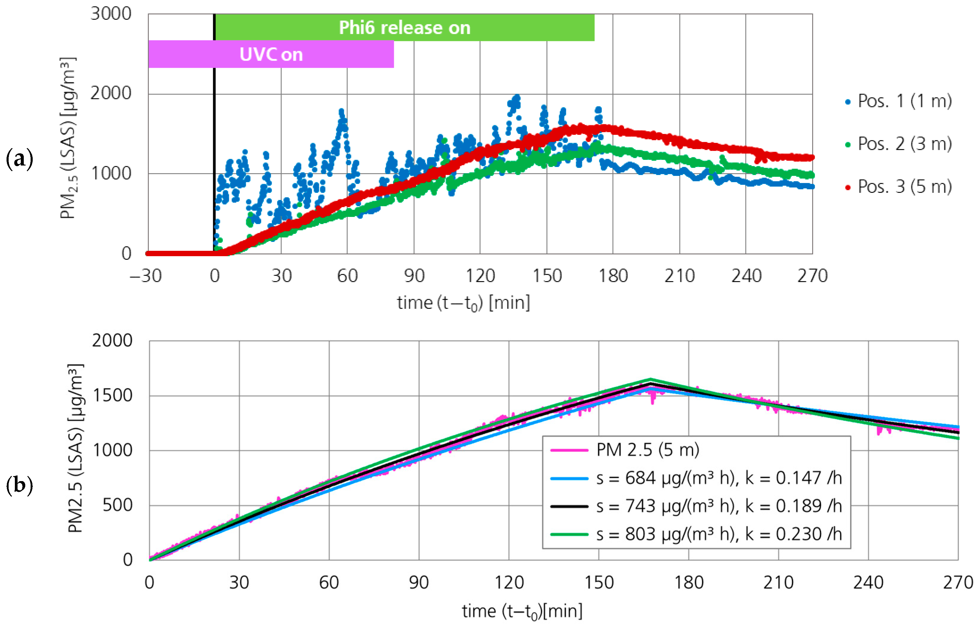
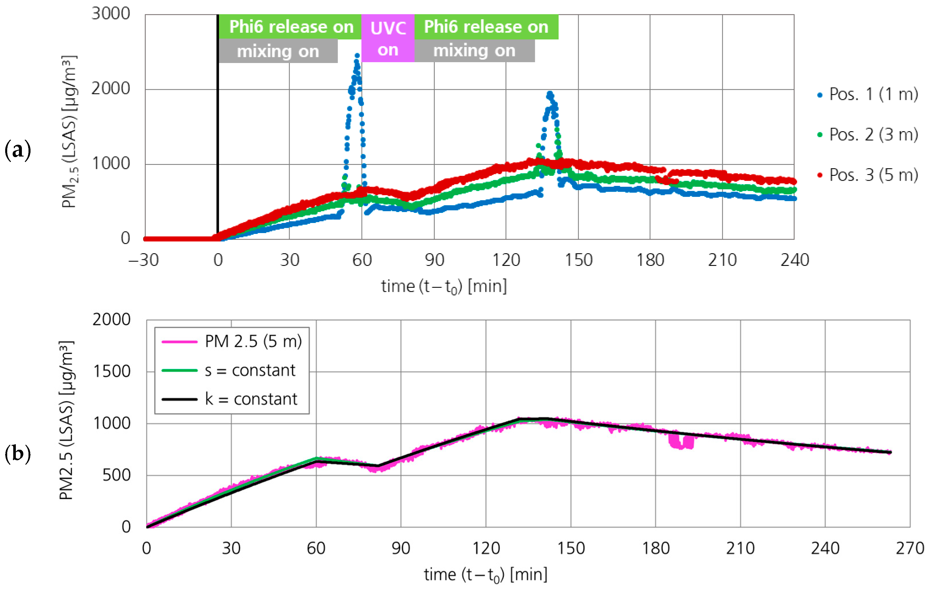
3.1.1. Particle Concentration (PM_2.5)

Figure 5a shows the PM_2.5 concentration at three positions in the test room. At the position (Pos.) closest to the source (Pos. 1, blue dots), the measurement signal varied greatly. The concentration profile at the position furthest from the source (Pos. 3, red dots) was relatively uniform. The air sample for the detection of active virus concentration associated with the measurement point at a distance of 5 m from the source (green dot no. 2 in Figure 3) was collected almost at the same position as the particle measurement at Pos. 3 (red dots).

Figure 5b shows that the concentration profile at the position furthest from the source (5 m) barely deviates from the curves calculated by Equations (35) and (38), with t₀ = 0 min, t₁ = 167.2 min, source term s = 743 ± 59 µg/(m³ h), and k = 0.189 ± 0.041 h⁻¹. Therefore, it can be assumed that the source term for PM_2.5 remained constant over time. In combination with the confirmed stable concentration of active Phi6 in the used bacteriophage suspension, the release of aerosolized Phi6 can be considered constant during the measurement, at least between 09:04:00 (start of concentration increase at Pos. 3) and 11:51:12 (adjusted switch-off time t₁ of the source term at Pos. 3; collection of fourth air sample until 11:51).

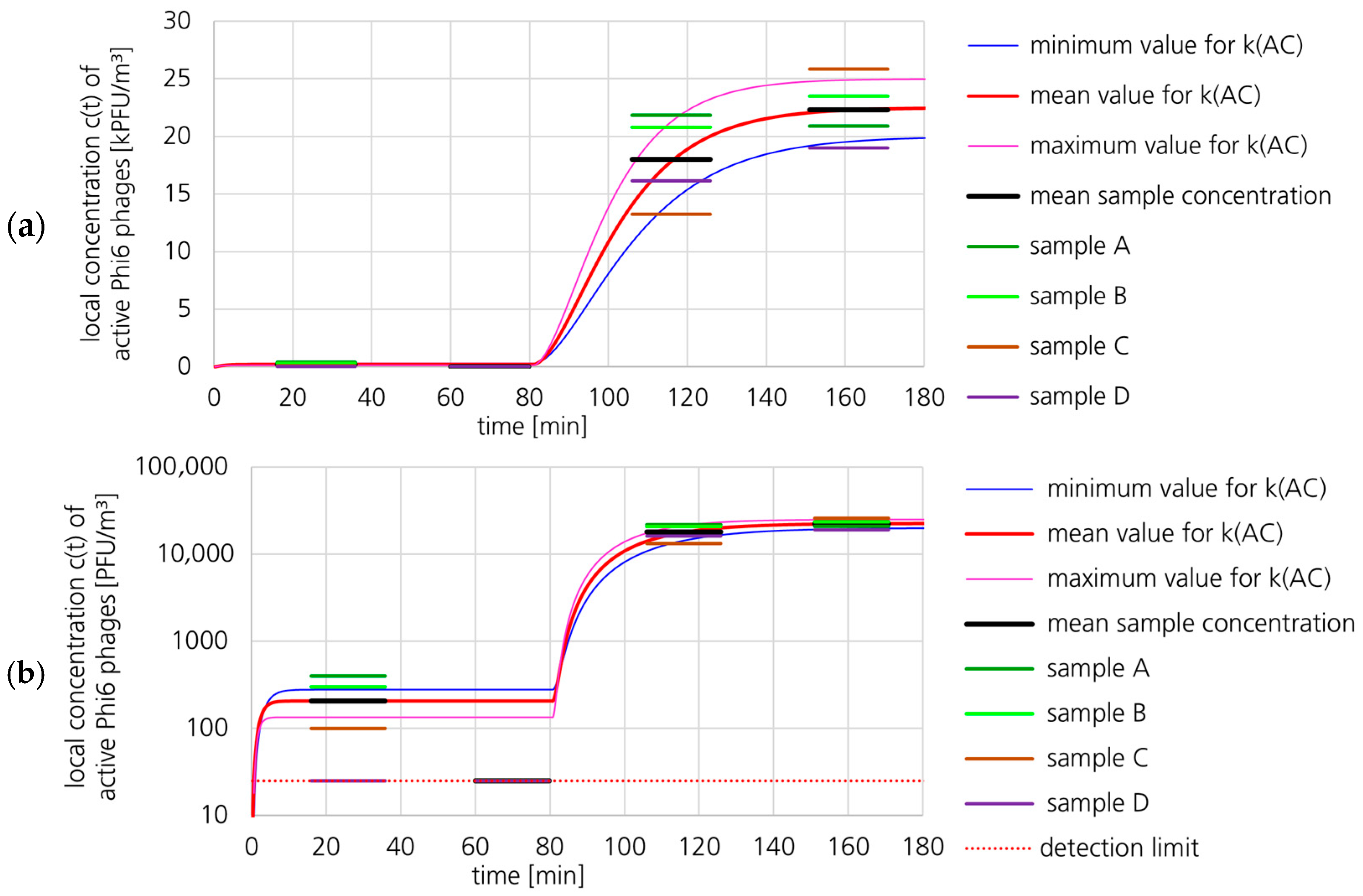
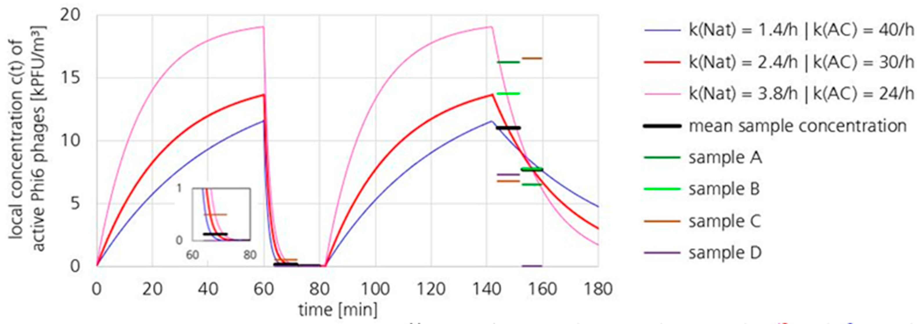
3.1.2. Active Phi6 Concentration at Pos. 2 with Gradient Model and Moderate Uncertainty

Figure 6 shows the mean concentrations of active Phi6 in the indoor air for the plaque assay air samples at Pos. 2 (green dot no. 2 in Figure 3). The concentrations of active Phi6 in the individual samples of the plaque assays are also shown. The concentration of the first two samples varied from the detection limit (25 PFU/m³) up to 400 PFU/m³. The equilibrium concentration c_1eq with UVC switched on (active air cleaner) was 206 PFU/m³ for the 16–36 min sample and below the detection limit for the 60–80 min sample. The concentration of the last sample varied from 19,000 up to 25,850 PFU/m³ (19.00–25.85 kPFU/m³). The calculated concentration profiles linked to minimum and maximum k_AC values are shown for moderate parameter uncertainties. The concentration profiles in Figure 6 were calculated with the gradient model (Equation (24) and equations of Section 2.6.1). The corresponding parameters are listed in

Table 4. Mean values and deviations of the parameters used to calculate the active Phi6 concentration c(t) and the loss coefficient k_AC at Pos. 2 with gradient model and moderate uncertainty.

	Mean Value	Deviation Absolute	Deviation Relative	Partial or Total Uncertainty for kAC [h−1]	Minimum Value	Maximum Value
kNat [h−1]	5.0	0.75	15%	7.1 (1)	4.25	5.75
c1eq [PFU/m3]	206	72	35%	9.1 (1)	134	278
c2eq [PFU/m3]	22,500	2500	11%	2.9 (1)	20,000	25,000
kAC [h−1]	47.3	n.a. (2)	25%	11.9 (3)	32 (4)	73 (5)

(1) partial uncertainty calculated with the corresponding term of Equation (26); (2) not applicable; (3) total uncertainty calculated by Equation (26); (4) calculated by Equation (24) with minimum values of k_Nat and c_2eq and maximum value of c_1eq; (5) calculated by Equation (24) with maximum values of k_Nat and c_2eq and minimum value of c_1eq.

. For the equilibrium concentration c_1eq, the mean concentration of the first sample (16–36 min) was used (206 PFU/m³). Since the concentration of the second sample was below the detection limit and therefore lower, this choice results in an underestimation of the parameter k_AC. When the mean concentration of the first air sample (sample 16–36 min) was used for c_1eq, the loss coefficient k_AC was 47.3 h⁻¹ and the concentration at the sampling position was reduced by the UR-UVGI system by a factor of 109. When the detection limit (sample 60–80 min) was used for c_1eq, the inactivation loss coefficient k_AC was 145 h⁻¹ and the concentration at the sampling position was reduced by a factor of 900. The major challenge in analyzing data from such highly effective inactivation systems is to measure the Phi6 concentration while the system is active.

The parameters (including their uncertainties or deviations) used to adjust the concentration profiles to the sample concentrations determined by plaque assays are summarized in Table 4. The loss coefficient k_AC was calculated by Equation (24). The uncertainty Δk_AC was calculated by Equation (26). For the equilibrium concentration c_1eq and the absolute deviation of this value, the plaque assay samples from 16 to 36 min were used. The parameters k_Nat and c_2eq were adjusted to match the mean concentrations in the samples from 106 to 126 min and 151 to 171 min. For the absolute deviation of the parameter c_2eq, the plaque assay results of the last sample were used. The deviation of the natural loss coefficient k_Nat was selected by varying this parameter and selecting an appropriate value.

The resulting uncertainty of the parameter k_AC was 25%, or k_AC = 47.3 ± 11.9 h⁻¹ (minimum: 35.3 h⁻¹, maximum: 59.2 h⁻¹). In addition to the calculation using Equation (26), the minimum and maximum values of k_AC were also calculated directly using the minimum and maximum parameter values from Table 4 (minimum k_AC: 32 h⁻¹, maximum k_AC: 73 h⁻¹). Both calculation methods yielded similar results.

With the parameter values of Table 4, the uncertainty of parameter c_1eq contributes 59% to the uncertainty of the result for k_AC. The contribution of k_Nat is 35%, while that of c_2eq is just 6%. Since the concentration in the second air sample (sample 60–80 min) was below the detection limit and the first air sample (sample 16–36 min) was used for this calculation, the contribution of the uncertainty of the parameter c_1eq to the uncertainty of k_AC is by far the largest.

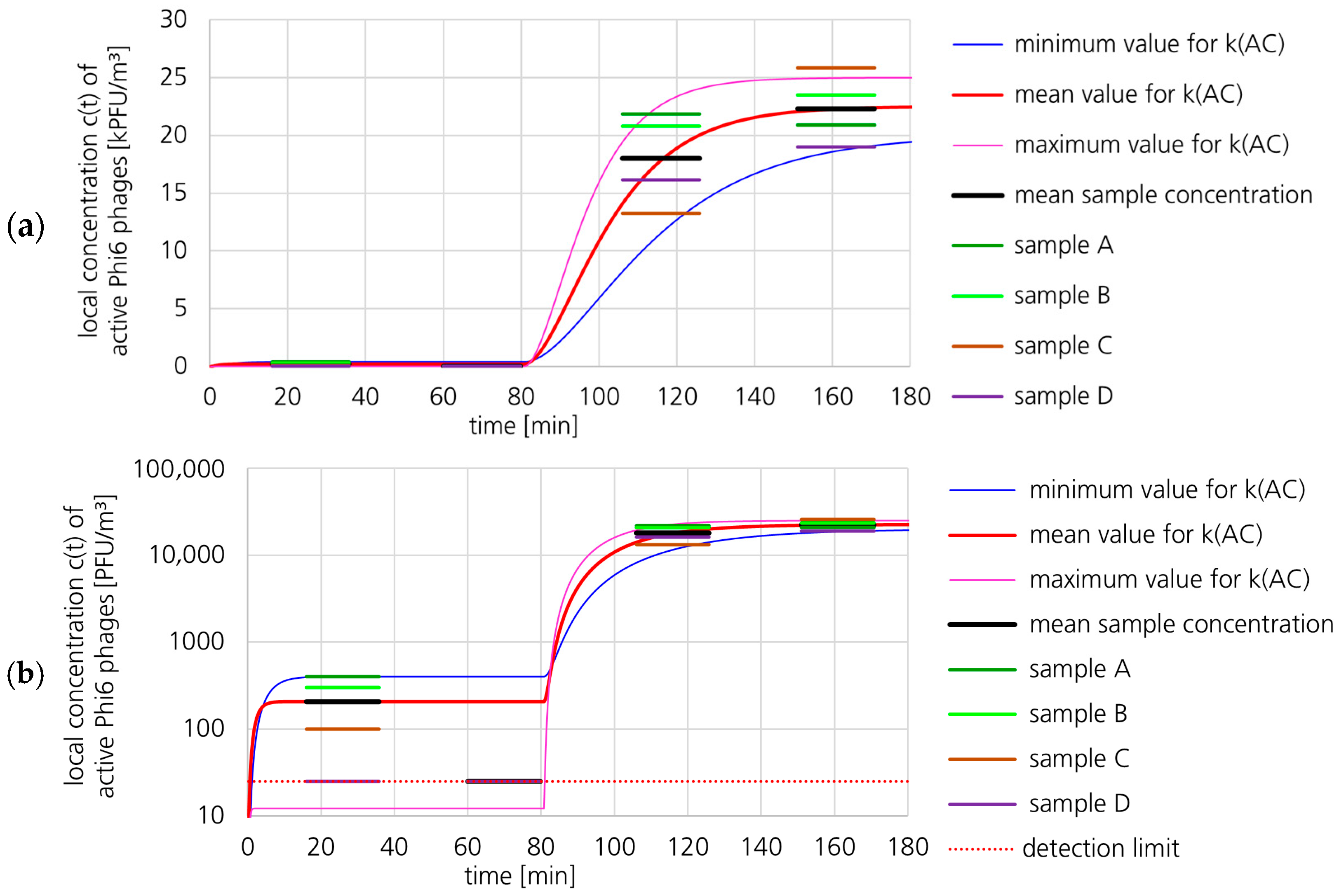
3.1.3. Active Phi6 Concentration at Pos. 2 with Gradient Model and High Uncertainty

Figure 7 shows the same concentrations of active Phi6 in the indoor air for the plaque assay air samples at Pos. 2 (green dot no. 2 in Figure 3) as Figure 6. Except for the parameter uncertainty values, the same values as in Section 3.1.2 were used. The concentration profiles in Figure 7 were calculated with the equations of Section 2.6.1 (gradient model). The calculated concentration profiles linked to minimum and maximum k_AC values are shown for high parameter uncertainties.

The parameters (including their uncertainties or deviations) used for the concentration profiles in Figure 7 are summarized in

Table 5. Mean values and deviations of the parameters used to calculate the active Phi6 concentration c(t) and the loss coefficient k_AC at Pos. 2 with gradient model and high uncertainty.

	Mean Value	Deviation Absolute	Deviation Relative	Partial or Total Uncertainty for kAC [h−1]	Minimum Value	Maximum Value
kNat [h−1]	5.0	1.75	35%	16.5 (1)	3.25	6.75
c1eq [PFU/m3]	206	194	94%	24.6 (1)	12	400
c2eq [PFU/m3]	22,500	2500	11%	2.9 (1)	20,000	25,000
kAC [h−1]	47.3	n.a. (2)	63%	29.8 (3)	19.7 (4)	301 (5)

(1) partial uncertainty calculated with the corresponding term of Equation (26); (2) not applicable; (3) total uncertainty calculated by Equation (26); (4) calculated by Equation (24) with minimum values of k_Nat and c_2eq and maximum value of c_1eq; (5) calculated by Equation (24) with maximum values of k_Nat and c_2eq and minimum value of c_1eq.

. The loss coefficient k_AC was calculated by Equation (24). The uncertainty Δk_AC was calculated by Equation (26). The uncertainties of the parameters were increased to high and very conservative values (35%, 94%, 11% deviation) compared to the moderate values listed in Table 4 (15%, 35%, 11% deviation).

The resulting uncertainty of the parameter k_AC was 63%, or k_AC = 47.3 ± 29.8 h⁻¹ (minimum: 17.5 h⁻¹, maximum: 77.0 h⁻¹). In addition to the calculation using Equation (26), the minimum and maximum values of k_AC were also calculated directly using the minimum and maximum parameter values from Table 5 (minimum k_AC: 19.7 h⁻¹, maximum k_AC: 301 h⁻¹). The deviations of these values from those calculated using Equation (26) are due to the fact that Equation (26) extrapolates the slope from the partial derivative (defined as parameter uncertainty).

A comparison of the results calculated with high uncertainties (Table 5) and moderate uncertainties (Table 4) showed that the high uncertainties led to a smaller deviation of the minimum k_AC (19.7 h⁻¹ vs. 32 h⁻¹) than for the maximum k_AC (301 h⁻¹ vs. 73 h⁻¹). Therefore, the value for k_AC is more likely to be underestimated than overestimated.

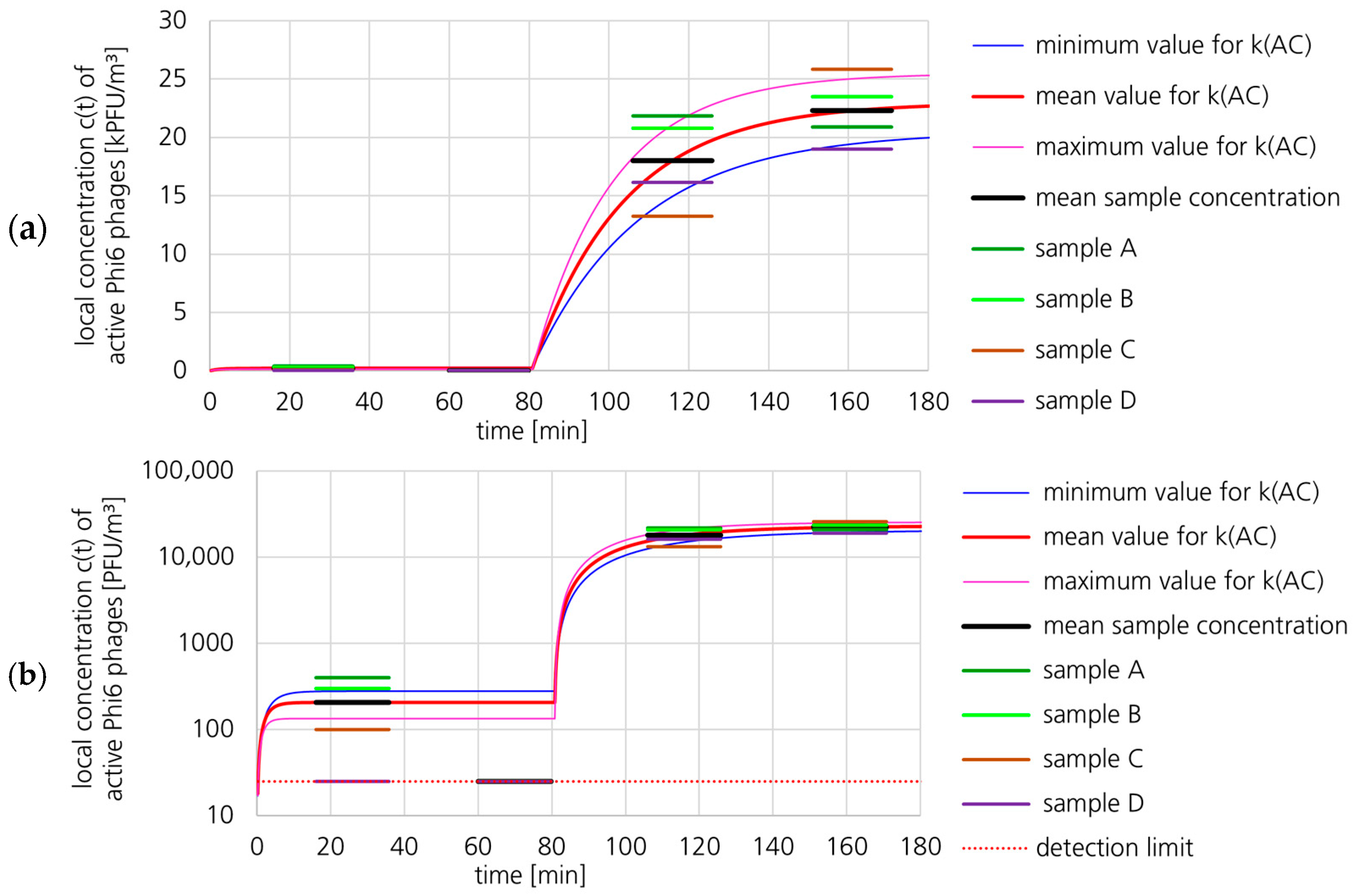
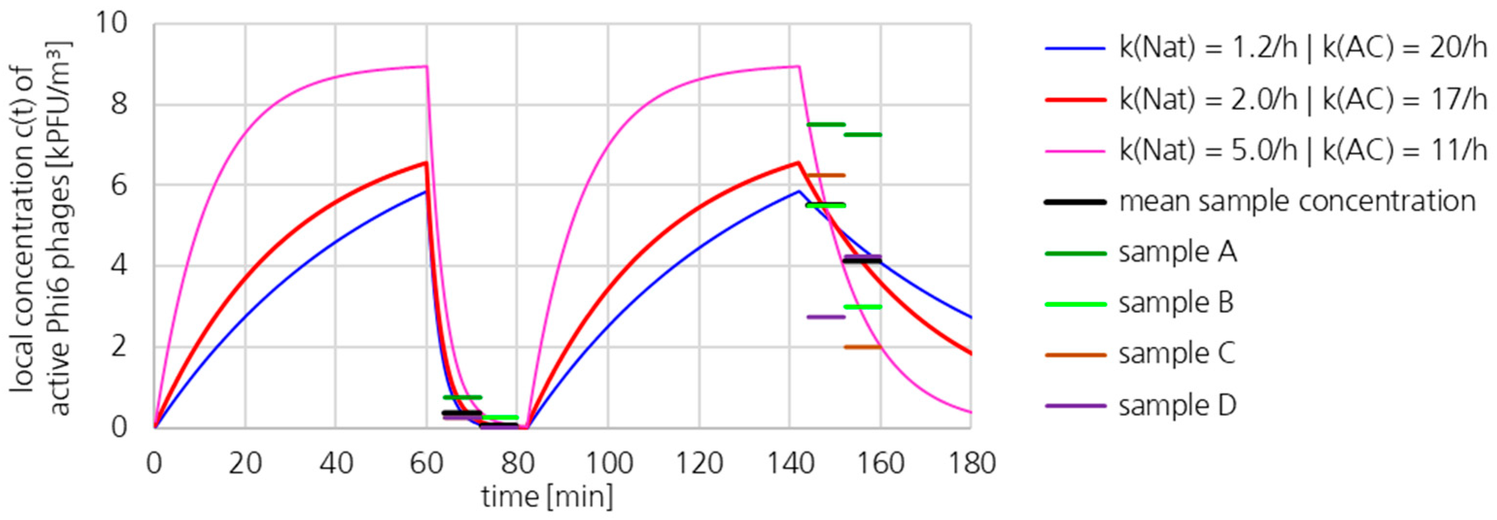
3.1.4. Active Phi6 Concentration at Pos. 2 with Well-Mixed Model and Moderate Uncertainty

Figure 8 shows the same concentrations of active Phi6 in the indoor air for the plaque assay air samples at Pos. 2 (green dot no. 2 in Figure 3) as Figure 6. Except for the calculation model (well-mixed model instead of gradient model), the same values as in Section 3.1.2 were used.

The concentration profiles in Figure 8 were calculated with the equations of Section 2.7.1 (well-mixed model). The calculated concentration profiles linked to minimum and maximum k_AC values are shown for moderate parameter uncertainties.

The parameters (including their uncertainties or deviations) used for the concentration profiles in Figure 8 are summarized in

Table 6. Mean values and deviations of the parameters used to calculate the active Phi6 concentration c(t) and the loss coefficient k_AC at Pos. 2 with the well-mixed model and moderate uncertainty.

	Mean Value	Deviation Absolute	Deviation Relative	Partial or Total Uncertainty for kAC [h−1]	Minimum Value	Maximum Value
kNat [h−1]	2.60	0.39	15%	43 (1)	2.21	2.99
c1eq [PFU/m3]	206	72	35%	102 (1)	134	278
c2eq [PFU/m3]	23,000	2500	11%	32 (1)	20,500	25,500
kAC [h−1]	288	n.a. (2)	40%	115 (3)	161 (4)	566 (5)

(1) partial uncertainty calculated with the corresponding term of Equation (32); (2) not applicable; (3) total uncertainty calculated by Equation (32); (4) calculated by Equation (31) with minimum values of k_Nat and c_2eq and maximum value of c_1eq; (5) calculated by Equation (31) with maximum values of k_Nat and c_2eq and minimum value of c_1eq.

. The loss coefficient k_AC was calculated by Equation (31). The uncertainty Δk_AC was calculated by Equation (32). The uncertainties of the parameters were equal to the values listed in Table 4 (15%, 35%, and 11% deviation).

The resulting uncertainty of the parameter k_AC was 40%, or k_AC = 288 ± 115 h⁻¹ (minimum: 173 h⁻¹, maximum: 403 h⁻¹). In addition to the calculation using Equation (32), the minimum and maximum values of k_AC were also calculated directly using the minimum and maximum parameter values from Table 6 (minimum k_AC: 161 h⁻¹, maximum k_AC: 566 h⁻¹). Both calculation methods yielded similar results.

The evaluation based on the well-mixed model showed that the results for k_AC were significantly higher in this model (161–566 h⁻¹) than in the gradient model (32–73 h⁻¹).

However, when using the well-mixed model (Section 2.7.1) to determine k_Nat in combination with the gradient model (Section 2.6.2) to determine k_AC, the value for k_AC (24.9 h⁻¹) was even lower than when calculated using the gradient model for k_Nat (k_AC = 47.3 h⁻¹), see Table 4 and

Table 7. Mean values and deviations of the parameters used to calculate the active Phi6 concentration c(t) and the loss coefficient k_AC at Pos. 2 with the gradient model and moderate uncertainty.

	Mean Value	Deviation Absolute	Deviation Relative	Partial or Total Uncertainty for kAC [h−1]	Minimum Value	Maximum Value
kNat [h−1]	2.60	0.39	15%	3.7 (1)	2.21	2.99
c1eq [PFU/m3]	206	72	35%	4.8 (1)	134	278
c2eq [PFU/m3]	23,000	2500	11%	1.5 (1)	20,500	25,500
kAC [h−1]	24.9	n.a. (2)	25%	6.3 (3)	17 (4)	38 (5)

(1) partial uncertainty calculated with the corresponding term of Equation (26); (2) not applicable; (3) total uncertainty calculated by Equation (26); (4) calculated by Equation (24) with minimum values of k_Nat and c_2eq and maximum value of c_1eq; (5) calculated by Equation (24) with maximum values of k_Nat and c_2eq and minimum value of c_1eq.

.

Overall, the value of 24.9 h⁻¹ (Table 7) for k_AC is very conservative and tends to be too low and the value of 288 h⁻¹ (Table 6) is unrealistically high.

The resulting uncertainty of the parameter k_AC in Table 7 was 25%, or k_AC = 24.9 ± 6.3 h⁻¹ (minimum: 18.6 h⁻¹, maximum: 31.1 h⁻¹). In addition to the calculation using Equation (26), the minimum and maximum values of k_AC were also calculated directly using the minimum and maximum parameter values from Table 7 (minimum k_AC: 16.8 h⁻¹, maximum k_AC: 38.3 h⁻¹). Both calculation methods yielded similar results.

With the parameter values of Table 7, the uncertainty of parameter c_1eq contributes 59% to the uncertainty of the result for k_AC. The contribution of k_Nat is 35%, while that of c_2eq is just 6%. Since the concentration in the second air sample (sample 60–80 min) was below the detection limit and the first air sample (sample 16–36 min) was used for this calculation, the contribution of the uncertainty of the parameter c_1eq to the uncertainty of k_AC is by far the largest. When the detection limit (25 PFU/m³) would be used for c_1eq, the inactivation Phi6 loss coefficient k_AC would be 76.3 h⁻¹.

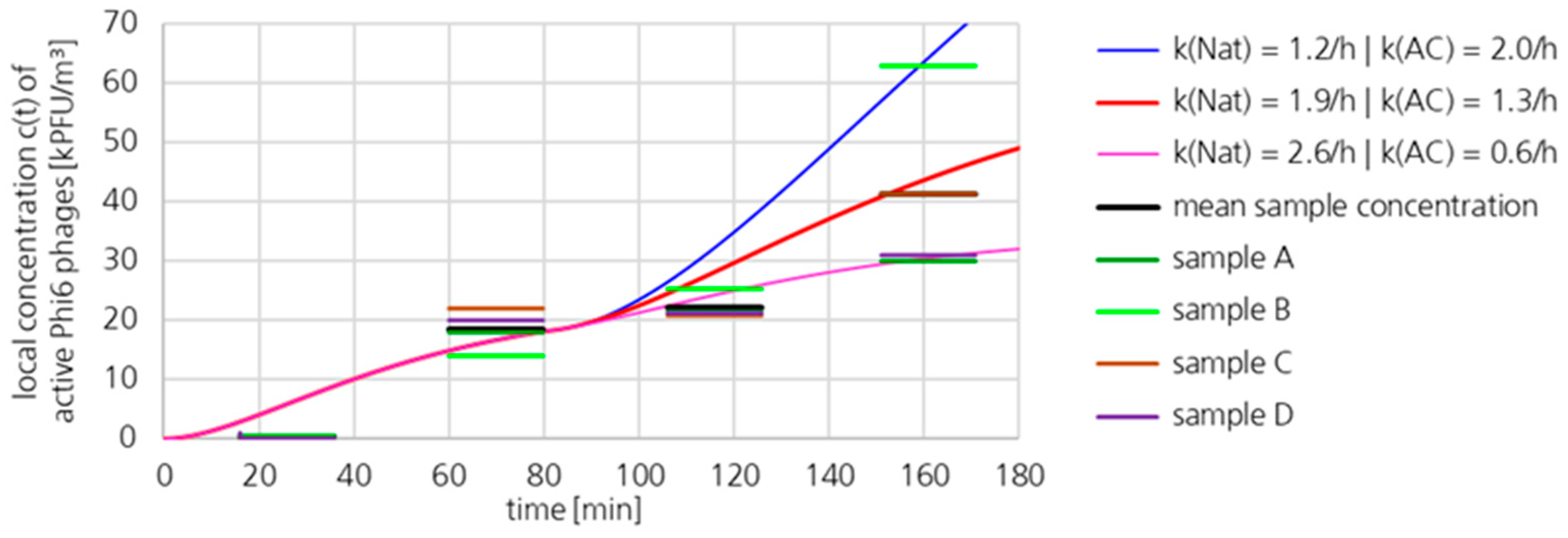
3.1.5. Active Phi6 Concentration at Pos. 1

Figure 9 shows the mean concentrations of active Phi6 in the indoor air at Pos. 1 (green dot no. 1 in Figure 3). The concentrations of active Phi6 in the individual samples of the plaque assays are also shown. The concentration profiles, calculated with the gradient model, are shown for the adjusted parameters c_1eq, c_2eq, and k_Nat for the position in addition to the Sheffield head perpendicular to the breathing direction. The concentration profile at the location near the source is likely to be influenced mainly by changes in the source term. The reason why almost no inactivating effect could be detected at this location is probably a short-circuit air flow directly from the source to the sampling at Pos. 1. The values obtained for the loss coefficient k_AC should be viewed with caution, as it can be assumed that the concentration profile was mainly influenced by changes in the source term. In addition, the plaque assay results were subject to considerable uncertainty.

The important result of the measurement near the source is that no significant inactivation effect could be detected. Considering the extreme effect at the second sampling location (Pos. 2, Section 3.1.2), this result is remarkable. It should be emphasized that measurements without continuous dosing do not capture this effect.

3.2. Loss Coefficient k_AC of the UR-UVGI System Determined by Exponential Decay

3.2.1. Particle Concentration (PM_2.5)

Figure 10a shows the PM_2.5 concentration at three positions in the test room. At the position closest to the source (Pos. 1, blue dots), the measurement signal temporarily increased when the fans mixing the air were turned off 10 min before the aerosol release was stopped. The concentration profile at the position furthest from the source (Pos. 3, red dots) was relatively uniform. The air sampling for the plaque assay test at Pos. 2 (green dot no. 2 in Figure 3) was carried out in close proximity to the particle measurement at Pos. 3 (red dots).

Figure 10b shows the concentration profile at Pos. 3 (5 m) and two calculated concentration profiles. In

Table 8. Fitting parameters k [h⁻¹] and s [µg/(m³ h)] of the two curves in Figure 10b. The blue values were used for adjusting the fit to the measurement data.

Line in Figure 9	Fit Parameter	0–60 min	60–82 min	82–132 min	132–142 min	142–260 min
s = constant	k [h−1]	0.322	0.322	0.322	0.664	0.178
(green line)	s [µg/(m3 h)]	781	0	781	781	0
k = constant	k [h−1]	0.185	0.185	0.185	0.185	0.185
(black line)	s [µg/(m3 h)]	696	0	696	201	0

the adjustment parameters are listed for a fit with a constant loss coefficient k (black line) and for a fit with a constant source term s (green line). When the loss coefficient k is kept constant, the source term s was 696 µg/(m³ h) between 0 and 60 min and between 82 and 132 min, but 201 µg/(m³ h) between 132 and 142 min.

These adjustment parameters indicate that the source term has decreased significantly in the last 10 min before the second exponential decay was measured (determination of k_Nat). Therefore, the assumption of a constant source term throughout the entire experiment may not be accurate.

To test the alternative of a constant source term, the k_Nat values were adjusted separately for each subrange (0–132 min, 132–142 min, 142–260 min), and the source term was kept constant (green line in Figure 10b), values in Table 8). In this case, the loss coefficient would have to increase by 0.342 h⁻¹ at 132 min and decrease by 0.486 h⁻¹ 10 min later.

After 142 min, the source term s is equal to zero and the loss coefficient k is the only fitting parameter. Since the loss coefficient during this period is approximately 0.18 h⁻¹, which is the same value as in the variant with the constant loss coefficient, this variant is more plausible.

Until 132 min, both parameters can be constant over time in both scenarios. Therefore, it can be assumed that the source term for PM_2.5 was constant until 132 min. However, between 132 min and 142 min, the source term dropped significantly. Overall, these results indicate that the Phi6 concentration was higher at 60 min than at 142 min. The smaller peak at 132 min for the concentration at Pos. 1 (blue dots in Figure 10a) compared to the peak at 50 min confirms the hypothesis that the source term was smaller at 132 min than at 50 min. In combination with the confirmed stable concentration of active Phi6 in the used bacteriophage suspension, the release of aerosolized Phi6 can be considered slightly higher for the first (0–60 min) than for the second (82–142 min) Phi6 release. Since the aerosol loss coefficient differs from the Phi6 loss coefficient, no attempt was made to quantify the concentration difference at both positions.

3.2.2. Active Phi6 Concentration at Pos. 2

Figure 11 shows the mean concentrations of active Phi6 in the indoor air at Pos. 2 (green dot no. 2 in Figure 3). The concentrations of active Phi6 in the individual samples of the plaque assays are also shown.

The concentration profiles, calculated with the well-mixed model, are shown for the adjusted parameters c_eq and k_Nat. The loss coefficient k_Nat and the equilibrium concentration c_eq were determined between 144 min and 160 min, and the loss coefficient k_AC between 64 min and 80 min. A constant source term and a constant k_Nat were assumed.

The results from Section 3.2.1 indicate that the concentration at the beginning of the measurement with the active UR-UVGI system (60–82 min) was higher than at the beginning of the natural decay measurement (after 142 min). Therefore, the concentration reduction was underestimated, and thus also the value of k_AC.

3.2.3. Active Phi6 Concentration at Pos. 1

Figure 12 shows the mean concentrations of active Phi6 in the indoor air at Pos. 1 (green dot no. 1 in Figure 3). The concentrations of active Phi6 in the individual samples of the plaque assays are also shown. The concentration profiles, calculated with the well-mixed model, are shown for the adjusted parameters c_eq and k_Nat.

The loss coefficient k_Nat and the equilibrium concentration c_eq were determined between 144 min and 160 min, and the loss coefficient k_AC between 64 min and 80 min. A constant source term and a constant k_Nat were assumed for the calculations.

The results from Section 3.2.1 indicate that the concentration at the beginning of the measurement with the active UR-UVGI system (60–82 min) was higher than at the beginning of the natural decay measurement (after 142 min). Therefore, the concentration reduction was underestimated, and thus also the value of k_AC.

3.3. Summary of Determined Loss Coefficients

In

Table 9. Summary of determined inactivation loss coefficients k_AC and natural loss coefficients k_Nat.

Position in the Test Room	Dynamic Equilibrium			Exponential Decay
(Compare Figure 3)	kAC [h−1]	kNat [h−1]	FR (1)	kAC [h−1]	kNat [h−1]	FR (2)
Pos. 2	47 (32–73) (3) 288 (161–566) (4) 25 (17–38) (5)	5.0 (4.25–5.75) (3) 2.6 (2.21–2.99) (4) 2.6 (2.21–2.99) (5)	109 (3) 111 (4) 111 (5)	30 (24–40)	2.4 (1.4–3.8)	182
Pos. 1	1.3 (0.6–2.0) (6)	1.9 (1.2–2.6) (6)	<2.8 (6)	17 (11–20)	2.0 (1.2–5.0)	90

(1) Reduction factor F_R = c_eq2/c_eq1 (measured values used). (2) Reduction factor F_R = (k_AC/k_Nat + 1)² (calculated for gradient conditions). (3) Utilization of the gradient model for k_Nat and Equation (24) for k_AC. (4) Utilization of the well-mixed model for k_Nat and Equation (31) for k_AC. (5) Utilization of the well-mixed model for k_Nat and Equation (24) for k_AC. (6) Evaluation model was not suitable. It can be assumed that the concentration profile was mainly influenced by changes in the source term.

the determined Phi6 loss coefficients are summarized. The fitted natural loss coefficients were between 1.2 and 5.75 h⁻¹ and hence higher than typical natural loss coefficients for aerosols or particles (0.1–1.5 h⁻¹). The reason for this is that the effects caused by biological inactivation are added to the effects that occur with aerosols.

When the well-mixed model was used for the determination of the natural Phi6 loss coefficient k_Nat at Pos. 2, the value in the dynamic equilibrium measurement (2.6 h⁻¹) was similar to that in the exponential decay measurement (2.4 h⁻¹). In combination with the gradient model for the determination of k_AC, these results were similar for both measurements as well (30 h⁻¹ vs. 25 h⁻¹). On the one hand, this indicates that without an inactivating system, mixing occurs rapidly enough to allow the well-mixed model to be applied. On the other hand, if the UR-UVGI system is active, the gradient model must be used to determine k_AC, as the well-mixed model would result in unrealistically high values for k_AC (288 h⁻¹).

The log reduction for an exponential decline within 10 min and within half an hour corresponding to the determined loss coefficients is listed in

Table 10. Summary of determined loss coefficients and corresponding log reduction values for 10 min and 30 min active UR-UVGI system.

Parameter	Natural Loss (Without UVC)	UVC Loss Pos. 2 Exponential Decline	UVC loss Pos. 2 (1) Dynamic Equilibrium	UVC Loss Pos. 2 (2) Dynamic Equilibrium
Loss coefficient k [h−1]	2.8 (1.2–5.75)	30 (24–40)	47 (32–73)	25 (17–38)
Log reduction in 10 min [-]	0.2 (0.1–0.4)	2.2 (1.7–2.9)	3.4 (2.3–5.3)	1.8 (1.2–2.8)
Log reduction in 30 min [-]	0.6 (0.3–1.2)	6.5 (5.2–8.7)	10.2 (6.9–15.9)	5.4 (3.7–8.3)

(1) Utilization of the gradient model for k_Nat and Equation (24) for k_AC. (2) Utilization of the well-mixed model for k_Nat and Equation (24) for k_AC.

.

4. Discussion

4.1. Fundamental Considerations

The loss coefficient should be high enough to significantly reduce the probability of infection by an infectious person in the room (=continuous source). Assuming a natural loss coefficient of 3 h⁻¹ and a purifier loss coefficient of 12 h⁻¹, the concentration is decreased by factors of 4.5 or 1800, respectively, half an hour after the infected person has left the room. At first glance, it appears that the air purifier has a significant impact on the (biologically active) virus concentration, reducing it by a factor of 400 in just half an hour. However, if the infected person remains in the room, with the same parameters and under well-mixed conditions, the concentration is only reduced by a factor of 5 (=12/3 + 1) by the air purifier. It should be considered that, regarding the risk of infection, this reduction of the virus concentration by the air purifier could easily be overcompensated by the reverse effect of low humidity. Low humidity has two main effects: some microorganisms remain biologically active for a longer time (higher number of active viruses inhaled), and the barrier function of the respiratory tract can be less effective (higher probability of infecting the host).

If the source of the virus is unknown, the options for reducing the virus concentration near the source are limited. Due to this lack of knowledge, the measures must be implemented preventively. This in turn means that high security requirements must be met and that the measures must be as inconspicuous as possible. For example, FFP2 masks or other personalized solutions may be effective but are rarely accepted as a preventive measure. Inactivation of microorganisms can be achieved throughout the entire room by releasing reactive compounds (radicals, ions, ozone) or by irradiating the entire room with germicidal radiation. In practice, completely illuminating an entire room quickly reaches its limits. Both approaches must be critically examined in terms of potential health risks to people in the room.

4.2. Interpretation of the Test Results

Based on the measured flow velocities, the following assumption regarding the theoretically maximum achievable virtual air exchange rate can be determined under the selected test conditions. Assuming a vertical flow velocity between 0.04 m/s and 0.15 m/s and a cycle path length between 6 m and 4 m, a theoretical air exchange rate between 24 h⁻¹ (0.04 m/s and 6 m) and 135 h⁻¹ (0.15 m/s and 4 m) can be estimated. The loss coefficients summarized in Section 3.3, between 17 h⁻¹ and 73 h⁻¹ (5 m distance to the source), are in good agreement with these theoretically estimated values. This correlation means that a large percentage of the viruses were already inactivated by a double passage (up and down) through the radiation carpet.

Using the data from Parry-Nweye et al. [47], the natural loss coefficient for Phi6 in air can be calculated for 25% RH and 45% RH. The natural Phi6 loss coefficient determined from this data was approximately 1.0 h⁻¹ for 25% RH and 2.5 h⁻¹ for 45% RH. During the presented measurements, the relative humidity was 32% for the exponential decay measurement and 39% for the dynamic equilibrium measurement. The results for k_Nat listed in Table 9 ranged between 1.2 and 5.75 h⁻¹, with average values between 1.9 and 5.0 h⁻¹, meaning that the values are approximately twice as high as those reported by Parry-Nweye et al. Whether this deviation is significant or not in view of the high determination uncertainty cannot yet be assessed due to the small amount of data available.

The natural loss coefficients determined using the well-mixed model (2.2–3.0 h⁻¹) tend to be closer to the values calculated using the data from Parry-Nweye et al. (1.0–2.5 h⁻¹) than those determined using the gradient model (4.2–5.8 h⁻¹). In addition, the well-mixed model produces a result (2.6 h⁻¹) that is more similar to the results of the exponential decay measurements (2.4 h⁻¹ or 2.0 h⁻¹). This indicates that the well-mixed model is more suitable for determining k_Nat than the gradient model.

The age of the aerosol may have an influence on the (experimental) natural Phi6 loss coefficient. The continuous release also allows phages that are unstable in the air and become inactive after a short time to be detected. If, on the other hand, the influx of freshly aerosolized phages is eliminated, the (experimental) natural Phi6 loss coefficient could be lower, as the unstable phages have already been excluded from detection. Therefore, a slightly higher k_Nat value for the measurement with continuous Phi6 release could be plausible.

In contrast to the determination of k_Nat, the determination of k_AC using the gradient model provides more plausible results. It is important to note that under well-mixed conditions the measured concentration ratios c_2eq/c_1eq between 109 and 900 in combination with k_Nat = 2 h⁻¹ would correspond to inactivation loss coefficients between 216 h⁻¹ and 1798 h⁻¹. This would result in non-realistic vertical flow velocities up to 3 m/s (1798 h⁻¹ and 6 m cycle length). In addition, the gradient model produces a result (25 h⁻¹) that is more similar to the results of the exponential decay measurements (30 h⁻¹ or 17 h⁻¹). This indicates that the gradient model is more suitable for determining k_AC than the well-mixed model.

Therefore, the combination of the well-mixed model for determining k_Nat with the gradient model for determining k_AC is preferable. This approach results in 25 h⁻¹ for k_AC and 2.6 h⁻¹ for k_Nat.

Riley et al. used the bacterium Serratia marcescens to investigate the influence of convection and air mixing on the inactivating efficiency of upper air disinfection systems [16,45]. They reported virtual air exchange rates (=loss coefficients) of up to 300 air changes (AC) per hour (=300 h⁻¹) [45]. However, during the measurement, there was an additional air exchange that forced the flow through the irradiated zone. Furthermore, no direct comparison is possible because the microorganisms used differ greatly from one another. However, this result shows that very high loss coefficients are achievable.

The results of Section 3.1.5 show that although the UR-UVGI system was active, almost no inactivation effect was observed at the position 1 m away from the Phi6 source. In this case, the concentration profile was probably influenced mainly by changes in the source term. This could be explained by short-circuit airflows directly from the Phi6 source to the sample location without passing through the radiation carpet. One advantage of test procedures in which microorganisms or particles are continuously released is that such local short-circuit airflows can be detected.

The results of the measurement near the source provide an indication of how relevant the local flow conditions might be. Horizontal air currents can result in contaminated air flowing less frequently through the UVC radiation carpet before reaching another person. Horizontal currents can be caused by walking people or by air flowing from one room opening to another.

The major challenge in analyzing measurement data with highly effective inactivating systems is measuring the concentration of biologically active microorganisms while the system is active. An exponential decay with a total loss coefficient of 32 h⁻¹ results in a reduction by a factor of 1 million within 26 min. Therefore, test procedures for air purifiers that use the concentration decline (release off) instead of the dynamic equilibrium (release on) rely on rapid sampling methods and, due to the low sample volumes, microbiological analysis methods with high sensitivity. This means that for measurements with a continuous source, other methods can be used that would not be suitable for measuring an exponential decline.

Furthermore, test procedures without continuous release do not cover the spatio-temporal behavior. The cleaning effect of “whole room solutions” like the upper-room UVC systems should and can be divided into the spatio-temporal source term effect and the effect due to the loss coefficient of the inactivating system itself (Section 2.6.2). The lower influx of active microorganisms from the immediate vicinity means a lower local source term. Therefore, the concentration is reduced both by a lower source term and by a higher concentration loss due to the local inactivation of microorganisms. This means that when estimating the concentration reduction by a “whole room system”, the ratio of the estimated total loss coefficients with and without an inactivating system is squared in the calculation (Equation (24)). This is relevant, for example, if the loss coefficient is derived from vertical flow velocities or virtual air exchange rates, respectively. Furthermore, the source term effect and thus the change in the calculation of the inactivation effect must be considered when comparing upper-room UVC systems with filtering systems.

In a previous publication, six air-cleaning devices with different inactivating units based on plasma or UVC technology were examined. The investigations were carried out under permanent virus release into the room throughout the entire test period to elucidate the realistic efficiency of constant virus emission by a person [80].

Measurements with continuous release of microorganisms in a dynamic equilibrium have proven reliable. Overall, the test procedure (dynamic equilibrium vs. exponential decay) was less susceptible to handling errors, and the test conditions were more stable, particularly regarding the aerosolization of microorganisms.

One limitation of the presented investigations is that both measurements (dynamic equilibrium and exponential decay) were only performed once, meaning that no conclusions can be drawn about reproducibility and only limited conclusions can be drawn about measurement uncertainty. Therefore, further investigations are necessary to evaluate both the test procedure (including the test evaluation) and the inactivation system under investigation.

4.3. Results Regarded as By-Products

During the measurements, there was an increase in ozone concentration regardless of the switching times of the UVC radiation. According to VDI-EE 4300 Sheet 14 [63], the tolerable residual ozone concentration that can be additionally emitted into indoor spaces by the air purifier is 5 ppb or 10 µg/m³. This requirement for tolerable residual ozone concentration was met by the UR-UVGI system.

Ozone is not produced by UV radiation with a wavelength above 250 nm [54]. The formation of ozone can be prevented by filtering out wavelengths below 250 nm (e.g., by using a special glass instead of quartz glass for mercury lamps) or by using radiation sources that do not emit radiation below 250 nm (e.g., UV-LEDs, for example, with a peak wavelength of 260 or 280 nm).

During operation of the UR-UVGI system, only a slight increase in the total concentration of volatile organic compounds (TVOC) was detected (+59 µg/m³ non-separable and identifiable hydrocarbons C9 to C13). With a TVOC background of around 1000 µg/m³, the increase was approximately 6%. This is within the measurement uncertainty. The UV-absorbing film, which was attached to the walls to protect people against scattered radiation, is suspected to be the source of the TVOC background and the increase in TVOC emissions during UVC irradiation.

4.4. UVC LED Technoloqy and Energy Concerns

The entire UR-UVGI system used in the test room required 216 W (measured value). Based on the room size of 129 m³ and the determined loss coefficient (virus inactivation by the purification system) of 25 h⁻¹ (at least 17 h⁻¹ and up to 73 h⁻¹), a clean air delivery rate (CADR) of approximately 3200 m³/h was achieved. To achieve a comparable CADR with filtering air purification systems, a power output of roughly 150 to 500 W would be required. The sound pressure level of such systems is usually around 60 dB(A). UR-UVGI systems, on the other hand, operate almost silently.

As long as the entire light emitted by a low-pressure mercury vapor lamp can be used (for example, in ventilation ducts), these radiation sources are very efficient. However, directed beams are required to form a radiation carpet. This requirement creates advantages for UVC LED technology.

The current development of UVC LEDs is progressing rapidly [20,21,22,56,81,82,83,84,85]. Increases in efficiency can currently be observed with LEDs with a wavelength of 265 nm [56].

4.5. UVC LED Technoloqy and Safety Concerns

UVC radiation is known to pose health risks to humans, including corneal irritation, conjunctival irritation, skin irritation, and skin cancer [6,7,86]. Görlitz et al. have discussed safety aspects for far-UVC technologies [87]. Far-UVC (wavelength < 240 nm) is less hazardous to humans [6] but has the disadvantage of producing undesirable by-products [55].

Hence, upper room disinfection systems are not without controversy due to the UVC radiation used in the room. The planning and installation of the devices should be carried out by specialists. The operation of upper room systems can be safe if all regulations for the manufacture, installation, and operation of the devices are complied with. However, the greatest source of uncertainty in practice is human beings. Brickner and Vincent discussed safety-related aspects using a historical example and showed that, despite a safety concept, people were unintentionally exposed to UVC radiation in practice [88]. Depending on their design, upper room disinfection systems in Europe are covered by the Machinery Directive (2006/42/EC) [89] or the Low Voltage Directive (2014/35/EU) [90]. In both cases, a risk assessment must be carried out in accordance with DIN EN ISO 12100 [91]. DIN EN ISO 60335-2-65 [92] was used for the UVC-specific regulations on electrical safety. The photobiological safety, which is regulated in the European Union’s directive on artificial optical radiation (2006/25/EU) [93], is more complex. In DIN EN 62471 [94], UVC products are categorized into risk groups in accordance with DIN EN IEC 62471-6 [95]. The used UR-UVGI system belongs to risk group 3. Products in risk group 3 must be labelled with the corresponding warnings “UVC” and “do not look directly into the source”. In addition, there must be a switch-off component that recognizes persons or objects in the radiation field. As a protective component, the used UR-UVGI system has a lidar sensor that detects objects in the beam path and switches the system off immediately if necessary.

With the used UR-UVGI system, a separate risk assessment will be carried out before each installation, depending on the room conditions and usage. The EU directive for artificial optical radiation [93] specifies a maximum spectral daily value of 30 J/m². UVC radiation is invisible to the human eye, which is why it must be ensured that people are not accidentally exposed to it. It is important to distinguish between a configuration in which UVC radiation is emitted into the area where people are present or, as in UR-UVGI systems, directly below the ceiling and thus above the typical area where people are present. The difference is crucial for the specifications of the safety components that ensure that the UVC radiation is switched off when necessary.

When calculating the minimum height for the used UR-UVGI system, the divergence of the UVC radiation must be considered. Furthermore, scattered radiation from walls or other surfaces must be considered due to the far-reaching UVC radiation. If necessary, absorbent materials must be attached to the walls.

4.6. Transfer of the Test Results to Other Interiors and Environmental Conditions

Harmon et al. presented in 2022 the Facility Infection Risk Estimator^TM [96]. The probability of infection calculations used by this model are based on a modified version of the Wells–Riley model of infection and include a loss coefficient for the inactivation effect of upper-room UVGI systems. However, they also pointed out that the various indoor influences on the inactivation efficiency of UR-UVGI systems cannot be adequately taken into account in the model, as the interactions are not yet fully understood.

The results of the investigations are strongly influenced by the interior conditions. Thermal convection and thus the vertical mixing of the indoor air depend in particular on the number of people or thermal manikins (hot zones) and the temperatures of the wall or window surfaces (cold zones). For this reason, computer models are needed to simulate the results and transfer them to other indoor conditions. Examples of such computer models are the zonal models of Matheis et al. [97] or Leithäuser et al. [98], the multi-zonal model of Nicas and Miller [99], and the CFD model of Noakes et al. [23].

5. Conclusions

Apart from measurements in flow channels and small flow chambers, there are hardly any studies in which microorganisms are continuously released into the air during the actual measurement. Combining this with purification systems that inactivate airborne microorganisms across the entire ceiling surface further reduces the number of relevant studies. In addition, information is often missing that would allow data to be converted into loss coefficients. This makes comparison with other studies difficult.

The results presented show that measurements with continuous release of microorganisms and comparison of the dynamic equilibrium with and without inactivation technology have several advantages over measurements of exponential decay curves and that they can be evaluated by the mathematical model described in this publication.

Test procedures for systems in which the air to be cleaned is passed through a device are not particularly suitable for inactivating systems that use the entire room area or even the entire room volume for inactivation. One reason for this is that such “whole-room systems” use thermal convection in the room, circulation systems that operate independently of the inactivating system, or act directly in the entire room, so that no defined volume flow can be assigned to the tested system. Therefore, the tests should be carried out under test conditions that are as realistic and at the same time as reproducible as possible. The results of the measurements near the source provide an indication of how relevant the local flow conditions might be. Advances in computer simulations ultimately help to transfer the data obtained to other interior and flow conditions.

For “whole-room systems”, the ratio F_R of the steady-state concentrations without and with the inactivating system can be expressed as a product of a factor F_k due to a loss coefficient effect and a factor F_s due to a source term effect. In general, this product can be described as F_R = F_k × F_s = F_R^a × F_R^1−a. In this publication, the value 0.5 was selected for variable a. This means that both factors influence the result in equal measure. If the variable a is not equal to 0.5, this changes the formula used to calculate k_AC. Further investigations are needed to determine whether the assumption a = 0.5 accurately describes the experimental behavior or whether adjustments are necessary.

Furthermore, the test procedure should be investigated regarding repeatability, reproducibility, and reliability. In addition, the parameters that most strongly influence UR-UVGI inactivation effectiveness should be investigated in order to avoid failure of the inactivation effect in real-life situations.

The inactivation of pathogenic microorganisms in indoor spaces using UVC radiation is not a new technology. In fact, UVC radiation has been used for almost a century to reduce the transmission of diseases [88,100]. However, advances in UVC LED technology [56,81,84] and LED optics [76,101] in recent years, combined with efforts to replace mercury-based technologies (254 nm) [102,103] and findings that excimer lamps (222 nm) produce undesirable by-products [55], have created a new situation.

Overall, the results demonstrate that UR-UVGI systems can inactivate the surrogate virus Phi6 very effectively under realistic testing conditions, with loss coefficients (or virtual air exchange rates) of approximately 25 h⁻¹, at least above 17 h⁻¹. Miller wrote back in 2015 [26]: “Why this technology has yet to be widely implemented, as an engineering control strategy to combat airborne disease transmission, is somewhat of a mystery”.

6. Patents

The used optical arrangement is a system patented (WO2021249668A1) by the company Smart United GmbH [76].

References

1. Gomes, M.; Bartolomeu, M.; Vieira, C.; Gomes, A.T.P.C.; Faustino, M.A.F.; Neves, M.G.P.M.S.; Almeida, A. Photoinactivation of Phage Phi6 as a SARS-CoV-2 Model in Wastewater: Evidence of Efficacy and Safety. Microorganisms 2022, 10, 659. [Google Scholar] [CrossRef]
2. Bartolomeu, M.; Braz, M.; Costa, P.; Duarte, J.; Pereira, C.; Almeida, A. Evaluation of UV-C Radiation Efficiency in the Decontamination of Inanimate Surfaces and Personal Protective Equipment Contaminated with Phage ϕ6. Microorganisms 2022, 10, 593. [Google Scholar] [CrossRef] [PubMed]
3. Gidari, A.; Sabbatini, S.; Bastianelli, S.; Pierucci, S.; Busti, C.; Bartolini, D.; Stabile, A.M.; Monari, C.; Galli, F.; Rende, M.; et al. SARS-CoV-2 Survival on Surfaces and the Effect of UV-C Light. Viruses 2021, 13, 408. [Google Scholar] [CrossRef]
4. Belland, K.; Garcia, D.; DeJohn, C.; Allen, G.R.; Mills, W.D.; Glaudel, S.P. Safety and Effectiveness Assessment of Ultraviolet-C Disinfection in Aircraft Cabins. Aerosp. Med. Hum. Perform. 2024, 95, 147–157. [Google Scholar] [CrossRef] [PubMed]
5. Allen, G.R.; Benner, K.J.; Bahnfleth, W.P. Inactivation of Pathogens in Air Using Ultraviolet Direct Irradiation Below Exposure Limits. J. Res. Natl. Inst. Stand. Technol. 2021, 126, 126052. [Google Scholar] [CrossRef]
6. Sliney, D.H.; Stuck, B.E. A Need to Revise Human Exposure Limits for Ultraviolet UV-C Radiation. Photochem. Photobiol. 2021, 97, 485–492. [Google Scholar] [CrossRef]
7. Sliney, D. Balancing the risk of eye irritation from UV-C with infection from bioaerosols. Photochem. Photobiol. 2013, 89, 770–776. [Google Scholar] [CrossRef]
8. Bang, J.-I.; Kim, J.-H.; Choi, A.; Sung, M. The Wavelength-Based Inactivation Effects of a Light-Emitting Diode Module on Indoor Microorganisms. Int. J. Environ. Res. Public Health 2022, 19, 9659. [Google Scholar] [CrossRef]
9. Zhu, S.; Srebric, J.; Rudnick, S.N.; Vincent, R.L.; Nardell, E.A. Numerical investigation of upper-room UVGI disinfection efficacy in an environmental chamber with a ceiling fan. Photochem. Photobiol. 2013, 89, 782–791. [Google Scholar] [CrossRef]
10. Zhu, S.; Lin, T.; Wang, L.; Nardell, E.A.; Vincent, R.L.; Srebric, J. Ceiling impact on air disinfection performance of Upper-Room Germicidal Ultraviolet (UR-GUV). Build. Environ. 2022, 224, 109530. [Google Scholar] [CrossRef]
11. Yıldırım, G.; Kılıç, H.; Karakaş, H.M. The antimicrobial efficacy of shielded ultraviolet germicidal irradiation in CT rooms with intense human circulation. Diagn. Interv. Radiol. 2021, 27, 293–301. [Google Scholar] [CrossRef]
12. Yao, G.; Liu, Z.; Liu, H.; Jiang, C.; Li, Y.; Liu, J.; He, J. Air disinfection performance of upper-room ultraviolet germicidal irradiation (UR-UVGI) system in a multi-compartment dental clinic. J. Hazard. Mater. 2024, 477, 135383. [Google Scholar] [CrossRef]
13. Yang, Y.; Lai, A.C.; Wu, C. Study on the disinfection efficiency of multiple upper-room ultraviolet germicidal fixtures system on airborne microorganisms. Build. Environ. 2016, 103, 99–110. [Google Scholar] [CrossRef]
14. Wang, M.H.; Zhang, H.H.; Chan, C.K.; Lee, P.; Lai, A. Experimental study of the disinfection performance of a 222-nm Far-UVC upper-room system on airborne microorganisms in a full-scale chamber. Build. Environ. 2023, 236, 110260. [Google Scholar] [CrossRef]
15. Shen, J.; Kong, M.; Dong, B.; Birnkrant, M.J.; Zhang, J. Airborne transmission of SARS-CoV-2 in indoor environments: A comprehensive review. Sci. Technol. Built Environ. 2021, 27, 1331–1367. [Google Scholar] [CrossRef]
16. Riley, R.L.; Permutt, S.; Kaufman, J.E. Room air disinfection by ultraviolet irradiation of upper air. Further analysis of convective air exchange. Arch. Environ. Health 1971, 23, 35–39. [Google Scholar] [CrossRef]
17. Riley, R.L.; Permutt, S. Room air disinfection by ultraviolet irradiation of upper air. Air mixing and germicidal effectiveness. Arch. Environ. Health 1971, 22, 208–219. [Google Scholar] [CrossRef]
18. Reed, N.G. The history of ultraviolet germicidal irradiation for air disinfection. Public Health Rep. 2010, 125, 15–27. [Google Scholar] [CrossRef]
19. Park, S.; Mistrick, R.; Rim, D. Performance of upper-room ultraviolet germicidal irradiation (UVGI) system in learning environments: Effects of ventilation rate, UV fluence rate, and UV radiating volume. Sustain. Cities Soc. 2022, 85, 104048. [Google Scholar] [CrossRef]
20. Nunayon, S.S.; Zhang, H.; Lai, A.C.K. Comparison of disinfection performance of UVC-LED and conventional upper-room UVGI systems. Indoor Air 2020, 30, 180–191. [Google Scholar] [CrossRef]
21. Nunayon, S.S.; Zhang, H.H.; Lai, A.C.K. A novel upper-room UVC-LED irradiation system for disinfection of indoor bioaerosols under different operating and airflow conditions. J. Hazard. Mater. 2020, 396, 122715. [Google Scholar] [CrossRef]
22. Nunayon, S.S.; Wang, M.; Zhang, H.H.; Lai, A.C.K. Evaluating the efficacy of a rotating upper-room UVC-LED irradiation device in inactivating aerosolized Escherichia coli under different disinfection ranges, air mixing, and irradiation conditions. J. Hazard. Mater. 2022, 440, 129791. [Google Scholar] [CrossRef]
23. Noakes, C.J.; Beggs, C.B.; Sleigh, P.A. Modelling the Performance of Upper Room Ultraviolet Germicidal Irradiation Devices in Ventilated Rooms: Comparison of Analytical and CFD Methods. Indoor Built Environ. 2004, 13, 477–488. [Google Scholar] [CrossRef]
24. Nardell, E.; Vincent, R.; Sliney, D.H. Upper-room ultraviolet germicidal irradiation (UVGI) for air disinfection: A symposium in print. Photochem. Photobiol. 2013, 89, 764–769. [Google Scholar] [CrossRef] [PubMed]
25. Nardell, E.A. Indoor environmental control of tuberculosis and other airborne infections. Indoor Air 2016, 26, 79–87. [Google Scholar] [CrossRef]
26. Miller, S.L. Upper Room Germicidal Ultraviolet Systems for Air Disinfection Are Ready for Wide Implementation. Am. J. Respir. Crit. Care Med. 2015, 192, 407–409. [Google Scholar] [CrossRef] [PubMed]
27. Memarzadeh, F.; Olmsted, R.N.; Bartley, J.M. Applications of ultraviolet germicidal irradiation disinfection in health care facilities: Effective adjunct, but not stand-alone technology. Am. J. Infect. Control. 2010, 38, S13–S24. [Google Scholar] [CrossRef]
28. McPhaul, K.M. Indoor Air Disinfection: Answering Questions About Germicidal Ultraviolet Lights. Workplace Health Saf. 2022, 70, 431. [Google Scholar] [CrossRef]
29. McDevitt, J.J.; Milton, D.K.; Rudnick, S.N.; First, M.W. Inactivation of poxviruses by upper-room UVC light in a simulated hospital room environment. PLoS ONE 2008, 3, e3186. [Google Scholar] [CrossRef]
30. Mata, T.M.; Martins, A.A.; Calheiros, C.S.C.; Villanueva, F.; Alonso-Cuevilla, N.P.; Gabriel, M.F.; Silva, G.V. Indoor Air Quality: A Review of Cleaning Technologies. Environments 2022, 9, 118. [Google Scholar] [CrossRef]
31. Liu, C.-Y.; Tseng, C.-H.; Wang, H.-C.; Dai, C.-F.; Shih, Y.-H. The Study of an Ultraviolet Radiation Technique for Removal of the Indoor Air Volatile Organic Compounds and Bioaerosol. Int. J. Environ. Res. Public Health 2019, 16, 2557. [Google Scholar] [CrossRef]
32. Linnes, J.C.; Rudnick, S.N.; Hunt, G.M.; McDevitt, J.J.; Nardell, E.A. Eggcrate UV: A whole ceiling upper-room ultraviolet germicidal irradiation system for air disinfection in occupied rooms. Indoor Air 2014, 24, 116–124. [Google Scholar] [CrossRef]
33. Lee, L.D.; Lie, L.; Bauer, M.; Bolanos, B.; Olmsted, R.N.; Varma, J.K.; Parada, J.P. Reduction of airborne and surface-borne bacteria in a medical center burn intensive care unit using active, upper-room, germicidal ultraviolet (GUV) disinfection. Infect. Control Hosp. Epidemiol. 2024, 45, 367–373. [Google Scholar] [CrossRef]
34. Landry, S.A.; Jamriska, M.; Menon, V.J.; Lee, L.Y.Y.; Magnin-Bougma, I.; Subedi, D.; Barr, J.J.; Monty, J.; Kevin, K.; Gunatilaka, A.; et al. Ultraviolet radiation vs air filtration to mitigate virus laden aerosol in an occupied clinical room. J. Hazard. Mater. 2025, 487, 137211. [Google Scholar] [CrossRef]
35. Kujundzic, E.; Matalkah, F.; Howard, C.J.; Hernandez, M.; Miller, S.L. UV air cleaners and upper-room air ultraviolet germicidal irradiation for controlling airborne bacteria and fungal spores. J. Occup. Environ. Hyg. 2006, 3, 536–546. [Google Scholar] [CrossRef] [PubMed]
36. EPA, U.S.; OAR. What Is Upper-Room Ultraviolet Germicidal Irradiation (UVGI)? What Is HVAC UVGI? Can Either Be Used to Disinfect the Air and Help Protect Myself from COVID? | US EPA. Available online: https://www.epa.gov/indoor-air-quality-iaq/what-upper-room-ultraviolet-germicidal-irradiation-uvgi-what-hvac-uvgi-can (accessed on 1 February 2025).
37. Davidson, B.L. Bare-bulb Upper-Room Germicidal Ultraviolet-C (GUV) Indoor Air Disinfection for COVID-19. Photochem. Photobiol. 2021, 97, 524–526. [Google Scholar] [CrossRef]
38. Challener, D.W.; Tande, A.J.; Koutras, C.; Wade, R.L.; McIntee, M.A.; Strauss, D.M.; Yao, X.; Chang, Y.-H.; Berbari, E. Evaluation of germicidal ultraviolet-C disinfection in a real-world outpatient health care environment. Am. J. Infect. Control 2024, 52, 1030–1034. [Google Scholar] [CrossRef]
39. Bergman, R.S. Germicidal UV Sources and Systems. Photochem. Photobiol. 2021, 97, 466–470. [Google Scholar] [CrossRef]
40. Bergman, R.; Brenner, D.; Buonanno, M.; Eadie, E.; Forbes, P.D.; Jensen, P.; Nardell, E.A.; Sliney, D.; Vincent, R.; Welch, D.; et al. Air Disinfection with Germicidal Ultraviolet: For this Pandemic and the Next. Photochem. Photobiol. 2021, 97, 464–465. [Google Scholar] [CrossRef]
41. Beggs, C.B.; Avital, E.J. Upper-room ultraviolet air disinfection might help to reduce COVID-19 transmission in buildings: A feasibility study. PeerJ 2020, 8, e10196. [Google Scholar] [CrossRef]
42. Bang, J.-I.; Park, J.; Choi, A.; Jeong, J.-W.; Kim, J.Y.; Sung, M. Evaluation of UR-UVGI System for Sterilization Effect on Microorganism Contamination in Negative Pressure Isolation Ward. Sustainability 2018, 10, 3192. [Google Scholar] [CrossRef]
43. Nardell, E.A. Air Disinfection for Airborne Infection Control with a Focus on COVID-19: Why Germicidal UV is Essential. Photochem. Photobiol. 2021, 97, 493–497. [Google Scholar] [CrossRef]
44. Nguyen, T.T.; He, C.; Carter, R.; Ballard, E.L.; Smith, K.; Groth, R.; Jaatinen, E.; Kidd, T.J.; Nguyen, T.-K.; Stockwell, R.E.; et al. The Effectiveness of Ultraviolet-C (UV-C) Irradiation on the Viability of Airborne Pseudomonas aeruginosa. Int. J. Environ. Res. Public Health 2022, 19, 13706. [Google Scholar] [CrossRef]
45. Riley, R.L.; Permutt, S.; Kaufman, J.E. Convection, air mixing, and ultraviolet air disinfection in rooms. Arch. Environ. Health 1971, 22, 200–207. [Google Scholar] [CrossRef]
46. Kheyrandish, A.; Mohseni, M.; Taghipour, F. Protocol for Determining Ultraviolet Light Emitting Diode (UV-LED) Fluence for Microbial Inactivation Studies. Environ. Sci. Technol. 2018, 52, 7390–7398. [Google Scholar] [CrossRef]
47. Parry-Nweye, E.; Liu, Z.; Dhaouadi, Y.; Guo, X.; Huang, W.; Zhang, J.; Ren, D. Persistence of Phi6, a SARS-CoV-2 surrogate, in simulated indoor environments: Effects of humidity and material properties. PLoS ONE 2025, 20, e0313604. [Google Scholar] [CrossRef]
48. French, A.J.; Longest, A.K.; Pan, J.; Vikesland, P.J.; Duggal, N.K.; Marr, L.C.; Lakdawala, S.S. Environmental Stability of Enveloped Viruses Is Impacted by Initial Volume and Evaporation Kinetics of Droplets. mBio 2023, 14, e03452-22. [Google Scholar] [CrossRef]
49. Niazi, S.; Short, K.R.; Groth, R.; Cravigan, L.; Spann, K.; Ristovski, Z.; Johnson, G.R. Humidity-Dependent Survival of an Airborne Influenza A Virus: Practical Implications for Controlling Airborne Viruses. Environ. Sci. Technol. Lett. 2021, 8, 412–418. [Google Scholar] [CrossRef]
50. Prussin, A.J.; Schwake, D.O.; Lin, K.; Gallagher, D.L.; Buttling, L.; Marr, L.C. Survival of the Enveloped Virus Phi6 in Droplets as a Function of Relative Humidity, Absolute Humidity, and Temperature. Appl. Environ. Microbiol. 2018, 84, e00551-18. [Google Scholar] [CrossRef]
51. Plano LMde Franco, D.; Rizzo, M.G.; Zammuto, V.; Gugliandolo, C.; Silipigni, L.; Torrisi, L.; Guglielmino, S.P.P. Role of Phage Capsid in the Resistance to UV-C Radiations. Int. J. Mol. Sci. 2021, 22, 3408. [Google Scholar] [CrossRef]
52. Masjoudi, M.; Mohseni, M.; Bolton, J.R. Sensitivity of Bacteria, Protozoa, Viruses, and Other Microorganisms to Ultraviolet Radiation. J. Res. Natl. Inst. Stand. Technol. 2021, 126, 126021. [Google Scholar] [CrossRef]
53. Oh, C.; Sun, P.P.; Araud, E.; Nguyen, T.H. Mechanism and efficacy of virus inactivation by a microplasma UV lamp generating monochromatic UV irradiation at 222 nm. Water Res. 2020, 186, 116386. [Google Scholar] [CrossRef]
54. Claus, H. Ozone Generation by Ultraviolet Lamps. Photochem. Photobiol. 2021, 97, 471–476. [Google Scholar] [CrossRef]
55. Sørensen, S.B.; Dalby, F.R.; Olsen, S.K.; Kristensen, K. Influence of Germicidal UV (222 nm) Lamps on Ozone, Ultrafine Particles, and Volatile Organic Compounds in Indoor Office Spaces. Environ. Sci. Technol. 2024, 58, 20073–20080. [Google Scholar] [CrossRef]
56. Ishida, K.; Onoda, Y.; Kadomura-Ishikawa, Y.; Nagahashi, M.; Yamashita, M.; Fukushima, S.; Aizawa, T.; Yamauchi, S.; Fujikawa, Y.; Tanaka, T.; et al. Development of a standard evaluation method for microbial UV sensitivity using light-emitting diodes. Heliyon 2024, 10, e27456. [Google Scholar] [CrossRef]
57. Inagaki, H.; Saito, A.; Kaneko, C.; Sugiyama, H.; Okabayashi, T.; Fujimoto, S. Rapid Inactivation of SARS-CoV-2 Variants by Continuous and Intermittent Irradiation with a Deep-Ultraviolet Light-Emitting Diode (DUV-LED) Device. Pathogens 2021, 10, 754. [Google Scholar] [CrossRef]
58. Takamure, K.; Sakamoto, Y.; Iwatani, Y.; Amano, H.; Yagi, T.; Uchiyama, T. Characteristics of collection and inactivation of virus in air flowing inside a winding conduit equipped with 280 nm deep UV-LEDs. Environ. Int. 2022, 170, 107580. [Google Scholar] [CrossRef]
59. Takamure, K.; Iwatani, Y.; Amano, H.; Yagi, T.; Uchiyama, T. Inactivation characteristics of a 280 nm Deep-UV irradiation dose on aerosolized SARS-CoV-2. Environ. Int. 2023, 177, 108022. [Google Scholar] [CrossRef]
60. Karimzadeh, S.; Bhopal, R.; Nguyen Tien, H. Review of infective dose, routes of transmission and outcome of COVID-19 caused by the SARS-COV-2: Comparison with other respiratory viruses. Epidemiol. Infect. 2021, 149, e96. [Google Scholar] [CrossRef]
61. Turgeon, N.; Toulouse, M.-J.; Martel, B.; Moineau, S.; Duchaine, C. Comparison of five bacteriophages as models for viral aerosol studies. Appl. Environ. Microbiol. 2014, 80, 4242–4250. [Google Scholar] [CrossRef]
62. Sankaran, A.; Hain, R.; Matheis, C.; Fuchs, T.; Norrefeldt, V.; Grün, G.; Kähler, C.J. Investigation on the thermal budget and flow field of a manikin and comparison with human subject in different scenarios. Build. Environ. 2024, 252, 111290. [Google Scholar] [CrossRef]
63. VDI-EE 4300-Blatt 14; Messen Von Innenraumluftverunreinigungen—Anforderungen an Mobile luftreiniger Zur Reduktion der Aerosolgebundenen Übertragung Von Infektionskrankheiten. Measurement of Indoor Pollution—Requirements for Mobile Air Purifiers to Reduce Aerosol-Borne Transmission of Infectious Diseases. VDI: Düsseldorf, Germany, 2021.
64. ANSI/AHAM AC-1-2020; Method for Measuring Performance of Portable Household Electric Room Air Cleaners. American National Standards Institute and White Goods Manufacturers Association: Washington, DC, USA, 2020.
65. de Aquino Carvalho, N.; Stachler, E.N.; Cimabue, N.; Bibby, K. Evaluation of Phi6 Persistence and Suitability as an Enveloped Virus Surrogate. Environ. Sci. Technol. 2017, 51, 8692–8700. [Google Scholar] [CrossRef]
66. Whitworth, C.; Mu, Y.; Houston, H.; Martinez-Smith, M.; Noble-Wang, J.; Coulliette-Salmond, A.; Rose, L. Persistence of Bacteriophage Phi 6 on Porous and Nonporous Surfaces and the Potential for Its Use as an Ebola Virus or Coronavirus Surrogate. Appl. Environ. Microbiol. 2020, 86, e01482-20. [Google Scholar] [CrossRef]
67. Weyersberg, L.; Klemens, E.; Buehler, J.; Vatter, P.; Hessling, M. UVC, UVB and UVA susceptibility of Phi6 and its suitability as a SARS-CoV-2 surrogate. AIMS Microbiol. 2022, 8, 278–291. [Google Scholar] [CrossRef]
68. Greenwald, R.; Hayat, M.J.; Dons, E.; Giles, L.; Villar, R.; Jakovljevic, D.G.; Good, N. Estimating minute ventilation and air pollution inhaled dose using heart rate, breath frequency, age, sex and forced vital capacity: A pooled-data analysis. PLoS ONE 2019, 14, e0218673. [Google Scholar] [CrossRef]
69. AHAM AC-5-2022; Method for Assessing the Reduction Rate of Key Bioaero-Sols by Portable Air Cleaners Using an Aerobiology Test Chamber. American National Standards Institute and White Goods Manufacturers Association: Washington, DC, USA, 2022.
70. DIN ISO 16000-16:2009-12; Innenraumluftverunreinigungen-Teil_16: Nachweis Und Zählung Von Schimmelpilzen—Probenahme Durch Filtration (ISO_16000-16:2008). DIN Media GmbH: Berlin, Germany, 2009.
71. DIN ISO 16000-17:2010-06; Innenraumluftverunreinigungen-Teil_17: Nachweis Und Zählung Von Schimmelpilzen—Kultivierungsverfahren (ISO_16000-17:2008). DIN Media GmbH: Berlin, Germany, 2010.
72. Baer, A.; Kehn-Hall, K. Viral concentration determination through plaque assays: Using traditional and novel overlay systems. J. Vis. Exp. JoVE 2014, 93, e52065. [Google Scholar] [CrossRef]
73. DIN EN 13610:2003-06; Chemische Desinfektionsmittel—Quantitativer Suspensionsversuch zur Bestimmung der Viruziden Wirkung gegenüber Bakteriophagen von Chemischen Desinfektionsmitteln in den Bereichen Lebensmittel und Industrie - Prüfverfahren und Anforderungen (Phase 2, Stufe 1). DIN Media GmbH: Berlin, Germany, 2003. [CrossRef]
74. DIN ISO 16000-6:2012-11; Innenraumluftverunreinigungen—Teil 6: Bestimmung von VOC in der Innenraumluft und in Prüfkammern, Probenahme auf Tenax TA®, thermische Desorption und Gaschromatographie mit MS oder MS-FID (ISO_16000-6:2011). Beuth Verlag GmbH: Berlin, Germany, 2012. [CrossRef]
75. DIN ISO 16000-3:2013-01; Innenraumluftverunreinigungen—Teil 3: Messen von Formaldehyd und anderen Carbonylverbindungen in der Innenraumluft und in Prüfkammern—Probenahme mit einer Pumpe (ISO 16000-3:2011). Beuth Verlag GmbH: Berlin, Germany, 2013. [CrossRef]
76. Prohaska, R.; Wieser, A.; Muschaweck, J. Lamp and System with Wall-Type Radiation Fields for Preventing or Minimising the Spread of Pathogens in Indoor Air. WO/2021/249668, 16.12.2021. US20230218791A1, 13 July 2023. [Google Scholar]
77. Schmohl, A.; Buschhaus, M.; Norrefeldt, V.; Johann, S.; Burdack-Freitag, A.; Scherer, C.R.; Vega Garcia, P.A.; Schwitalla, C. Incremental Evaluation Model for the Analysis of Indoor Air Measurements. Atmosphere 2022, 13, 1655. [Google Scholar] [CrossRef]
78. Schumacher, S.; Asbach, C.; Schmid, H.-J. Effektivität von Luftreinigern zur Reduzierung des COVID-19-Infektionsrisikos/Efficacy of air purifiers in reducing the risk of COVID-19 infections. Gefahrstoffe 2021, 81, 16–28. [Google Scholar] [CrossRef]
79. Eadie, E.; Hiwar, W.; Fletcher, L.; Tidswell, E.; O’Mahoney, P.; Buonanno, M.; Welch, D.; Adamson, C.S.; Brenner, D.J.; Noakes, C.; et al. Far-UVC (222 nm) efficiently inactivates an airborne pathogen in a room-sized chamber. Sci. Rep. 2022, 12, 4373. [Google Scholar] [CrossRef]
80. Burdack-Freitag, A.; Buschhaus, M.; Grün, G.; Hofbauer, W.K.; Johann, S.; Nagele-Renzl, A.M.; Schmohl, A.; Scherer, C.R. Particulate Matter versus Airborne Viruses—Distinctive Differences between Filtering and Inactivating Air Cleaning Technologies. Atmosphere 2022, 13, 1575. [Google Scholar] [CrossRef]
81. Chiappa, F.; Frascella, B.; Vigezzi, G.P.; Moro, M.; Diamanti, L.; Gentile, L.; Lago, P.; Clementi, N.; Signorelli, C.; Mancini, N.; et al. The efficacy of ultraviolet light-emitting technology against coronaviruses: A systematic review. J. Hosp. Infect. 2021, 114, 63–78. [Google Scholar] [CrossRef]
82. Dziubenko, O.; Arhun, S.; Hnatov, A.; Bogdan, D.; Patlins, A. Device for Inactivation of SARS-CoV-2 Using UVC LEDs. Elektron. Elektrotechnika 2022, 28, 55–61. [Google Scholar] [CrossRef]
83. Gerchman, Y.; Mamane, H.; Friedman, N.; Mandelboim, M. UV-LED disinfection of Coronavirus: Wavelength effect. J. Photochem. Photobiol. B Biol. 2020, 212, 112044. [Google Scholar] [CrossRef]
84. Hsu, T.-C.; Teng, Y.-T.; Yeh, Y.-W.; Fan, X.; Chu, K.-H.; Lin, S.-H.; Yeh, K.-K.; Lee, P.-T.; Lin, Y.; Chen, Z.; et al. Perspectives on UVC LED: Its Progress and Application. Photonics 2021, 8, 196. [Google Scholar] [CrossRef]
85. Kapse, S.; Rahman, D.; Avital, E.J.; Venkatesan, N.; Smith, T.; Cantero-Garcia, L.; Motallebi, F.; Samad, A.; Beggs, C.B. Conceptual Design of a UVC-LED Air Purifier to Reduce Airborne Pathogen Transmission—A Feasibility Study. Fluids 2023, 8, 111. [Google Scholar] [CrossRef]
86. Ploydaeng, M.; Rajatanavin, N.; Rattanakaemakorn, P. UV-C light: A powerful technique for inactivating microorganisms and the related side effects to the skin. Photodermatol. Photoimmunol. Photomed. 2021, 37, 12–19. [Google Scholar] [CrossRef]
87. Görlitz, M.; Justen, L.; Rochette, P.J.; Buonanno, M.; Welch, D.; Kleiman, N.J.; Eadie, E.; Kaidzu, S.; Bradshaw, W.J.; Javorsky, E.; et al. Assessing the safety of new germicidal far-UVC technologies. Photochem. Photobiol. 2024, 100, 501–520. [Google Scholar] [CrossRef]
88. Brickner, P.W.; Vincent, R.L. Ultraviolet germicidal irradiation safety concerns: A lesson from the Tuberculosis Ultraviolet Shelter Study: Murphy’s Law affirmed. Photochem. Photobiol. 2013, 89, 819–821. [Google Scholar] [CrossRef]
89. European Council. DIRECTIVE 2006/42/EC on Machinery Lays Down Health and Safety Requirements for the Design and Construction of Machinery, Placed on the European Market. Available online: https://eur-lex.europa.eu/eli/dir/2006/42/oj/eng (accessed on 3 July 2025).
90. European Council. DIRECTIVE 2014/35/EU on the Harmonisation of the Laws of the Member States Relating to the Making Available on the Market of Electrical Equipment Designed for Use Within Certain Voltage Limits. 2014. Available online: https://eur-lex.europa.eu/eli/dir/2014/35/oj/eng (accessed on 3 July 2025).
91. DIN EN ISO 12100:2011-03; Sicherheit Von Maschinen—Allgemeine Gestaltungsleitsätze—Risikobeurteilung und Risikominderung (ISO 12100:2010); Deutsche Fassung EN ISO 12100:2010. DIN Media GmbH: Berlin, Germany, 2011.
92. DIN EN 60335-2-65:2013-02; Household and Similar Electrical Appliances—Safety—Part 2–65: Particular Requirements for Air-Cleaning Appliances. DIN Media GmbH: Berlin, Germany, 2013.
93. European Council. DIRECTIVE 2006/25/EC on the Minimum Health and Safety Requirements Regarding the Exposure of Workers to Risks Arising from Physical Agents (Artificial Optical Radiation). 2024. Available online: https://eur-lex.europa.eu/eli/dir/2006/25/oj/eng (accessed on 3 July 2025).
94. DIN EN 62471:2009-03; Photobiological Safety of Lamps and Lamp Systems. DIN Media GmbH: Berlin, Germany, 2009.
95. DIN EN IEC 62471-6:2024-05; Photobiological Safety of Lamps and Lamp Systems—Part 6: Ultraviolet Lamp Products. DIN Media GmbH: Berlin, Germany, 2024.
96. Harmon, M.; Lau, J. The Facility Infection Risk Estimator™: A web application tool for comparing indoor risk mitigation strategies by estimating airborne transmission risk. Indoor Built Environ. 2022, 31, 1339–1362. [Google Scholar] [CrossRef]
97. Matheis, C.; Norrefeldt, V.; Will, H.; Herrmann, T.; Noethlichs, B.; Eckhardt, M.; Stiebritz, A.; Jansson, M.; Schön, M. Modeling the Airborne Transmission of SARS-CoV-2 in Public Transport. Atmosphere 2022, 13, 389. [Google Scholar] [CrossRef]
98. Leithäuser, C.; Norrefeldt, V.; Thiel, E.; Buschhaus, M.; Kuhnert, J.; Suchde, P. Predicting aerosol transmission in airplanes: Benefits of a joint approach using experiments and simulation. Numer. Methods Fluids 2024, 96, 991–1010. [Google Scholar] [CrossRef]
99. Nicas, M.; Miller, S.L. A multi-zone model evaluation of the efficacy of upper-room air ultraviolet germicidal irradiation. Appl. Occup. Environ. Hyg. 1999, 14, 317–328. [Google Scholar] [CrossRef] [PubMed]
100. Riley, R.L.; Nardell, E.A. Clearing the air. The theory and application of ultraviolet air disinfection. Am. Rev. Respir. Dis. 1989, 139, 1286–1294. [Google Scholar] [CrossRef]
101. Chen, Y.; Vallance, R.; Hii, K.-F.; Gordon, P.; Zong, Y.; Miller, C. Stamped metallic optical reflectors for ultraviolet light emitting diodes. In Light-Emitting Devices, Materials, and Applications XXVI; Proceedings SPIE 12022; SPIE: San Francisco, CA, USA, 2022; 120220N (3 March 2022); pp. 1–12. [Google Scholar] [CrossRef]
102. European Council. DIRECTIVE 2011/65/EU on the Restriction of the Use of Certain Hazardous Substances in Electrical and Electronic Equipment. 2011. Available online: https://eur-lex.europa.eu/eli/dir/2011/65/oj/eng (accessed on 3 July 2025).
103. European Union. REGULATION (EU) 2017/852 on Mercury, and Repealing Regulation (EC) No 1102/2008. 2017. Available online: https://eur-lex.europa.eu/eli/reg/2017/852/oj/eng (accessed on 3 July 2025).
Figure 1. IATC test set-up south-facing with the upper-room UVC irradiation system below the ceilling, thermal manikins sitting on chairs and a table in the centre of the “meeting room”: (a) photo; (b) thermal image (blue = minimal temperature, yellow = maximum temperature).
Environments 12 00233 g001
Figure 2. Wall on the eastside of the IATC facility with cooled “window” segments: (a) photo facing southeast; (b) thermal image facing northeast (blue = minimal temperature, yellow = maximum temperature).
Environments 12 00233 g002
Figure 3. Setup in the test room with breathing head as Phi6 source (orange arrow), two sample collection positions for plaque assay air samples (green dots), three particle measurement positions (blue dots), the position of by-product measurements (ozone analyzer, photoionization detector, and volatile organic compound air sample collection; yellow dot), and cold surfaces simulating windows. The used UV-C LED array (purple bar) is described in Section 2.3.
Environments 12 00233 g003
Figure 4. Wavelength emission spectrum of the used UVC LED (NCSU434C, Nichia, Japan).
Environments 12 00233 g004
Figure 5. PM2.5 concentration profile. (a) At three positions in the room during the measurement with continuous Phi6 release. (b) Fit to PM2.5 at position 3 (5 m) with aerosol source off at t1 = 167.2 min, source term s = 743 ± 59 µg/(m3 h), and loss coefficient k = 0.189 ± 0.041 h−1. The black line refers to the optimal fit (three fitting parameters: t1, s, k). The source term was increased by 8% for the green line and decreased by 8% for the blue line (one fitting parameter: k). An uncertainty of 8% in the source term leads to an uncertainty of 22% in the loss coefficient.
Environments 12 00233 g005
Figure 6. Concentration profile and sample concentrations of active Phi6 at Pos. 2 (green dot no. 2 in Figure 3). For the calculation of the concentration profiles, the parameters of Table 4 (moderate uncertainty) and the gradient model were used. (a) Linear y-axis, (b) logarithmic y-axis.
Environments 12 00233 g006
Figure 7. Concentration profile and sample concentrations of active Phi6 at Pos. 2 (green dot no. 2 in Figure 3). For the calculation of the concentration profiles, the parameters of Table 5 (high uncertainty) and the gradient model were used. (a) Linear y-axis, (b) logarithmic y-axis.
Environments 12 00233 g007
Figure 8. Concentration profile and sample concentrations of active Phi6 at Pos. 2 (green dot no. 2 in Figure 3). For the calculation of the concentration profiles, the parameters of Table 6 (moderate uncertainty) and the well-mixed model were used. (a) Linear y-axis, (b) logarithmic y-axis.
Environments 12 00233 g008
Figure 9. Concentration profile and sample concentrations of active Phi6 at Pos. 1 (green dot no. 1 in Figure 3).
Environments 12 00233 g009
Figure 10. PM2.5 profile. (a) At three positions in the room during the measurement with continuous Phi6 release. (b) Fitted profiles to PM2.5 at position 3 (5 m). Fit with k = variable (green) and with k = constant. Parameter values are listed in Table 8.
Environments 12 00233 g010
Figure 11. Concentration profile and sample concentrations of active Phi6 at Pos. 2 (green dot no. 2 in Figure 3). The local UR-UVGI loss coefficient was between 24 and 40 h−1, and the natural loss coefficient was between 1.4 and 3.8 h−1.
Environments 12 00233 g011
Figure 12. Concentration profile and sample concentrations of active Phi6 at Pos 1 (green dot no. 1 in Figure 3). The local UR-UVGI loss coefficient was between 11 and 20 h−1, and the natural loss coefficient was between 1.2 and 5.0 h−1.
Environments 12 00233 g012