An Evaluation of the Influence of Meteorological Factors and a Pollutant Emission Inventory on PM_2.5 Prediction in the Beijing–Tianjin–Hebei Region Based on a Deep Learning Method

Abstract

In this study, a Long Short-Term Memory (LSTM) network approach is employed to evaluate the prediction performance of PM_2.5 in the Beijing–Tianjin–Hebei region (BTH). The proposed method is evaluated using the hourly air quality datasets from the China National Environmental Monitoring Center, European Center for Medium-range Weather Forecasts ERA5 (ECMWF-ERA5), and Multi-resolution Emission Inventory for China (MEIC) for the years 2016 and 2017. The predicted PM_2.5 concentrations demonstrate a strong correlation with the observed values (R² = 0.871–0.940) in the air quality dataset. Furthermore, the model exhibited the best performance in situations of heavy pollution (PM_2.5 > 150 μg/m³) and during the winter season, with respective R² values of 0.689 and 0.915. In addition, the influence of ECMWF-ERA5’s hourly meteorological factors was assessed, and the results revealed regional heterogeneity on a large scale. Further evaluation was conducted by analyzing the chemical components of the MEIC inventory on the prediction performance. We concluded that the same temporal profile may not be suitable for addressing emission inventories in a large area with a deep learning method.

1. Introduction

In recent years, rapid industrialization, urbanization, and economic development have significantly increased anthropogenic air pollutant emissions [1,2] in China. The unfavorable weather conditions [3], coupled with these factors, have led to a severe air pollution problem in the country. In all air pollution events occurring in China over the past decade, the PM_2.5 concentration consistently held the highest ranking within the Individual Air Quality Index (IAQI) among the six categories of pollutants [4]. This elevation in PM_2.5 levels has the potential to exert adverse impacts on atmospheric visibility [5], climate change [6,7], and human health [8,9,10,11,12]. In order to mitigate the detrimental impact, the Chinese government has made extensive efforts to decrease pollutant emissions [13,14,15], with the specific goal of reducing the annual PM_2.5 concentrations nationwide. Particularly, significant measures have been implemented in the Beijing–Tianjin–Hebei region (BTH), Yangtze River Delta region (YRD), and Pearl River Delta region (PRD), leading to noteworthy accomplishments. Nonetheless, intermittent occurrences of haze events still take place in certain instances [16,17]. Hence, the accurate and timely forecasting of PM_2.5 concentrations is imperative for regions that are impacted by PM_2.5 pollution.

There are two primary approaches to air quality forecasting: knowledge-driven models and data-driven models. Knowledge-driven models rely on complex equations that encompass various atmospheric dynamics. These models, such as CMAQ and WRF-Chem [18,19], require high-performance computers but offer limited accuracy. On the other hand, data-driven models have gained significant attention in recent years, particularly with the advent of the third wave of artificial intelligence (AI). Many researchers have successfully employed statistical models, including tree-based models and machine learning algorithms, to predict air quality and achieve satisfactory results. In a recent study, a group of researchers from Taiwan utilized Continuous Emission Monitoring Systems (CEMSs) to enhance prediction accuracy [20]. Their findings demonstrated that incorporating additional features did indeed improve the prediction performance. However, it is important to note that the experiment did not account for the impact of heavily polluted regions. Therefore, in complex air pollutant areas, it is crucial to consider more relevant data to ensure comprehensive analysis and prediction.

The advancement of new information technology, including the Internet of Things (IoT) and AI [21,22,23], has enabled the acquisition and utilization of large-scale data for prompt air quality trend prediction. Meteorological and emission factors are pivotal in the discussion of air pollution causation [24,25,26]. For this study, the European Centre for Medium-range Weather Forecasts ERA5 (ECMWF-ERA5) was selected due to its widespread accessibility and rich repository of meteorological factors, which have demonstrated effective performance in the context of the Chinese Mainland environment [27,28]. In the realm of emission pollutants, a considerable number of researchers have employed the Multi-resolution Emission Inventory for China (MEIC) to obtain high-resolution emission [29] maps for regional air quality predictions. During the data extraction and conversion process, meteorological factors were extracted, and the Sparse Matrix Operator Kernel Emissions Model (SMOKE) [30] was utilized to allocate the raw MEIC data to finely grained temporal and spatial resolutions. Numerous researchers have attested to the robustness of AI in predicting future air quality [31,32,33,34], particularly through the Long Short-Term Memory network (LSTM) deep learning model, which demonstrates proficient performance [35,36,37] in air quality forecasting. To further leverage the potential of the information contained within these accessible data sources, experiments were designed to assess the applicability of the air quality dataset, ECMWF-ERA5 factors, and MEIC emission inventory in the hourly prediction of PM_2.5 concentrations using the LSTM model.

This study developed a PM_2.5 prediction system by extracting air monitoring datasets, ECMWF-ERA5 datasets, and MEIC emission inventory datasets for the target region. By utilizing the LSTM deep learning model and extracted features, the proposed method successfully predicted next-hour PM_2.5 concentrations at 13 individual air monitoring stations in the BTH region for 2016 and 2017.

To the best of our knowledge, this research represents an attempt to develop a PM_2.5 prediction system that evaluates air monitoring datasets, meteorological fields, and local emission inventories in the BTH region. The study involved the following steps: First, the ECMWF-ERA5 and MEIC datasets were tested using the Mann–Kendall test to select the appropriate variables. Secondly, a single LSTM method was introduced to evaluate its superiority in air quality prediction. Thirdly, based on the LSTM method, the performance of the two aforementioned datasets were tested, and it was found that the meteorological dataset exhibited spatial heterogeneity, while the pollutant emission data displayed temporal disparity.

2. Materials and Methods

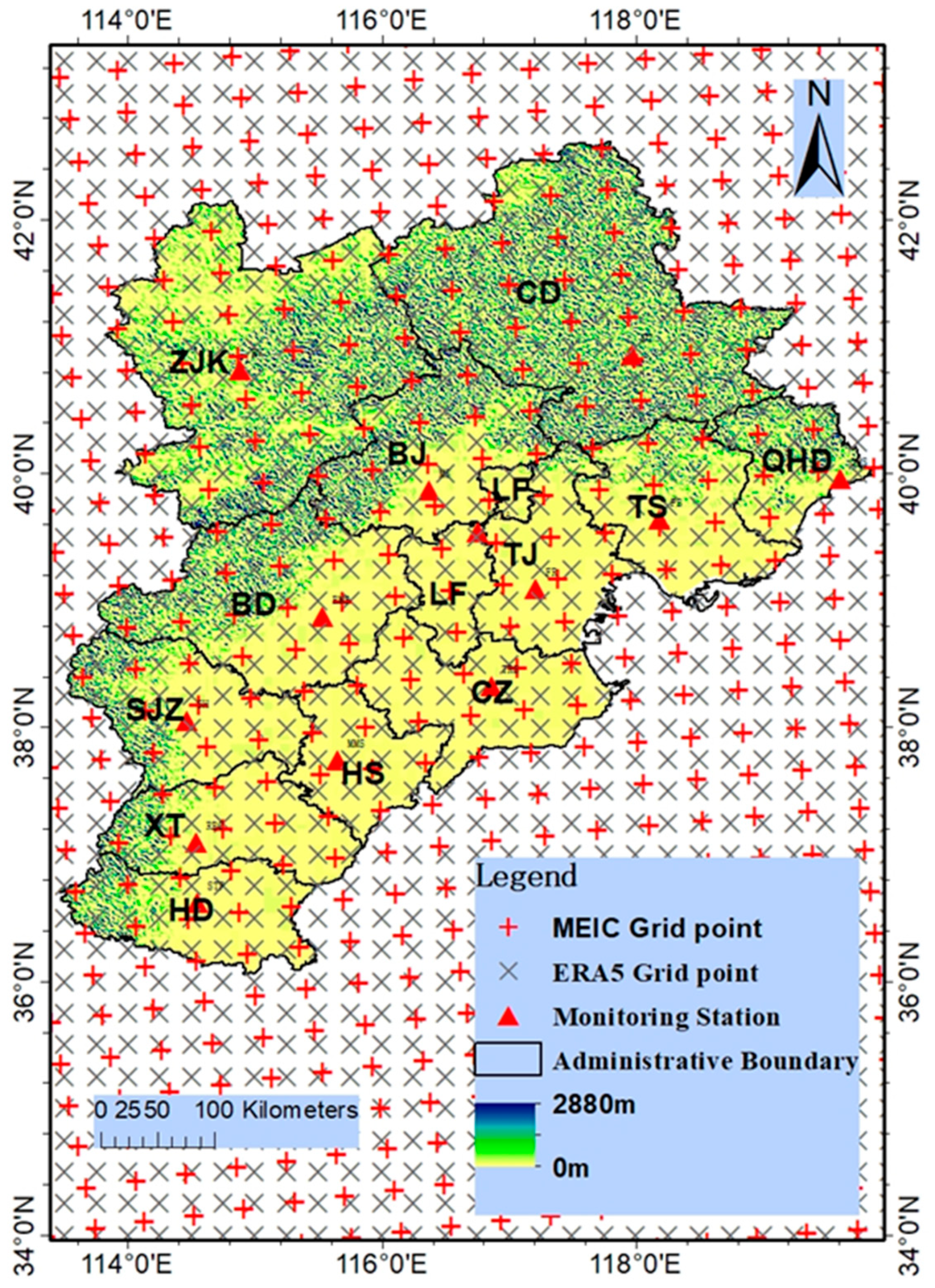
2.1. Research Domain and Period Chosen

This research focuses on the Beijing–Tianjin–Hebei (BTH) region (113.45° E~119.85° E and 36.03° N~42.62° N), encompassing 13 cities: Beijing (BJ), Tianjin (TJ), Shijiazhuang (SJZ), Tangshan (TS), Qinhuangdao (QHD), Handan (HD), Baoding (BD), Zhangjiakou (ZJK), Chengde (CD), Langfang (LF), Cangzhou (CZ), Hengshui (HS), and Xingtai (XT). This region, which spans diverse terrains from the seaside to mountainous areas, constitutes the largest economic hub in northern China, characterized by a high emission density (excluding CD and ZJK). The unique topographic features, variable meteorological fields, and substantial emissions make it prone to elevated PM_2.5 concentrations. Within these cities, the following stations were selected as research targets: Mansu Saigon (MS), Forward Road (FR), Staff Hospital (SH), Property Bureau (PB), Qinhuangdao Monitoring Station (QMS), Sewage Treatment Plant (STP), Baoding Monitoring Station (BMS), Hardware Vault (HV), Development Zone (DZ), North China Institute of Aeronautics (NCIA), Television Relay Station (TRS), Municipal Monitoring Station (MMS), and Road and Bridge Company (RBC). Detailed information can be found in Figure 1.

The study period spanned from 1 January 2016 to 31 December 2017, totaling 17,544 h, during which comprehensive measures were implemented. Figure 2 depicts the monthly PM_2.5 concentrations at the selected stations. Specifically, for HV and DZ, the PM_2.5 concentrations remained below 75 μg/m³ throughout the two-year period. In 2017, the monthly PM_2.5 concentrations at QMS also stayed below the 75 μg/m³ threshold. Conversely, for SH, STP, RBC, BMS, MMS, TRS, and NCIA, the monthly PM_2.5 concentrations exhibited a significant increase from August to December 2017, eventually surpassing 150 μg/m³. The trend observed in the two-year line plot indicates the influence of meteorological characteristics on air quality. Furthermore, notable trough values were observed in May and August 2016, and in April, June, and August 2017, across all stations, indicating the implementation of stringent and timely control measures by the Chinese government in 2017. A comparative analysis revealed that after February 2017, the PM_2.5 concentrations consistently remained below 150 μg/m³, including in December of the same year, indicating the substantial positive impact of the measures. In terms of data training, the selection of 2016 for the training process and 2017 for testing was deemed reasonable.

2.2. Datasets and Processing

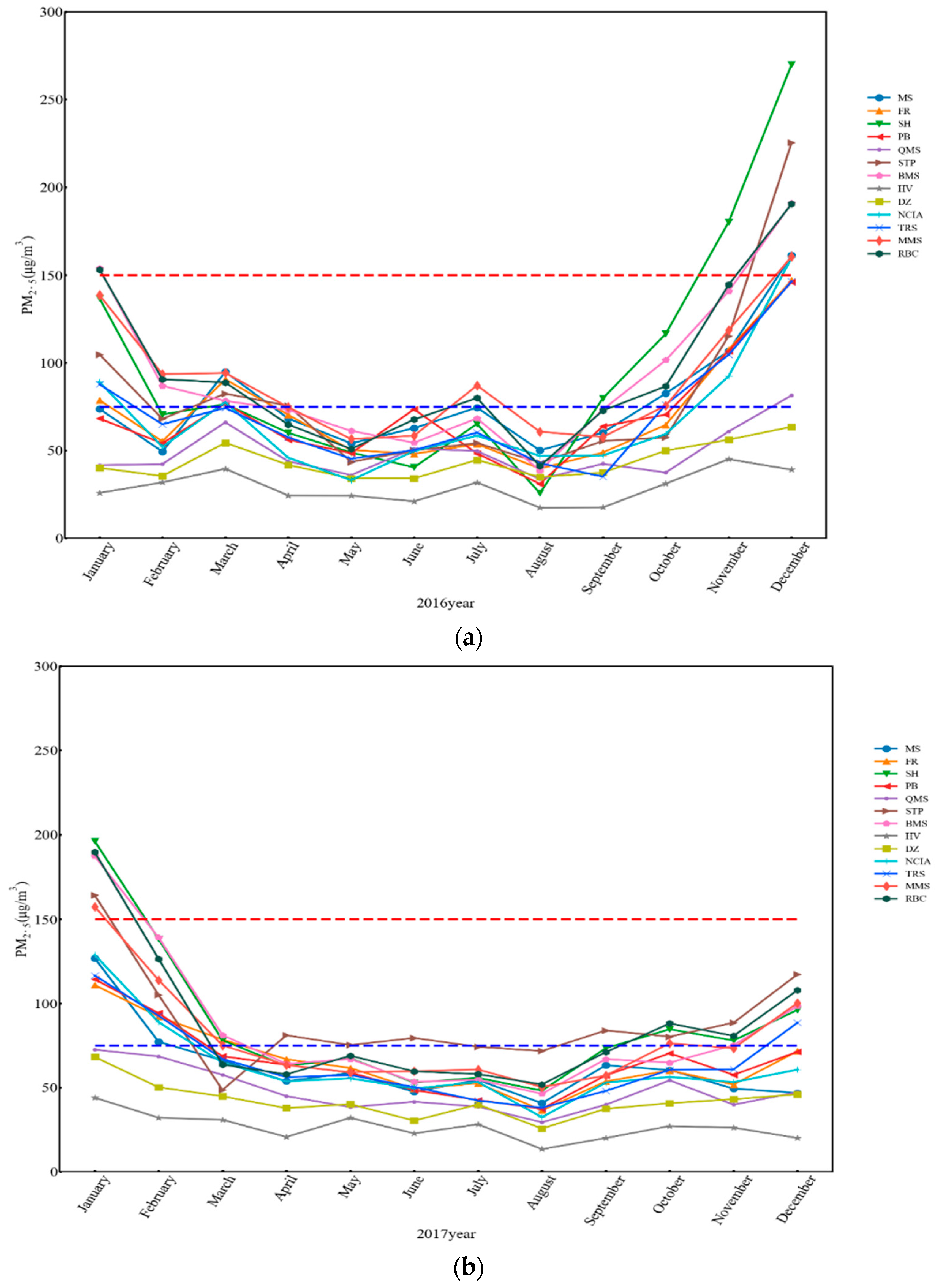
2.2.1. Ground Air Quality Concentration

Hourly ground-level data for six primary air pollutants (PM_2.5, PM₁₀, SO₂, CO, NO₂, and O₃) were obtained from the China National Environmental Monitoring Center for the duration of 1 January 2016 to 31 December 2017. Throughout this period, the hourly air quality monitoring data from all the stations were stored in a MySQL 5.5 database. Subsequently, data from 13 stations in the BTH region were extracted from this database.

2.2.2. ECMWF-ERA5 Meteorological Factors

The meteorological data utilized in this study were obtained from the ECMWF-ERA5 hourly data on single levels and ERA5-Land hourly data from the ECMWF reanalysis, encompassing the entire years of 2016 and 2017. These datasets were acquired at a spatial resolution of 0.25 degree × 0.25 degree. Specifically, the surface pressure (SPRE), relative humidity (RH), 2 m temperature (TMP), as well as the u and v components of wind were selected as input factors for the model. To ensure spatial alignment with the corresponding air quality data, the nearest distance algorithm was employed to calculate the corresponding positions.

Throughout the training process, it was observed that the u and v components of wind exhibited adverse effects on predictions. As a result, in the present study, these components were converted into wind speed (WS) and wind direction (WD) using the following functions:

$$\mathrm{WS}=\sqrt{{\mathrm{u}}^2+{\mathrm{v}}^2}$$

(1)

$$\mathrm{WD}=\{\begin{array}{ll}{\tan }^{-1}\left|\frac{v}{u}\right|,& (\mathrm{u}\ge 0,\mathrm{v}\ge 0)\\ 2\mathsf{\pi }-{\tan }^{-1}\left|\frac{v}{u}\right|,& (\mathrm{u}\ge 0,\mathrm{v}<0)\\ \mathsf{\pi }-{\tan }^{-1}\left|\frac{v}{u}\right|,& (\mathrm{u}<0,\mathrm{v}\ge 0)\\ \mathsf{\pi }+{\tan }^{-1}\left|\frac{v}{u}\right|,& (\mathrm{u}<0,\mathrm{v}<0)\end{array}$$

(2)

where u and v represent horizontal and vertical wind speeds, respectively. Positive u values indicate eastward wind, while negative values indicate westward wind. Similarly, positive v values indicate upward wind, while negative values indicate downward wind.

2.2.3. MEIC Emission Dataset

To accurately procure the emission data for the BTH region, the MEIC version 1.3, encompassing CO, NOx, NO₂, VOCs, NO₂, PM_2.5, PM-coarse, BC, and OC, with a spatial resolution of 0.25 × 0.25 throughout 2016 and 2017, was obtained from its official website. In order to attain a representative distribution of emission characteristics, the SMOKE model was employed to process the data, with spatial and temporal resolutions adjusted to 36 km × 36 km and 1 h, respectively. Moreover, for the species allocation of VOCs, the CB05 chemical mechanism was selected [38,39]. Finally, the nearest distance algorithm was utilized to determine the corresponding positions of the air quality stations.

2.3. Methods and Technical Roadmap

2.3.1. The Structure of the Experimental Model

The LSTM neural network, a derivative of the recurrent neural network (RNN), effectively addresses the issues of gradient explosion and vanishing gradients. In this study, our primary focus was not on the algorithm itself. Instead, the research aimed to develop a system that is capable of utilizing air quality data, meteorological factors, and pollutant emission inventories to forecast future air quality and advance the management of emission pollutants using innovative strategies.

Using a single-layer LSTM model, we assessed the performance of the PM_2.5 concentration prediction. The chosen optimizer and loss function were “Adam” [40] and “MAE”, respectively. Throughout the experiments, the inclusion of additional related features led to an expansion of the design input factors, as outlined in detail in

Table 1. Input variables.

Category	Variables		Unit	Notes
Air quality monitoring dataset		PM2.5, PM10	μg/m3
		SO2, NO2, O3 and CO	mg/m3
ECMWF-ERA5 Meteorological factors	surface pressure (SPRE)		Pa
	relative humidity (RH)		%
	2 m temperature (TMP)		°C
	u component of wind speed(U)		m/s	Eastern direction is positive, western is negative
	v component of wind speed(V)		m/s	Northern direction is positive, southern is negative
Chemical components of MEIC dataset	ALD2, ALDx, BENZENE, CO, ETH, ETHA, EOH, FORM, HONO, IOLE, ISOP, MEOH, NH3, NO, NO2, NVOL, OLE, PAR, SO2, SULF, TERP, TOL		moles/s	CO, NOx, SO2, VOCs, NH3, PM2.5, PM-coarse, BC, and OC are converted to the input variable by SMOKE
	PAL, PCA, PCL, PEC, PFE, PH2O, PK, PMC, UNR, XYL, PMG, PMN, PMOTHER, PNA, PNCOM, PNH4, PNO3, POC, PSI, PSO4, PTI		g/s

.

2.3.2. The Experimental Design and Result Evaluation

In this study, our target for prediction was the PM_2.5 concentration measured at 13 selected monitoring stations. The prediction tests consisted of three datasets: (1) TEST1, which included hourly air quality monitoring data; (2) TEST2, comprising the coupling of TEST1 with ECMWF-ERA5’s meteorological factors; and (3) TEST3, which encompassed the combination of TEST2 with the chemical components of the MEIC emission dataset. To mitigate the inherent randomness in the system, we conducted the tests 100 times and then calculated the average results. Also, to determine the appropriate input variables, we employed the Mann–Kendall test. Detailed information can be seen in Figure 3.

To assess the influence of different datasets and the impact of neuron cells on the prediction accuracy, we designed six experiments utilizing a single-layer LSTM model with an unchanged optimizer and loss function. Experiments 1–3 evaluated the impact of adding different datasets on the PM_2.5 prediction performance. The first experiment focused on the performance of the air quality dataset alone. The second and third experiments added ECMWF-ERA5’s meteorological factors and the chemical components of the MEIC emission dataset coupled with ECMWF-ERA5 meteorological factors, respectively.

To assess the simulated results derived from the aforementioned experiments, we utilized the determination coefficient (R²), mean absolute error (MAE), and root mean square error (RMSE) as statistical criteria. The specific formulations for evaluating these parameters are listed below.

$${\mathrm{R}}^2=1-\frac{{{\displaystyle \sum }}_{i=1}^N{\left(y_i-{\widehat{y}}_i\right)}^2}{{{\displaystyle \sum }}_{i=1}^N{\left(y_i-\overline{y}\right)}^2}$$

(3)

$$\mathrm{MAE}=\frac{1}{N}{{\displaystyle \sum }}_{i=1}^N\left|y_i-{\widehat{y}}_i\right|$$

(4)

$$\mathrm{RMSE}=\sqrt{\frac{1}{N}{{\displaystyle \sum }}_{i=1}^N{\left(y_i-{\widehat{y}}_i\right)}^2}$$

(5)

where $y_i$ and ${\widehat{y}}_i$ represent the values of the monitoring data and predicted data at i time, respectively, $\overline{y}$ denotes the mean value of the monitoring data, and N illustrates the number of samples.

3. Results and Discussion

3.1. Mann–Kendall Correlation for Input Variables

In order to obtain the appropriate input variables, input feature selection is a key procedure. In this research, the Mann–Kendall test was chosen to evaluate the relationship among air quality, ECMWF-ERA5’s meteorological factors, and the chemical components of the MEIC emission dataset and then determine the number of input variables. From the datasets mentioned above, we can see that there were a total of fifty-four input features in Table 1, namely, six, five, and forty-three, corresponding to the three datasets, respectively. During the process, the relationship between the t-th PM_2.5 and (t − 1)-th variables are tested by the Mann–Kendall correlation coefficient, where ** and * represent 0.01 and 0.05 levels of significance, respectively. We set a Kendall correlation coefficient absolute value > 0.08 as the threshold value to choose the appropriate features (Table 1).

The air quality dataset shows that PM_2.5, PM₁₀, CO, SO₂, and NO₂ have a positive influence on the performance of the PM_2.5 prediction in the next time step. The highest influence is observed for PM_2.5, with correlation coefficients ranging from 0.756 to 0.865, followed by PM₁₀, CO, SO₂, and NO₂. Conversely, O₃ has a negative influence, with correlation coefficients ranging from 0.056 to 0.136. The influence of the dataset is relatively stable. Regarding the ECMWF-ERA5 meteorological factors, RH and WS have a consistent influence. RH has a positive impact, with correlation coefficients ranging from 0.134 to 0.317, while WS has a negative impact, with coefficients ranging from 0.129 to 0.238. The influence of the remaining factors (SPRE, TMP, and WD) is unstable. WD, for example, did not pass the Kendall 0.01 test on PB and had positive functions for the HV, DZ, and SH factors. RH is conducive to the formation of PM_2.5, while WS is favorable for PM_2.5 diffusion. Therefore, RH and WS perform well in predicting air quality. The Mann–Kendall test results for chemical species show that sixteen species listed in

Table 2. Kendall test results of different datasets for PM_2.5 concentration prediction.

(a) Air quality monitoring dataset and ECMWF-ERA5 meteorological factors.
Stations	PM2.5 (t − 1)		PM10 (t − 1)		CO (t − 1)	O3 (t − 1)	NO2 (t − 1)		SO2 (t − 1)	SPRE (t − 1)	TMP (t − 1)		RH (t − 1)	WD (t − 1)		WS (t − 1)
MS	0.847		0.66		0.65	−0.161	0.47		0.313	−0.081	-		0.317	-		−0.187
FR	0.829		0.66		0.522	−0.205	0.429		0.392	-	−0.082		0.177	−0.092		−0.161
SH	0.852		0.689		0.615	−0.245	0.476		0.399	0.152	−0.235		0.198	-		−0.168
PB	0.837		0.69		0.391	−0.24	0.509		0.405	-	−0.098		0.242	-		−0.179
QMS	0.844		0.69		0.492	−0.136	0.402		0.307		-		0.242	−0.15		−0.132
STP	0.848		0.673		0.463	−0.269	0.402		0.295	0.089	−0.167		0.174			−0.169
BMS	0.86		0.722		0.594	−0.315	0.504		0.426	0.13	−0.229		0.152	-		−0.188
HV	0.756		0.564		0.535		0.519		0.349		-		0.134	0.178		−0.129
DZ	0.844		0.705		0.558	−0.175	0.514		0.394	-	-		0.253	-		−0.206
NCIA	0.865		0.723		0.605	−0.225	0.416		0.443	-			0.292	-		−0.238
TRS	0.837		0.668		0.486	−0.237	0.43		0.332		−0.172		0.161			−0.161
MMS	0.849		0.63		0.526	−0.269	0.408		0.324	0.097	−0.182		0.188	-		−0.155
RBC	0.836		0.674		0.536	−0.283	0.469		0.342	0.136	−0.216		0.154	-		−0.146
(b) Kendall test of MEIC chemical component dataset for PM2.5 concentration prediction.
Stations	XYL (t − 1)	PNCOM (t − 1)	POC (t − 1)	ALD2 (t − 1)	ALDX (t − 1)	BENZENE (t − 1)	ETOH (t − 1)	FORM (t − 1)	ISOP (t − 1)	MEOH (t − 1)	NVOL (t − 1)	PAR (t − 1)	NO (t − 1)	NO2 (t − 1)	HONO (t − 1)	NH3 (t − 1)
	unit: g/s			unit: moles/s
MS	-	-	-	-	-	-	-	-	-	-	-	-	-	-	-	−0.115
FR	-	-	-	-	-	-	-	-	-	-	-	-	-	-	−0.085	-
SH	-	-	-	0.090	0.110	0.087	-	-	0.089	-	-	-			-	−0.188
PB	-	-	-	-	-	-	-	-	-	-	-	-			−0.89
QMS	-	-	-	-	-	-	-	-	-	-	-				-	−0.108
STP	-	-	-	-	-	0.086	-	-	-	0.080	0.109	-	-	-	-	−0.167
BMS	−0.083	-	-	-	-	-	−0.118	-	-	-	-	−0.081	−0.113	-0.115	-0.092	−0.174
HV	-	-	-	-	-	-	-	-	-	-	-	-	−0.103	-	-
DZ	-	-	-	-	-	-	-	-	-	-	-				-	−0.098
NCIA	-	-	-	-	-	-	-	-	-	-	-				-	−0.107
TRS	-	-	-	-	-	-	−0.102	-	-	-	-		−0.099	-0.100	−0.089	−0.133
MMS	-	-	-	-	-	-	−0.089	-	-	-	-		−0.086	-0.087	−0.088	−0.149
RBC	-	0.089	0.086	0.092	0.103	-	-	0.086	0.092	-	-	-				−0.204

Notes: The newlines represent that the results did not pass the Mann–Kendall test. And the blank lines mean that the variables passed the test, but the values were too small to discard.

passed the test at the 13 stations. NO₂ passed at ten stations, and HONO passed at five stations, indicating that these chemical components are useful for predicting PM_2.5 concentrations.

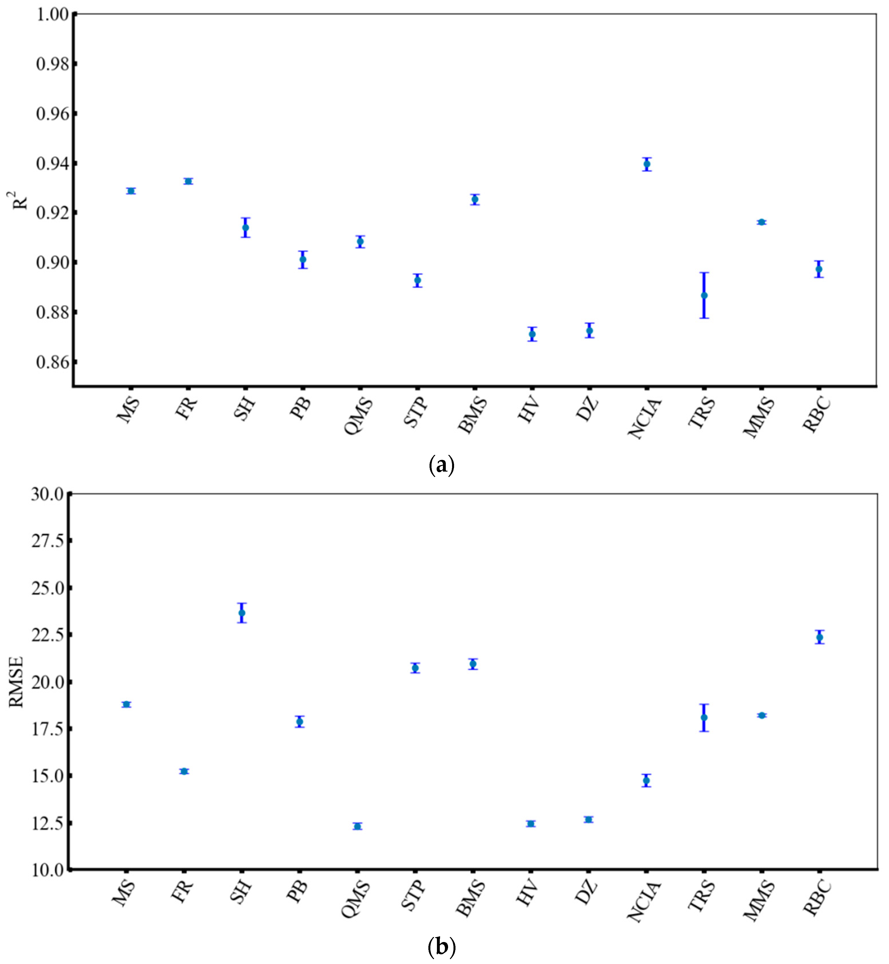
3.2. Prediction Performance of the Next-Hour PM_2.5 Concentration

To assess the prediction accuracy of the proposed model in forecasting the PM_2.5 concentration using air quality data, hourly air quality forecasting was conducted. Throughout the training period using the year of 2016, there were slight changes in the standard deviations of R² and RMSE. The mean values of R² and RMSE were 0.907 ± 0.0029 and 17.54 ± 0.273, respectively. For instance, the maximum standard deviations of R² and RMSE for TRS were 0.009 and 0.725. Additionally, we observed a range of values for R² between 0.871 and 0.940, and for RMSE between 12.309 and 23.660. This information is presented in Figure 4, where the predicted results from the 13 stations demonstrate a strong consistency. Consequently, we have confidence that both underfitting and overfitting did not occur throughout the modeling run (Figure 5). Therefore, the model is deemed capable of effectively predicting PM_2.5 concentrations within the BTH region.

The results based on the four seasons and different pollution levels were analyzed to evaluate the forecasting performance of the model. As shown in

Table 3. PM_2.5 prediction performance of air quality dataset in different seasons and levels.

(a) Performance evaluation in different seasons.
Stations	Spring		Summer		Autumn		Winter
	MAE	R2	MAE	R2	MAE	R2	MAE	R2
MS	9.743	0.916	7.945	0.832	6.997	0.941	11.480	0.932
FR	10.019	0.915	7.980	0.801	7.262	0.913	11.324	0.944
SH	16.265	0.823	13.491	0.566	13.964	0.848	19.078	0.932
PB	11.869	0.803	7.211	0.754	8.490	0.900	13.069	0.928
QMS	8.953	0.845	7.451	0.829	6.500	0.911	8.962	0.930
STP	11.146	0.843	11.835	0.724	10.810	0.863	17.615	0.898
BMS	10.715	0.897	8.640	0.718	8.247	0.907	18.104	0.916
HV	7.170	0.853	6.869	0.719	5.223	0.869	7.101	0.911
DZ	5.320	0.911	4.821	0.898	5.015	0.899	7.774	0.833
NCIA	9.019	0.905	6.751	0.839	7.194	0.916	11.494	0.952
TRS	12.649	0.855	10.770	0.640	11.526	0.814	15.070	0.902
MMS	9.146	0.831	7.504	0.831	7.612	0.911	15.835	0.916
RBC	12.965	0.791	11.246	0.663	12.316	0.847	20.398	0.898
Average	10.383	0.861	8.655	0.755	8.551	0.888	13.639	0.915
(b) Performance evaluation at different levels.
Stations	Level-1 (0–75 μg/m3)			Level-2 (75–150 μg/m3)		Level-3 (>150 μg/m3)
	MAE		R2	MAE	R2	MAE		R2
MS	7.271		0.430	10.483	0.396	20.686		0.873
FR	7.493		0.663	10.443	0.298	19.728		0.756
SH	12.812		0.256	18.008	0.464	24.236		0.846
PB	7.270		0.479	15.685	0.165	23.487		0.626
QMS	6.491		0.649	13.843	0.136	18.504		0.722
STP	9.131		0.101	14.498	0.010	22.212		0.689
BMS	7.520		0.359	13.893	0.068	24.379		0.801
HV	5.471		0.738	15.572	0.114	43.651		0.384
DZ	4.295		0.819	13.546	0.146	30.787		0.297
NCIA	6.390		0.654	13.286	0.157	19.091		0.820
TRS	10.859		0.170	14.858	0.068	23.269		0.681
MMS	6.324		0.461	12.946	0.190	24.189		0.705
RBC	10.488		0.045	17.154	0.257	24.432		0.753
Average	7.832		0.448	14.170	0.190	24.512		0.689

a, good performances were achieved by the model. The average R² values appeared in the sequence of summer (0.755), spring (0.861), autumn (0.888), and winter (0.915), with the best performance presented by winter. Additionally, it is noted that we can capture the high pollution episodes in winter (Table 3b). Specifically, the PM2.5 levels are divided into low (0~75 μg/m³), middle (75–150 μg/m³), and high (>150 μg/m³), and the model performed well for the majority of the stations under the high PM_2.5 pollution level. This is because the PM_2.5 concentration for these stations throughout 2016 and 2017 remained at a high concentration, featuring a high pollution frequency. Correspondingly, the average R², MAE, and RMSE for the low PM2.5 level were 0.464, 7.417, and 12.102, respectively. These values were found to be lower than the corresponding metrics for the high PM_2.5 concentration level, which were 0.689, 24.512, and 40.406, respectively.

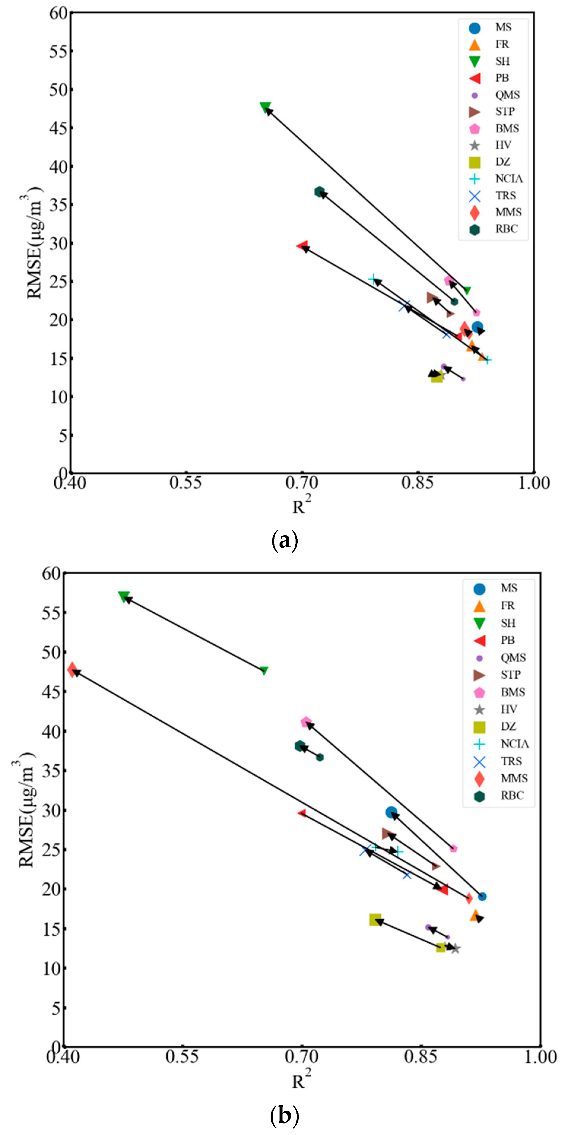
3.3. Evaluation Performance of Air Monitoring, Meteorological Factors, and Emission Inventory on PM_2.5 Prediction

By employing the same approach as TEST1 did, an assessment was conducted on the predictive capabilities of TEST2 and TEST3. The R², MAE, and RMSE values obtained from the TEST1 simulation were 0.907, 10.349, and 17.550, respectively, which were correspondingly 0.833, 16.577, and 23.297 for the TEST2 simulation and 0.755, 21.584, and 28.554 for TEST3 (seen in Figure 6), respectively. Notably, significant improvements were not achieved by introducing meteorological factors and the MEIC emission dataset. The reason for this phenomenon is attributed to discrepancies in the temporal emission characteristics of the emission inventory. The employment of uniform temporal allocation coefficients results in an inadequate representation of the temporal emission characteristics across different regions, consequently constraining the predictive accuracy [41]. Regional heterogeneity in meteorology on a large scale can also be responsible for this phenomenon, resulting in improved predictive performance for some meteorological sites, while others experience less improvement [42]. Additionally, the terrain of the observation sites, located in coastal, plain, and mountainous areas, indicates that the differences in terrain have a certain impact on or interference with the predictive performance of atmospheric pollution [43]. Thus, in future regional air quality forecasting processes, it is necessary to fully consider the effects of terrain variations, heterogeneity in meteorological conditions, and differences in emission inventory emission characteristics.

Based on the above discussion, the R², MAE, and RMSE values obtained from TEST3 ranged from 0.411 to 0.918, 7.329 to 46.787, and 12.827 to 56.960, respectively. It is obvious that the prediction performance of PM_2.5 concentrations was superior to knowledge-driven models that also utilized meteorological models, such as the Weather Research and Forecasting model (WRF), to forecast air quality by using the air pollutants [44]. When using air monitoring quality datasets and ECMWF-ERA5 meteorological factors to forecast PM_2.5 concentrations, we achieved a timely hourly prediction. We noted an improvement in prediction performance for the three stations (NCIA, HV, and PB), possibly due to the alignment of the temporal profiles of chemical components with the true situation. Thus, employing the same temporal profile may not be suitable for addressing the emission inventory in a large area. This implies that different regional temporal profiles in the emission inventory could enhance the performance of knowledge-driven models in air quality prediction.

4. Conclusions

In this research, a single-layer LSTM model was constructed to evaluate the influence of meteorological factors from ECMWF-ERA5 and the emission inventory from MEIC. The results showed that the air quality dataset can achieve the best performance, reaching an R² of 0.907 on average in the chosen 13 stations, while for different seasons and levels, winter and a high level are superior to the other seasons and levels on average. The ECMWF-ERA5 and MEIC datasets can equally obtain an approximate prediction performance, which is perhaps due to the chosen meteorological factors of ECMWF- ERA5 and the chemical components of the MEIC dataset, which cannot accurately reflect the spatial and temporal characteristics with the changing PM_2.5 trend, but is still better than knowledge-driven model for long-term prediction.

The contribution of this work was to construct a new system which included both the external and internal causes of air pollution using an LSTM model, such as meteorological factors and the local emission inventory, which were commonly used in knowledge-driven models. Although the prediction performance of the new method did not improve greatly, the results were still superior to those of knowledge-driven models. Moreover, this research provided an idea for optimizing knowledge-driven models by improving the accuracy of the prediction performance. In addition, the proposed method had a certain capacity to predict the regional air quality of each monitoring station and manage the local pollutant emission for the future reduction plan.

References

1. Shao, M.; Dai, Q.; Yu, Z.; Zhang, Y.; Xie, M.; Feng, Y. Responses in PM2.5 and its chemical components to typical unfavorable meteorological events in the suburban area of Tianjin, China. Sci. Total Environ. 2021, 788, 147814. [Google Scholar] [CrossRef]
2. Zhao, X.; Wang, G.; Wang, S.; Zhao, N.; Zhang, M.; Yue, W. Impacts of COVID-19 on air quality in mid-eastern China: An insight into meteorology and emissions. Atmos. Environ. 2021, 266, 118750. [Google Scholar] [CrossRef] [PubMed]
3. Zhang, Y.; Ding, A.; Mao, H.; Nie, W.; Zhou, D.; Liu, L.; Huang, X.; Fu, C. Impact of synoptic weather patterns and inter-decadal climate variability on air quality in the North China Plain during 1980–2013. Atmos. Environ. 2016, 124, 119–128. [Google Scholar] [CrossRef]
4. Wang, Y.; Ying, Q.; Hu, J.; Zhang, H. Spatial and temporal variations of six criteria air pollutants in 31 provincial capital cities in China during 2013–2014. Environ. Int. 2014, 73, 413–422. [Google Scholar] [CrossRef] [PubMed]
5. Kim, K.W.; Kim, Y.J. Characteristics of visibility-impairing aerosol observed during the routine monitoring periods in Gwangju, Korea. Atmos. Environ. 2018, 193, 40–56. [Google Scholar] [CrossRef]
6. Cabrera López, C.; Urrutia Landa, I.; Jiménez-Ruiz, C.A. SEPAR’s year: Air quality. SEPAR statement on climate change. Arch. Bronconeumol. (Engl. Ed.) 2021, 57, 313–314. [Google Scholar] [CrossRef]
7. Sá, E.; Martins, H.; Ferreira, J.; Marta-Almeida, M.; Rocha, A.; Carvalho, A.; Freitas, S.; Borrego, C. Climate change and pollutant emissions impacts on air quality in 2050 over Portugal. Atmos. Environ. 2016, 131, 209–224. [Google Scholar] [CrossRef]
8. Chen, H.; Li, Q.; Kaufman, J.S.; Wang, J.; Copes, R.; Su, Y.; Benmarhnia, T. Effect of air quality alerts on human health: A regression discontinuity analysis in Toronto, Canada. Lancet Planet. Health 2018, 2, e19–e26. [Google Scholar] [CrossRef]
9. Fattore, E.; Paiano, V.; Borgini, A.; Tittarelli, A.; Bertoldi, M.; Crosignani, P.; Fanelli, R. Human health risk in relation to air quality in two municipalities in an industrialized area of Northern Italy. Environ. Res. 2011, 111, 1321–1327. [Google Scholar] [CrossRef]
10. Liao, Z.; Gao, M.; Sun, J.; Fan, S. The impact of synoptic circulation on air quality and pollution-related human health in the Yangtze River Delta region. Sci. Total Environ. 2017, 607–608, 838–846. [Google Scholar] [CrossRef]
11. Nowak, D.J.; Hirabayashi, S.; Doyle, M.; McGovern, M.; Pasher, J. Air pollution removal by urban forests in Canada and its effect on air quality and human health. Urban For. Urban Green. 2018, 29, 40–48. [Google Scholar] [CrossRef]
12. Teoldi, F.; Lodi, M.; Benfenati, E.; Colombo, A.; Baderna, D. Air quality in the Olona Valley and in vitro human health effects. Sci. Total Environ. 2017, 579, 1929–1939. [Google Scholar] [CrossRef]
13. Lin, J.; Long, C.; Yi, C. Has central environmental protection inspection improved air quality? Evidence from 291 Chinese cities. Environ. Impact Assess. 2021, 90, 106621. [Google Scholar] [CrossRef]
14. Liu, Z.; Xue, W.; Ni, X.; Qi, Z.; Zhang, Q.; Wang, J. Fund gap to high air quality in China: A cost evaluation for PM2.5 abatement based on the Air Pollution Prevention and control Action Plan. J. Clean. Prod. 2021, 319, 128715. [Google Scholar] [CrossRef]
15. Xue, W.; Wang, J.; Niu, H.; Yang, J.; Han, B.; Lei, Y.; Chen, H.; Jiang, C. Assessment of air quality improvement effect under the National Total Emission Control Program during the Twelfth National Five-Year Plan in China. Atmos. Environ. 2013, 68, 74–81. [Google Scholar] [CrossRef]
16. Cai, W.-J.; Wang, H.-W.; Wu, C.-L.; Lu, K.-F.; Peng, Z.-R.; He, H.-D. Characterizing the interruption-recovery patterns of urban air pollution under the COVID-19 lockdown in China. Build. Environ. 2021, 205, 108231. [Google Scholar] [CrossRef] [PubMed]
17. Huang, G.; Blangiardo, M.; Brown, P.E.; Pirani, M. Long-term exposure to air pollution and COVID-19 incidence: A multi-country study. Spat. Spatio-Temporal 2021, 39, 100443. [Google Scholar] [CrossRef] [PubMed]
18. Herwehe, J.A.; Otte, T.L.; Mathur, R.; Rao, S.T. Diagnostic analysis of ozone concentrations simulated by two regional-scale air quality models. Atmos. Environ. 2011, 45, 5957–5969. [Google Scholar] [CrossRef]
19. José, R.S.; Pérez, J.L.; Morant, J.L.; González, R.M. Elevated PM10 and PM2.5 concentrations in Europe: A model experiment with MM5-CMAQ and WRF-CHEM. WIT Trans. Ecol. Environ. 2018, 116, 3–12. [Google Scholar]
20. Lee, M.; Lin, L.; Chen, C.-Y.; Tsao, Y.; Yao, T.-H.; Fei, M.-H.; Fang, S.-H. Forecasting air quality in Taiwan by using machine learning. Sci. Rep. 2020, 10, 4153. [Google Scholar] [CrossRef]
21. Kaginalkar, A.; Kumar, S.; Gargava, P.; Niyogi, D. Review of urban computing in air quality management as smart city service: An integrated IoT, AI, and cloud technology perspective. Urban Clim. 2021, 39, 100972. [Google Scholar] [CrossRef]
22. Kalia, P.; Ansari, M.A. IOT based air quality and particulate matter concentration monitoring system. Mater. Today Proc. 2020, 32, 468–475. [Google Scholar] [CrossRef]
23. Senthilkumar, R.; Venkatakrishnan, P.; Balaji, N. Intelligent based novel embedded system based IoT enabled air pollution monitoring system. Microprocess. Microsy 2020, 77, 103172. [Google Scholar] [CrossRef]
24. Gao, C.; Li, S.; Liu, M.; Zhang, F.; Achal, V.; Tu, Y.; Zhang, S.; Cai, C. Impact of the COVID-19 pandemic on air pollution in Chinese megacities from the perspective of traffic volume and meteorological factors. Sci. Total Environ. 2021, 773, 145545. [Google Scholar] [CrossRef] [PubMed]
25. Ma, T.; Duan, F.; He, K.; Qin, Y.; Tong, D.; Geng, G.; Liu, X.; Li, H.; Yang, S.; Ye, S.; et al. Air pollution characteristics and their relationship with emissions and meteorology in the Yangtze River Delta region during 2014–2016. J. Environ. Sci 2019, 83, 8–20. [Google Scholar] [CrossRef]
26. Ulpiani, G.; Ranzi, G.; Santamouris, M. Local synergies and antagonisms between meteorological factors and air pollution: A 15-year comprehensive study in the Sydney region. Sci. Total Environ. 2021, 788, 147783. [Google Scholar] [CrossRef] [PubMed]
27. Jiang, Q.; Li, W.; Fan, Z.; He, X.; Sun, W.; Chen, S.; Wen, J.; Gao, J.; Wang, J. Evaluation of the ERA5 reanalysis precipitation dataset over Chinese Mainland. J. Hydrol. 2021, 595, 125660. [Google Scholar] [CrossRef]
28. Zhang, S.-Q.; Ren, G.-Y.; Ren, Y.-Y.; Zhang, Y.-X.; Xue, X.-Y. Comprehensive evaluation of surface air temperature reanalysis over China against urbanization-bias-adjusted observations. Adv. Clim. Chang. Res. 2021, 12, 783–794. [Google Scholar] [CrossRef]
29. Zhang, L.; Zhao, T.L.; Gong, S.L.; Kong, S.F.; Tang, L.L.; Liu, D.Y.; Wang, Y.W.; Jin, L.J.; Shan, Y.P.; Tan, C.H.; et al. Updated emission inventories of power plants in simulating air quality during haze periods over East China. Atmos. Chem. Phys. 2018, 18, 2065–2079. [Google Scholar] [CrossRef]
30. Chen, D.; Tian, X.; Lang, J.; Zhou, Y.; Li, Y.; Guo, X.; Wang, W.; Liu, B. The impact of ship emissions on PM2.5 and the deposition of nitrogen and sulfur in Yangtze River Delta, China. Sci. Total Environ. 2019, 649, 1609–1619. [Google Scholar] [CrossRef]
31. Chauhan, R.; Kaur, H.; Alankar, B. Air quality forecast using convolutional Neural Network for sustainable development in urban environments. Sustain. Cities Soc. 2021, 75, 103239. [Google Scholar] [CrossRef]
32. Masood, A.; Ahmad, K. A review on emerging artificial intelligence (AI) techniques for air pollution forecasting: Fundamentals, application and performance. J. Clean. Prod. 2021, 322, 129072. [Google Scholar] [CrossRef]
33. Sharma, E.; Deo, R.C.; Prasad, R.; Parisi, A.V. A hybrid air quality early-warning framework: An hourly forecasting model with online sequential extreme learning machines and empirical mode decomposition algorithms. Sci. Total Environ. 2020, 709, 135934. [Google Scholar] [CrossRef] [PubMed]
34. Singh, D.; Dahiya, M.; Kumar, R.; Nanda, C. Sensors and systems for air quality assessment monitoring and management: A review. J. Environ. Manag. 2021, 289, 112510. [Google Scholar] [CrossRef] [PubMed]
35. Han, S.; Dong, H.; Teng, X.; Li, X.; Wang, X. Correlational graph attention-based Long Short-Term Memory network for multivariate time series prediction. Appl. Soft Comput. 2021, 106, 107377. [Google Scholar] [CrossRef]
36. Seng, D.; Zhang, Q.; Zhang, X.; Chen, G.; Chen, X. Spatiotemporal prediction of air quality based on LSTM neural network. Alex. Eng. J. 2021, 60, 2021–2032. [Google Scholar] [CrossRef]
37. Zhao, J.; Deng, F.; Cai, Y.; Chen, J. Long short-term memory—Fully connected (LSTM-FC) neural network for PM2.5 concentration prediction. Chemosphere 2019, 220, 486–492. [Google Scholar] [CrossRef]
38. Heo, G.; McDonald-Buller, E.; Carter, W.P.L.; Yarwood, G.; Whitten, G.Z.; Allen, D.T. Modeling ozone formation from alkene reactions using the Carbon Bond chemical mechanism. Atmos. Environ. 2012, 59, 141–150. [Google Scholar] [CrossRef]
39. Luecken, D.J.; Phillips, S.; Sarwar, G.; Jang, C. Effects of using the CB05 vs. SAPRC99 vs. CB4 chemical mechanism on model predictions: Ozone and gas-phase photochemical precursor concentrations. Atmos. Environ. 2008, 42, 5805–5820. [Google Scholar] [CrossRef]
40. Shahade, A.K.; Walse, K.H.; Thakare, V.M.; Atique, M. Multi-lingual opinion mining for social media discourses: An approach using deep learning based hybrid fine-tuned smith algorithm with adam optimizer. Int. J. Inf. Manag. Data Insights 2023, 3, 100182. [Google Scholar] [CrossRef]
41. Zhong, Z.M.; Zheng, J.Y.; Zhu, M.N.; Huang, Z.J.; Zhang, Z.W.; Jia, G.L.; Wang, X.L.; Bian, Y.H.; Wang, Y.L.; Li, N. Recent developments of anthropogenic air pollutant emission inventories in Guangdong province, China. Sci. Total Environ. 2018, 627, 1080–1092. [Google Scholar] [CrossRef] [PubMed]
42. Li, X.; Wu, J.R.; Elser, M.; Feng, T.; Cao, J.J.; El-Haddad, I.; Huang, R.J.; Tie, X.X.; Prévôt, A.S.H.; Li, G.H. Contributions of residential coal combustion to the air quality in Beijing-Tianjin-Hebei (BTH), China: A case study. Atmos. Chem. Phys. 2018, 18, 10675–10691. [Google Scholar] [CrossRef]
43. Kotake, S.; Sano, T. Simulation-model of air-pollution in complex terrains including streets and buildings. Atmos. Environ. 1981, 15, 1001–1009. [Google Scholar] [CrossRef]
44. Song, S.F.; Zhang, X.Z.; Gao, Z.B.; Yan, X.D. Evaluation of atmospheric circulations for dynamic downscaling in CMIP6 models over East Asia. Clim. Dynam 2022, 60, 2437–2458. [Google Scholar] [CrossRef]
Figure 1. Study area.
Environments 11 00107 g001
Figure 2. Two years of monthly PM2.5 concentrations in the 13 monitoring stations in the BTH region. The blue dotted line (lower one) represents the 75 μg/m3 concentration level and the red line (upper one) represents the 150 μg/m3 concentration level. (a) represents the air quality situation in 2016, and (b) represents the air quality situation in 2017.
Environments 11 00107 g002
Figure 3. Technical roadmap.
Environments 11 00107 g003
Figure 4. Comparison of forecasting performance among chosen 13 stations.
Environments 11 00107 g004
Figure 5. STD of (a) R2 and (b) RMSE in chosen 13 stations based on 100 rounds of prediction.
Environments 11 00107 g005
Figure 6. An evaluation of the performance of the PM2.5 concentration with different datasets. The smaller symbols represent the prediction performance of the air quality dataset, and the bigger ones represent the impact of adding the ECMWF-ERA5 meteorological factors dataset, ECMWF-ERA5 and meteorological factors, and MEIC chemical components dataset, respectively. (a) The comparative performance of air quality with and without the ECMWF-ERA5 meteorological factors dataset; (b) the comparative performance of air quality and ECMWF-ERA5 meteorological factors without and with the chemical components of the MEIC dataset.
Environments 11 00107 g006