
A Method to Quantify the Drainage Basin Contributions to Transitional Water Bodies: Numerical Modeling Applied to the Case Study of Venice Lagoon

 , , ,
, , ,  ,
, 
Abstract
:1. Introduction
2. Materials and Methods
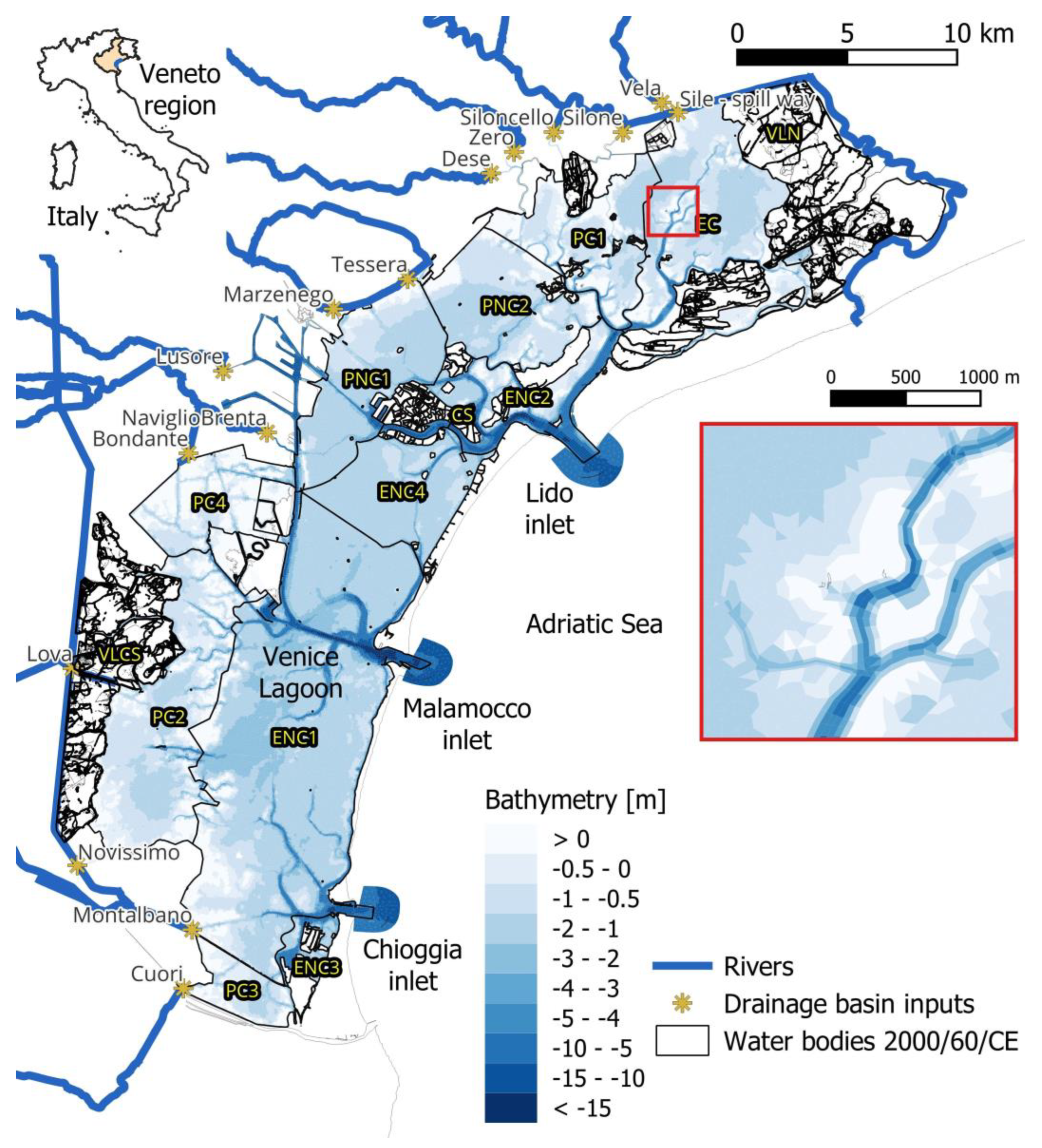
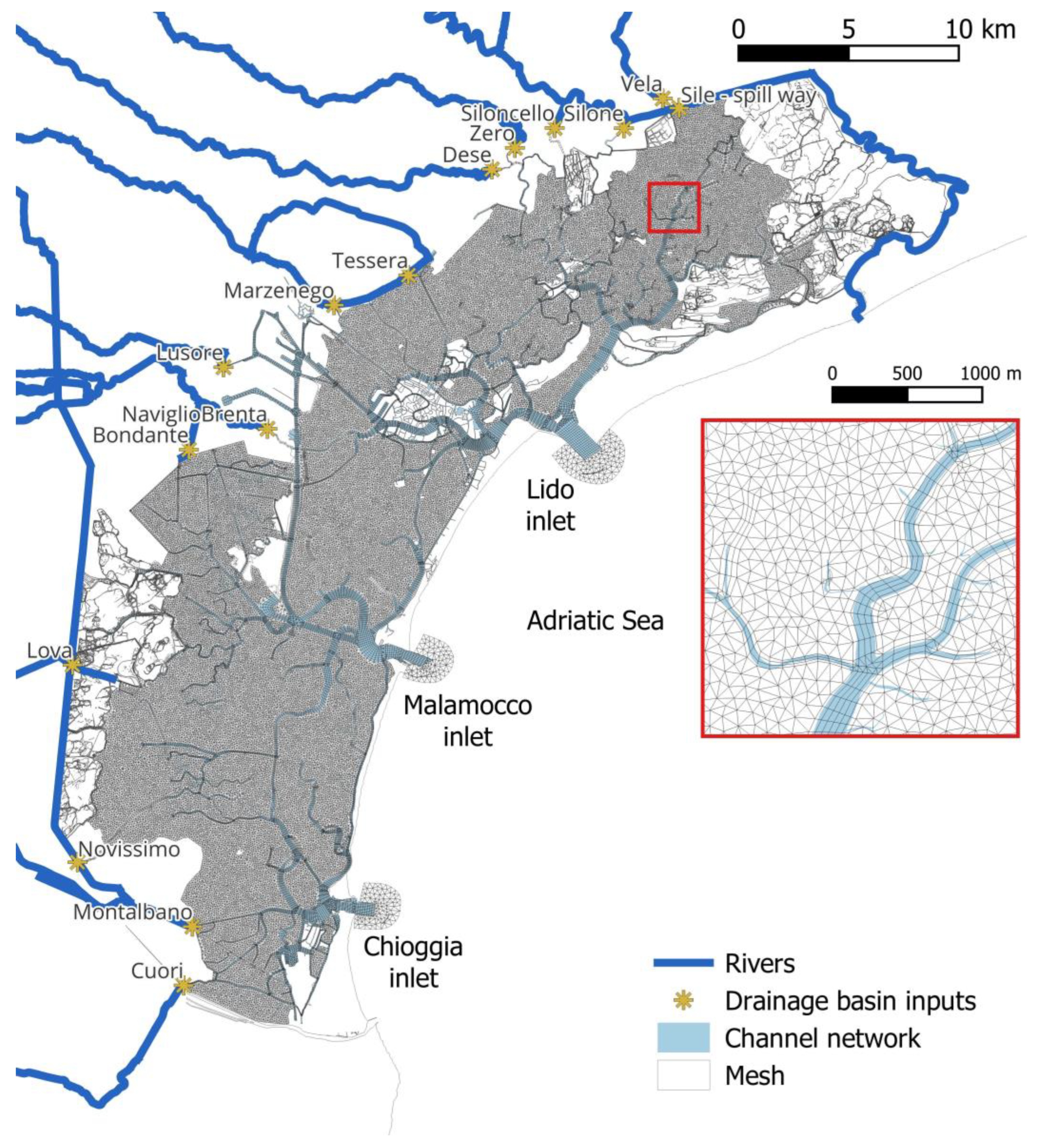
2.1. Numerical Model Setup
2.2. Data Analysis
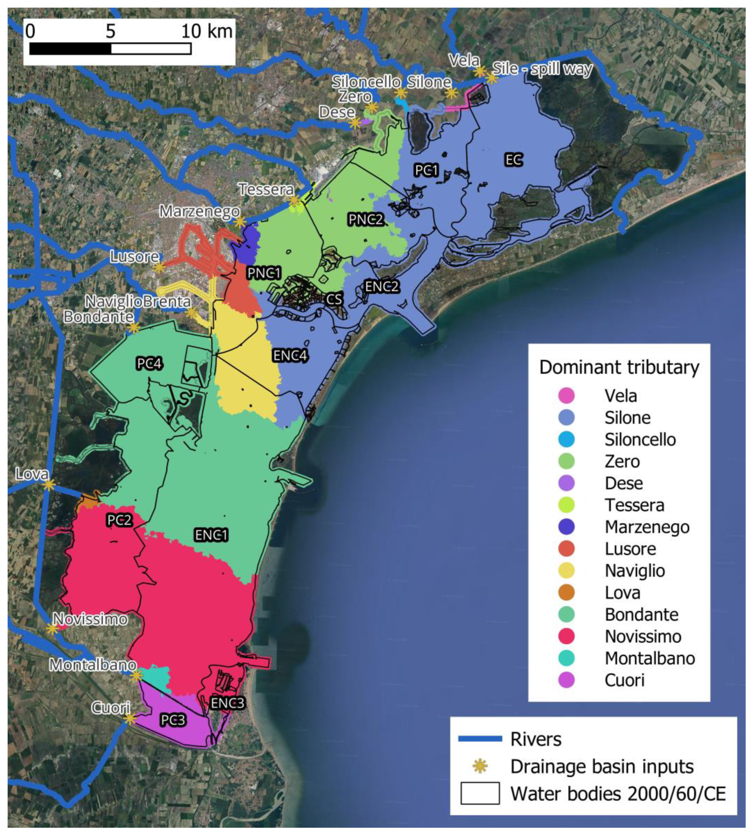
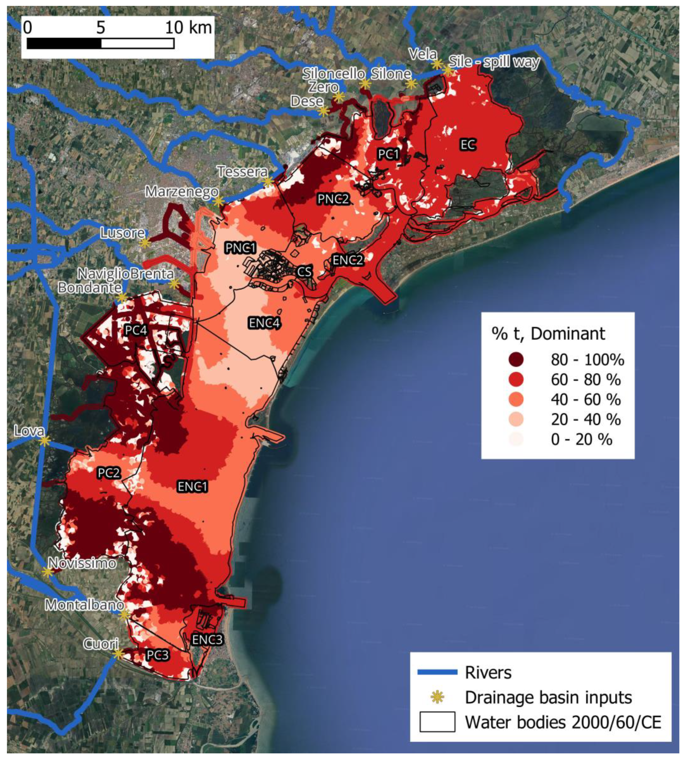
3. Results
4. Discussion and Conclusions
Author Contributions
Funding
Data Availability Statement
Acknowledgments
Conflicts of Interest
List of Abbreviations
References
- De Wit, R. Biodiversity of coastal lagoon ecosystems and their vulnerability to global change. In Ecosystems Biodiversity; Grillo, O., Venore, G., Eds.; InTech Open Access Publisher: London, UK, 2011; pp. 29–40. [Google Scholar]
- Munaron, D.; Tapie, N.; Budzinski, H.; Andral, B.; Gonzalez, J.-L. Alkylphenols and pesticides in Mediterranean coastal waters: Results from a pilot survey using passive samplers. Estuar. Coast. Shelf Sci. 2012, 114, 82–92. [Google Scholar] [CrossRef]
- Smith, S.V.; Swaney, D.P.; Talaue-McManus, L.; Bartley, J.D.; Sandhei, P.T.; McLaughlin, C.J.; Dupra, V.C.; Crossland, C.J.; Buddemeier, R.W.; Maxwell, B.A.; et al. Humans, hydrology, and the distribution of inorganic nutrient loading to the ocean. BioScience 2003, 53, 235e245. [Google Scholar] [CrossRef]
- Zaldívar, J.-M.; Cardoso, A.C.; Viaroli, P.; Newton, A.; De Wit, R.; Ibáñez, C.; Reizopoulou, S.; Somma, F.; Razinkovas-Baziukas, A.; Basset, A.; et al. Eutrophication in transitional waters: An overview. Trans. Waters Monogr. 2008, 2, 1–78. [Google Scholar]
- Council Directive 91/676/EEC of 12 December 1991 Concerning the Protection of Waters Against Pollution Caused by Nitrates from Agricultural Sources. 1991. Available online: https://eur-lex.europa.eu/legal-content/EN/TXT/?uri=CELEX:31991L0676 (accessed on 15 September 2024).
- Council Directive 91/271/EEC of 21 May 1991 Concerning Urban Waste-Water Treatment. 1991. Available online: https://eur-lex.europa.eu/legal-content/EN/TXT/?uri=CELEX:31991L0271 (accessed on 15 September 2024).
- Directive 2000/60/EC of the European Parliament and the Council of 23 October 2000 Establishing a Framework for Community Action in the Field of Water Policy. 2000. Available online: https://eur-lex.europa.eu/legal-content/EN/TXT/?uri=CELEX:32000L0060 (accessed on 15 September 2024).
- Solidoro, C.; Bandelj, V.; Bernardi, F.; Camatti, E.; Ciavatta, S.; Cossarini, G.; Facca, C.; Franzoi, P.; Libralato, S.; Canu, D.; et al. Response of the Venice Lagoon Ecosystem to Natural and Anthropogenic Pressures over the Last 50 Years. In Coastal Lagoons Critical Habitats of Environmental Change; CRC Press: Boca Raton, FL, USA, 2010; pp. 483–511. [Google Scholar] [CrossRef]
- De Wit, R.; Leruste, A.; Le Fur, I.; Sy, M.M.; Bec, B.; Ouisse, V.; Derolez, V.; Rey-Valette, H. A Multidisciplinary Approach for Restoration Ecology of Shallow Coastal Lagoons, a Case Study in South France. Front. Ecol. Evol. 2020, 8, 108. [Google Scholar] [CrossRef]
- Ligorini, V.; Malet, N.; Garrido, M.; Four, B.; Etourneau, S.; Leoncini, A.S.; Dufresne, C.; Cecchi, P.; Pasqualini, V. Long-term ecological trajectories of a disturbed Mediterranean coastal lagoon (Biguglia lagoon): Ecosystem based approach and considering its resilience for conservation? Front. Mar. Sci. 2022, 9, 937795. [Google Scholar] [CrossRef]
- Council Directive 92/43/EEC of 21 May 1992 on the Conservation of Natural Habitats and of Wild Fauna and Flora. 1992. Available online: https://eur-lex.europa.eu/eli/dir/1992/43/oj (accessed on 15 September 2024).
- Directive 2009/147/EC of the European Parliament and of the Council of 30 November 2009 on the Conservation of Wild Birds. 2009. Available online: https://eur-lex.europa.eu/eli/dir/2009/147/oj (accessed on 15 September 2024).
- Mathews, R.E.; Tengberg, A.; Sjödin, J.; Liss-Lymer, B. Implementing the Source-to-Sea Approach: A Guide for Practitioners; SIWI: Stockholm, Sweden, 2019. [Google Scholar]
- Horizon Europe Funded Project, EU Mission “Restore our Ocean and Waters by 2030”, EU Green Deal, 2024–2028. Available online: https://research-and-innovation.ec.europa.eu/funding/funding-opportunities/funding-programmes-and-open-calls/horizon-europe/eu-missions-horizon-europe/restore-our-ocean-and-waters_en (accessed on 15 September 2024).
- Ménesguen, A.; Lacroix, G. Modelling the marine eutrophication. A review. Sci. Total Environ. 2018, 636, 339–354. [Google Scholar] [CrossRef]
- Lacroix, G.; Ruddick, K.; Gypens, N.; Lancelot, C. Modelling the relative impact of rivers (Scheldt/Rhine/Seine) and Western Channel waters on the nutrient and diatoms/Phaeocystis distributions in Belgian waters (Southern North Sea). Cont. Shelf Res. 2007, 27, 1422–1446. [Google Scholar] [CrossRef]
- Eilola, K.; Rosell, E.A.; Dieterich, C.; Fransner, F.; Hoglund, A.; Meier, H.E.M. Modeling nutrient transports and exchanges of nutrients between shallow regions and the open Baltic Sea in present and future climate. Ambio 2012, 41, 586–599. [Google Scholar] [CrossRef]
- Ménesguen, A.; Cugier, P.; Leblond, I. A new numerical technique for tracking chemical species in a multisource, coastal ecosystem applied to nitrogen causing Ulva blooms in the Bay of Brest (France). Limnol. Oceanogr. 2006, 51, 591–601. [Google Scholar] [CrossRef]
- Timmermann, K.; Markager, S.; Gustafsson, K.E. Streams or open sea? Tracing sources and effects of nutrient loadings in a shallow estuary with a 3D hydrodynamic-ecological model. J. Mar. Syst. 2010, 82, 111–121. [Google Scholar] [CrossRef]
- Große, F.; Kreus, M.; Lenhart, H.J.; Pätsch, J.; Pohlmann, T. A novel modeling approach to quantify the influence of nitrogen inputs on the oxygen dynamics of the North Sea. Front. Mar. Sci. 2017, 4, 383. [Google Scholar] [CrossRef]
- Dulière, V.; Gypens, N.; Lancelot, C.; Luyten, P.; Lacroix, G. Origin of nitrogen in the English Channel and Southern Bight of the North Sea ecosystems. Hydrobiologia 2017, 845, 13–33. [Google Scholar] [CrossRef]
- Cacciatore, F.; Bonometto, A.; Paganini, E.; Sfriso, A.; Novello, M.; Parati, P.; Gabellini, M.; Boscolo Brusà, R. Balance between the Reliability of Classification and Sampling Effort: A Multi-Approach for the Water Framework Directive (WFD) Ecological Status Applied to the Venice Lagoon (Italy). Water 2019, 11, 1572. [Google Scholar] [CrossRef]
- ARPAV. Stato Ambientale dei Corpi Idrici del Bacino Scolante Nella Laguna di Venezia, Anno 2021. Dipartimento Regionale Qualità dell’Ambiente—Unità Organizzativa Qualità delle Acque e Tutela della Risorsa Idrica. 2021. Available online: https://www.arpa.veneto.it/temi-ambientali/acque-interne/acque-interne/bacino-scolante/index_html/relazione_stato_ambientale_bsl_2022.pdf (accessed on 15 September 2024).
- Feola, A.; Ponis, E.; Cornello, M.; Brusà, R.B.; Cacciatore, F.; Oselladore, F.; Matticchio, B.; Canesso, D.; Sponga, S.; Peretti, P.; et al. An Integrated Approach for Evaluating the Restoration of the Salinity Gradient in Transitional Waters: Monitoring and Numerical Modeling in the Life Lagoon Refresh Case Study. Environments 2022, 9, 31. [Google Scholar] [CrossRef]
- Facca, C.; Pellegrino, N.; Ceoldo, S.; Tibaldo, M.; Sfriso, A. Trophic Conditions in the Waters of the Venice Lagoon (Northern Adriatic Sea, Italy). Open Oceanogr. J. 2011, 5, 1–13. [Google Scholar] [CrossRef]
- Collavini, F.; Bettiol, C.; Zaggia, L.; Zonta, R. Pollutant loads from the drainage basin to the Venice lagoon. Environ. Int. 2005, 31, 939–947. [Google Scholar] [CrossRef]
- Berto, D.; Rampazzo, F.; Noventa, S.; Cacciatore, F.; Gabellini, M.; Aubry, F.B.; Girolimetto, A.; Brusà, R.B. Stable carbon and nitrogen isotope ratios as tools to evaluate the nature of particulate organic matter in the Venice lagoon. Estuar. Coast. Shelf Sci. 2013, 135, 66–76. [Google Scholar] [CrossRef]
- Umgiesser, G.; Ferrarin, C.; Bajo, M.; Bellafiore, D.; Cucco, A.; De Pascalis, F.; Ghezzo, M.; McKiver, W.; Arpaia, L. Hydrodynamic modelling in marginal and coastal seas—The case of the Adriatic Sea as a permanent laboratory for numerical approach. Ocean. Model. 2022, 179, 102123. [Google Scholar] [CrossRef]
- Feola, A.; Lisi, I.; Salmeri, A.; Venti, F.; Pedroncini, A.; Gabellini, M.; Romano, E. Platform of integrated tools to support environmental studies and management of dredging activities. J. Environ. Manag. 2016, 166, 357–373. [Google Scholar] [CrossRef]
- DHI, Mike 2 Flow Model FM, Hydrodynamic and Transport Module. Scientific Documentation 2023. Available online: https://manuals.mikepoweredbydhi.help/2023/MIKE_21.htm (accessed on 15 September 2024).
- Vreugdenhill, C.B. Numerical methods for shallow-water flow. In Water Science and Technology Library; Kluwer Academic Publishers: Alphen aan den Rijn, The Netherlands, 1994; Volume 13. [Google Scholar]
- Zhao, D.H.; Shen, H.W.; Tabios, G.Q.; Tan, W.Y.; Lai, J.S. Finite volume 2-dimensional unsteady-flow model for river basins. J. Hydraul. Eng. 1994, 120, 833–863. [Google Scholar] [CrossRef]
- Sleigh, P.A.; Gaskell, P.H.; Bersins, M.; Wright, N.G. An unstructured finite-volume algorithm for predicting flow in rivers and estuaries. Comput. Fluids 1998, 27, 479–508. [Google Scholar]
- Lambert, J.D. Computational Methods in Ordinary Differential Equations; John Willey & Sons: Hoboken, NJ, USA, 1973. [Google Scholar]
- Hirsch, C. Numerical Computation of Internal and External Flows, Volume 2: Computational Methods for Inviscid and Viscous Flows; Wiley: Hoboken, NJ, USA, 1990. [Google Scholar]
- Zuliani, A.; Zaggia, L.; Collavini, F.; Zonta, R. Freshwater discharge from the drainage basin to the Venice Lagoon (Italy). Environ. Int. 2005, 31, 929–938. [Google Scholar] [CrossRef] [PubMed]
- Zirino, A.; Elwany, H.; Neira, C.; Maicu, F.; Mendoza, G.; Levin, L.A. Salinity and its variability in the Lagoon of Venice, 2000–2009. Adv. Oceanogr. Limnol. 2005, 5, 41–59. [Google Scholar] [CrossRef]
- World Bank. Plastic Waste Discharges from Rivers and Coastlines in Indonesia; Marine Plastics Series; East Asia and Pacific Region: Washington, DC, USA, 2021. [Google Scholar]

| Drainage Basin Input | ARPAV Continuous Measures (1) | CVN Continuous Measures (2) | Gauge Station Code | Mean Value 2017 for Time Series [m3/s] | Zuliani [34] (1999) [m3/s] | Zirino [35] (2000–2010) [m3/s] | Constant Value [m3/s] (3) | Information Used Within the Study |
|---|---|---|---|---|---|---|---|---|
| Silone | x | CVN_Silone | 4.56 | 4.7 | 3.05 | (2) | ||
| Dese | x | CVN_Dese | 2.39 | 7.5 | 2.51 | (2) | ||
| Vela | x | G1P_Vela | 1.93 | 3.5 | (1) | |||
| Zero | x | B2P_Zero | 3.35 | 3.28 | (1) | |||
| Marzenego | x | C2P_Marzenego | 1.11 | 1.5 (*) | 1.05 (**) | (1) | ||
| Lusore | x | CVN_Lusore | 1.80 | 2.4 | 2.77 | (2) | ||
| Lova | x | CVN_Lova | 0.72 | 1.2 | 1.19 | (2) | ||
| Novissimo | x | CVN_Novissimo | 4.65 | 4.7 | 3.46 | (2) | ||
| Cuori | x | CVN_CanaleCuori | 1.98 | 1.3 | 2.56 | (2) | ||
| Bondante | x | CVN_Bondante | 4.63 | 5.1 | 4.10 | (2) | ||
| Naviglio | x | x | (§) | 2.68 | (1–2) | |||
| Tessera | 0.7 (+) | 1.42 (++) | 1.0 | (3) | ||||
| Montalbano | 0.7 | 0.48 | 0.6 | (3) | ||||
| Siloncello | 0.5 | (3) | ||||||
| Total | 27.13 | 33.3 | 25.88 |
| WB Name | Type (Salinity) | Type (Hydrodynamics) | Natural (N)/ Heavily Modified (HM) | Surface [ha] | Mean Depth [m] |
|---|---|---|---|---|---|
| EC | euhaline | choked | N | 4676.58 | −1.11 |
| ENC1 | euhaline | not choked | N | 13,412.41 | −2.14 |
| ENC2 | euhaline | not choked | N | 1988.93 | −4.02 |
| ENC3 | euhaline | not choked | N | 436.03 | −3.55 |
| ENC4 | euhaline | not choked | N | 2657.81 | −1.64 |
| PC1 | polyhaline | choked | N | 2733.60 | −0.89 |
| PC2 | polyhaline | choked | N | 5013.85 | −0.86 |
| PC3 | polyhaline | choked | N | 995.15 | −0.65 |
| PC4 | polyhaline | choked | N | 2098.73 | −0.52 |
| PNC1 | polyhaline | not choked | N | 3292.78 | −1.51 |
| PNC2 | polyhaline | not choked | N | 3139.73 | −1.02 |
| CS | historical center (Venice) | HM | 176.74 | −7.02 | |
| Drainage Basin Input | Water Bodies | |||||||||||
|---|---|---|---|---|---|---|---|---|---|---|---|---|
| CS | EC | ENC1 | ENC2 | ENC3 | ENC4 | PC1 | PC2 | PC3 | PC4 | PNC1 | PNC2 | |
| Silone | 16.8 | 46.1 | 3.9 | 25.6 | 1.0 | 14.1 | 39.8 | 1.1 | 0.4 | 1.9 | 10.4 | 21.9 |
| Siloncello | 2.6 | 4.1 | 0.6 | 3.6 | 0.2 | 2.1 | 5.1 | 0.2 | 0.1 | 0.3 | 1.7 | 3.5 |
| Dese | 13.9 | 9.1 | 3.7 | 15.6 | 1.0 | 12.2 | 14.5 | 1.0 | 0.4 | 1.7 | 13.0 | 21.8 |
| Vela | 8.2 | 19.0 | 1.6 | 12.2 | 0.4 | 6.7 | 18.2 | 0.4 | 0.2 | 0.7 | 5.0 | 10.9 |
| Zero | 18.7 | 12.7 | 4.9 | 21.1 | 1.3 | 16.2 | 19.7 | 1.3 | 0.5 | 2.0 | 17.1 | 29.2 |
| Marzenego | 6.9 | 0.5 | 2.3 | 4.0 | 0.4 | 6.8 | 0.3 | 0.6 | 0.2 | 1.1 | 10.2 | 2.2 |
| Tessera | 3.8 | 0.5 | 1.2 | 2.9 | 0.3 | 3.4 | 0.3 | 0.3 | 0.1 | 0.6 | 7.1 | 3.5 |
| Lusore | 10.8 | 0.6 | 5.8 | 5.1 | 1.3 | 13.0 | 0.3 | 1.6 | 0.5 | 3.1 | 12.4 | 2.4 |
| Lova | 0.2 | 4.2 | 0.1 | 3.1 | 0.3 | 7.1 | 1.5 | 0.4 | 0.2 | 0.1 | ||
| Novissimo | 0.6 | 0.1 | 29.8 | 0.3 | 36.3 | 1.0 | 0.0 | 47.6 | 19.1 | 1.2 | 0.8 | 0.2 |
| Bondante | 7.3 | 0.5 | 28.9 | 3.7 | 15.4 | 10.1 | 0.3 | 36.5 | 6.7 | 81.4 | 9.3 | 1.8 |
| Cuori | 2.5 | 26.8 | 0.1 | 57.3 | ||||||||
| Montalbano | 3.0 | 10.6 | 0.1 | 12.4 | ||||||||
| Naviglio | 9.6 | 0.5 | 7.4 | 4.7 | 1.7 | 13.6 | 0.3 | 2.2 | 0.7 | 5.7 | 12.6 | 2.2 |
| Sile spillway | 0.5 | 6.2 | 0.1 | 0.9 | 0.4 | 1.1 | 0.2 | 0.5 | ||||
| Total | 100 | 100 | 100 | 100 | 100 | 100 | 100 | 100 | 100 | 100 | 100 | 100 |
| N contributors > 10% | 4 | 3 | 2 | 4 | 4 | 6 | 4 | 2 | 3 | 1 | 6 | 4 |
| Legend | Dominant contributor | Contributor > 10% | WB acronyms: P = Polyhaline, E = Euhaline, C = choked, NC = not choked, CS = historical city center | |||||||||
| Drainage Basin Input | Water Bodies | |||||||||||
|---|---|---|---|---|---|---|---|---|---|---|---|---|
| CS | EC | ENC1 | ENC2 | ENC3 | ENC4 | PC1 | PC2 | PC3 | PC4 | PNC1 | PNC2 | |
| Silone | 1.05 | 7.15 | 0.27 | 1.05 | 0.05 | 0.97 | 12.48 | 0.21 | 0.05 | 0.24 | 1.99 | 4.28 |
| Siloncello | 0.16 | 0.61 | 0.04 | 0.15 | 0.01 | 0.15 | 1.81 | 0.03 | 0.01 | 0.04 | 0.34 | 0.72 |
| Dese | 0.90 | 1.29 | 0.27 | 0.71 | 0.05 | 0.87 | 5.15 | 0.20 | 0.06 | 0.23 | 2.66 | 5.45 |
| Vela | 0.51 | 2.94 | 0.11 | 0.51 | 0.02 | 0.45 | 5.81 | 0.08 | 0.02 | 0.09 | 0.97 | 2.15 |
| Zero | 1.20 | 1.81 | 0.35 | 0.96 | 0.07 | 1.16 | 7.12 | 0.26 | 0.08 | 0.30 | 3.50 | 7.33 |
| Marzenego | 0.47 | 0.07 | 0.16 | 0.21 | 0.02 | 0.53 | 0.06 | 0.11 | 0.02 | 0.15 | 2.17 | 0.36 |
| Tessera | 0.26 | 0.06 | 0.09 | 0.15 | 0.02 | 0.26 | 0.06 | 0.07 | 0.02 | 0.08 | 1.68 | 0.91 |
| Lusore | 0.74 | 0.08 | 0.43 | 0.27 | 0.07 | 1.09 | 0.07 | 0.32 | 0.08 | 0.43 | 2.02 | 0.38 |
| Lova | 0.01 | 0.00 | 0.42 | 0.01 | 0.17 | 0.03 | 0.00 | 2.17 | 0.23 | 0.07 | 0.04 | 0.01 |
| Novissimo | 0.04 | 0.01 | 3.31 | 0.02 | 1.99 | 0.08 | 0.01 | 19.18 | 2.96 | 0.21 | 0.12 | 0.03 |
| Bondante | 0.49 | 0.06 | 2.50 | 0.19 | 0.83 | 0.84 | 0.06 | 8.04 | 1.01 | 22.67 | 1.45 | 0.29 |
| Cuori | 0.27 | 1.61 | 0.02 | 10.82 | ||||||||
| Montalbano | 0.45 | 0.62 | 0.02 | 1.97 | ||||||||
| Naviglio | 0.65 | 0.07 | 0.56 | 0.24 | 0.09 | 1.16 | 0.07 | 0.45 | 0.10 | 0.83 | 1.98 | 0.35 |
| Sile spillway | 0.03 | 1.18 | 0.04 | 0.03 | 0.31 | 0.04 | 0.09 | |||||
| Legend | Dominant contributor | Contributor > 10% | WB acronyms: P = Polyhaline, E = Euhaline, C = choked, NC = not choked, CS = historical city center | |||||||||
Disclaimer/Publisher’s Note: The statements, opinions and data contained in all publications are solely those of the individual author(s) and contributor(s) and not of MDPI and/or the editor(s). MDPI and/or the editor(s) disclaim responsibility for any injury to people or property resulting from any ideas, methods, instructions or products referred to in the content. |
© 2024 by the authors. Licensee MDPI, Basel, Switzerland. This article is an open access article distributed under the terms and conditions of the Creative Commons Attribution (CC BY) license (https://creativecommons.org/licenses/by/4.0/).
Share and Cite
Feola, A.; Bonometto, A.; Canesso, D.; Pedroncini, A.; Cacciatore, F.; Novello, M.; Girolimetto, A.; Zorzi, M.; Boscolo Brusà, R. A Method to Quantify the Drainage Basin Contributions to Transitional Water Bodies: Numerical Modeling Applied to the Case Study of Venice Lagoon. Environments 2024, 11, 234. https://doi.org/10.3390/environments11110234
Feola A, Bonometto A, Canesso D, Pedroncini A, Cacciatore F, Novello M, Girolimetto A, Zorzi M, Boscolo Brusà R. A Method to Quantify the Drainage Basin Contributions to Transitional Water Bodies: Numerical Modeling Applied to the Case Study of Venice Lagoon. Environments. 2024; 11(11):234. https://doi.org/10.3390/environments11110234
Chicago/Turabian StyleFeola, Alessandra, Andrea Bonometto, Devis Canesso, Andrea Pedroncini, Federica Cacciatore, Marta Novello, Alessandra Girolimetto, Massimo Zorzi, and Rossella Boscolo Brusà. 2024. "A Method to Quantify the Drainage Basin Contributions to Transitional Water Bodies: Numerical Modeling Applied to the Case Study of Venice Lagoon" Environments 11, no. 11: 234. https://doi.org/10.3390/environments11110234
APA StyleFeola, A., Bonometto, A., Canesso, D., Pedroncini, A., Cacciatore, F., Novello, M., Girolimetto, A., Zorzi, M., & Boscolo Brusà, R. (2024). A Method to Quantify the Drainage Basin Contributions to Transitional Water Bodies: Numerical Modeling Applied to the Case Study of Venice Lagoon. Environments, 11(11), 234. https://doi.org/10.3390/environments11110234