Variation in Copepod Morphological and Life History Traits along a Vertical Gradient of Freshwater Habitats

 ,
,  , ,
, , 
Abstract
:1. Introduction
2. Materials and Methods
2.1. Study Area
2.2. Sampling Methodologies
2.3. Life History and Morphological Traits
2.4. Data Analysis
3. Results
3.1. Habitat Template
3.2. Life History and Morphological Traits
4. Discussion
5. Conclusions
Supplementary Materials
Author Contributions
Funding
Data Availability Statement
Acknowledgments
Conflicts of Interest
Appendix A

| Species | Ecology | Habitat |
|---|---|---|
| Acanthocyclops robustus (Sars G.O., 1863) | nSB | A, HZ, L |
| Acanthocyclops vernalis (Fischer, 1853) | nSB | R |
| Attheyella crassa (Sars G.O., 1863) | nSB | HZ, R, L |
| Bryocamptus dentatus Chappuis, 1937 | SB | A |
| Bryocamptus echinatus (Mrázek, 1893) | nSB | HZ, R, L |
| Bryocamptus hoferi (Douwe, 1908) | nSB | L |
| Bryocamptus minutus (Claus, 1863) | nSB | L |
| Bryocamptus pygmaeus (Sars G.O., 1863) | nSB | A, HZ, R |
| Canthocamptus staphylinus (Jurine, 1820) | nSB | HZ, R |
| Cyclops abissorum Sars G.O., 1863 | nSB | A |
| Diacyclops bicuspidatus (Claus, 1857) | nSB | A |
| Diacyclops bisetosus (Rehberg, 1880) | nSB | A, HZ |
| Diacyclops clandestinus (Kiefer, 1926) | SB | A, HZ |
| Diacyclops cosanus Stella & Salvadori, 1954 | SB | A |
| Diacyclops maggii Pesce & Galassi, 1987 | SB | A |
| Diacyclops nagysalloensis (Kiefer, 1927) | SB | A |
| Diacyclops paolae Pesce & Galassi, 1987 | SB | A |
| Elaphoidella bidens (Schmeil, 1894) | nSB | L |
| Elaphoidella plutonis Chappuis, 1938 | SB | A |
| Epactophanes richardi Mrázek, 1893 | nSB | R, L |
| Eucyclops subterraneus intermedius Damian, 1955 | SB | A, HZ |
| Eucyclops lilljeborgi (Sars G.O., 1918) | nSB | L |
| Eucyclops macrurus (Sars G.O., 1863) | nSB | L |
| Eucyclops serrulatus (Fischer, 1851) | nSB | A, HZ, L |
| Fontinalicaridinae gen. sp.1 | SB | A |
| Macrocyclops albidus (Jurine, 1820) | nSB | A, HZ, R, L |
| Megacyclops viridis (Jurine, 1820) | nSB | HZ |
| Mesocyclops leuckarti (Claus, 1857) | nSB | L |
| Microcyclops varicans (Sars G.O., 1863) | nSB | R |
| Moraria poppei meridionalis Chappuis, 1929 | nSB | HZ |
| Moraria sp.1 | SB | A |
| Nitocrella achaiae Pesce, 1981 | SB | A |
| Nitocrella fedelitae Pesce, 1985 | SB | A |
| Nitocrella morettii Pesce, 1984 | SB | A |
| Nitocrella psammophila Chappuis, 1954 | SB | A |
| Nitocrella stammeri Chappuis, 1938 | SB | A |
| Nitocra hibernica (Brady, 1880) | nSB | R, L |
| Paracyclops fimbriatus (Fischer, 1853) | nSB | HZ, R, L |
| Paracyclops imminutus Kiefer, 1929 | nSB | A |
| Parapseudoleptomesochra italica Pesce & Petkovski, 1980 | SB | A |
| Pseudectinosoma reductum Galassi & De Laurentiis, 1997 | SB | A |
| Speocyclops italicus Kiefer, 1938 | SB | A |
| Tropocyclops prasinus (Fischer, 1860) | nSB | A |
References
- Kraft, N.J.B.; Adler, P.B.; Godoy, O.; James, E.C.; Fuller, S.; Levine, J.M. Community assembly, coexistence and the environmental filtering metaphor. Funct. Ecol. 2015, 29, 592–599. [Google Scholar] [CrossRef]
- Cadotte, M.W.; Carscadden, K.; Mirotchnick, N. Beyond species: Functional diversity and the maintenance of ecological processes and services. J. Appl. Ecol. 2011, 48, 1079–1087. [Google Scholar] [CrossRef]
- Cornwell, W.K.; Schwilk, D.W.; Ackerly, D.D. A trait-based test for habitat filtering: Convex hull volume. Ecology 2006, 87, 1465–1471. [Google Scholar] [CrossRef]
- Menegotto, A.; Dambros, C.S.; Netto, S.A. The scale-dependent effect of environmental filters on species turnover and nestedness in an estuarine benthic community. Ecology 2019, 100, 1–9. [Google Scholar] [CrossRef] [PubMed]
- Fišer, C.; Brancelj, A.; Yoshizawa, M.; Mammola, S.; Fišer, Ž. Dissolving morphological and behavioural traits of groundwater animals into a functional phenotype. In Groundwater Ecology and Evolution, 2nd ed.; Malard, F., Griebler, C., Rétaux, S., Eds.; Academic Press: Cambridge, MA, USA, 2023; Chapter 18; pp. 415–438. [Google Scholar] [CrossRef]
- Violle, C.; Navas, M.L.; Vile, D.; Kazakou, E.; Fortunel, C.; Hummel, I.; Garnier, E. Let the concept of trait be functional! Oikos 2007, 116, 882–892. [Google Scholar] [CrossRef]
- Sutton, L.; Iken, K.; Bluhm, B.A.; Mueter, F.J. Comparison of functional diversity of two Alaskan Arctic shelf epibenthic communities. Mar. Ecol. Prog. Ser. 2020, 651, 1–21. [Google Scholar] [CrossRef]
- Webb, C.T.; Hoeting, J.A.; Ames, G.M.; Pyne, M.I.; LeRoy Poff, N. A structured and dynamic framework to advance traits-based theory and prediction in ecology. Ecol. Lett. 2010, 13, 267–283. [Google Scholar] [CrossRef]
- Pearson, R.G.; Stanton, J.C.; Shoemaker, K.T.; Aiello-Lammens, M.E.; Ersts, P.J.; Horning, N.; Fordham, D.A.; Raxworthy, C.J.; Ryu, H.Y.; McNees, J.; et al. Life history and spatial traits predict extinction risk due to climate change. Nat. Clim. Chang. 2014, 4, 217–221. [Google Scholar] [CrossRef]
- Lavorel, S.; Grigulis, K. How fundamental plant functional trait relationships scale-up to trade-offs and synergies in ecosystem services. J. Ecol. 2012, 100, 128–140. [Google Scholar] [CrossRef]
- Mulder, C.; Boit, A.; Mori, S.; Vonk, J.A.; Dyer, S.D.; Faggiano, L.; Geisen, S.; González, A.L.; Kaspari, M.; Lavorel, S.; et al. Distributional (In)Congruence of Biodiversity–Ecosystem Functioning. In Advances in Ecological Research; Jacob, U., Woodward, G., Eds.; Academic Press: Cambridge, MA, USA, 2012; Volume 46, pp. 1–88. [Google Scholar] [CrossRef]
- Mouillot, D.; Loiseau, N.; Grenié, M.; Algar, A.C.; Allegra, M.; Cadotte, M.W.; Casajus, N.; Denelle, P.; Guéguen, M.; Maire, A.; et al. The dimensionality and structure of species trait spaces. Ecol. Lett. 2021, 24, 1988–2009. [Google Scholar] [CrossRef]
- McCoy, M.W.; Bolker, B.M.; Osenberg, C.W.; Sminer, B.G.; Vonesh, J.R. Size correction: Comparing morphological traits among populations and environments. Oecologia 2006, 148, 547–554. [Google Scholar] [CrossRef]
- Conti, L.; Schmidt-kloiber, A.; Grenouillet, G.; Graf, W. A trait-based approach to assess the vulnerability of European aquatic insects to climate change. Hydrobiologia 2014, 721, 297–315. [Google Scholar] [CrossRef]
- Sutton, L.; Mueter, F.J.; Bluhm, B.A.; Iken, K. Environmental filtering influences functional community assembly of epibenthic communities. Front. Mar. Sci. 2021, 8, 736917. [Google Scholar] [CrossRef]
- Hose, G.C.; Chariton, A.A.; Daam, M.A.; Di Lorenzo, T.; Galassi, D.M.P.; Halse, S.A.; Reboleira, A.S.P.; Robertson, A.L.; Schmidt, S.I.; Korbel, K.L. Invertebrate traits, diversity and the vulnerability of groundwater ecosystems. Funct. Ecol. 2022, 36, 2200–2214. [Google Scholar] [CrossRef]
- Danielopol, D.L.; Baltanás, A.; Bonaduce, G. The darkness syndrome in subsurface-shallow and deep-sea dwelling Ostracoda (Crustacea). In Deep Sea and Extreme Shallow-Water Habitats: Affinities and Adaptations; Ott, J., Stachowitsch, M., Uiblein, F., Eds.; Österreichischen Akademie der Wissenschaften (Austrain Academy of Science): Vienna, Austria, 1996; pp. 123–143. [Google Scholar]
- Christiansen, K. Morphological adaptations. In Encyclopedia of Caves, 2nd ed.; White, W.B., Culver, D.C., Eds.; Elsevier Academic Press: Amsterdam, The Netherlands, 2012; pp. 517–528. [Google Scholar]
- Friedrich, M. Biological clocks and visual systems in cave-adapted animals at the dawn of speleogenomics. Integr. Comp. Biol. 2013, 53, 50–67. [Google Scholar] [CrossRef] [PubMed]
- Culver, D.C.; Kane, T.C.; Fong, D.W. Adaptation and Natural Selection in Caves: The Evolution of Gammarus Minus; Harvard Univ. Press: London, UK, 1995. [Google Scholar]
- Fong, D.W. Gammarus minus: A model system for the study of adaptation to the cave environment. In Encyclopedia of Caves, 2nd ed.; White, W.B., Culver, D.C., Eds.; Elsevier Academic Press: Amsterdam, The Netherlands, 2019; pp. 451–458. [Google Scholar] [CrossRef]
- Galassi, D.M.P.; Fiasca, B.; Di Lorenzo, T.; Montanari, A.; Porfirio, S.; Fattorini, S. Groundwater Biodiversity in a Chemoautotrophic Cave Ecosystem: How Geochemistry Regulates Microcrustacean Community Structure. Aquat. Ecol. 2017, 51, 75–90. [Google Scholar] [CrossRef]
- Mazurkiewicz, M.; Górska, B.; Renaud, P.E.; Włodarska-Kowalczuk, M. Latitudinal consistency of biomass size spectra—Benthic resilience despite environmental, taxonomic and functional trait variability. Sci. Rep. 2020, 10, 4164. [Google Scholar] [CrossRef] [PubMed]
- Anufriieva, E.V.; Shadrin, N.V. Factors determining the average body size of geographically separated Arctodiaptomus salinus (Daday, 1885) populations. Zool. Res. 2014, 35, 132. [Google Scholar] [CrossRef]
- Delić, T.; Fišer, C. Species interactions. In Encyclopedia of Caves, 3rd ed.; White, W.B., Culver, D.C., Pipan, T., Eds.; Academic Press: Cambridge, MA, USA, 2019; Chapter 113; pp. 967–973. [Google Scholar] [CrossRef]
- Hüppop, K.; Wilkens, H. Bigger eggs in subterranean Astyanax fasciatus (Characidae, Pisces). J. Zool. Syst. Evol. Res. 1991, 29, 280–288. [Google Scholar] [CrossRef]
- Mammola, S.; Cardoso, P.; Culver, D.C.; Deharveng, L.; Ferreira, R.L.; Fišer, C.; Galassi, D.M.P.; Griebler, C.; Halse, S.; Humphreys, W.F.; et al. Scientists’ Warning on the Conservation of Subterranean Ecosystems. BioScience 2019, 69, 641–650. [Google Scholar] [CrossRef]
- Galassi, D.M.P. Groundwater copepods: Diversity patterns over ecological and evolutionary scales. Hydrobiologia 2001, 453, 227–253. [Google Scholar] [CrossRef]
- Galassi, D.M.P.; Huys, R.; Reid, J.W. Diversity, ecology and evolution of groundwater copepods. Freshw. Biol. 2009, 54, 691–708. [Google Scholar] [CrossRef]
- Giere, O. Introduction to Meiobenthology. In Meiobenthology; Springer: Berlin/Heidelberg, Germany, 2019. [Google Scholar] [CrossRef]
- Huys, R.; Boxshall, G.A. Copepod Evolution; The Ray Society: London, UK, 1991; p. 468. [Google Scholar]
- Desiderio, G.; Nanni, T.; Rusi, S. La pianura del fiume Vomano (Abruzzo): Idrogeologia, antropizzazione e suoi effetti sul depauperamento della falda. Boll. Soc. Geol. It. 2003, 122, 421–434. [Google Scholar]
- Di Lorenzo, T.; Fiasca, B.; Di Cicco, M.; Vaccarelli, I.; Tabilio Di Camillo, A.; Crisante, S.; Galassi, D.M.P. Effectiveness of Biomass/Abundance Comparison (ABC) Models in Assessing the Response of Hyporheic Assemblages to Ammonium Contamination. Water 2022, 14, 2934. [Google Scholar] [CrossRef]
- Trentanovi, G.; Viviano, A.; Mazza, G.; Busignani, L.; Magherini, E.; Giovannelli, E.; Traversi, M.L.; Mori, E. Riparian forest throwback at the Eurasian beaver era: A woody vegetation assessment for Mediterranean regions. Biodivers. Conserv. 2023, 32, 4259–4274. [Google Scholar] [CrossRef]
- Ambrosetti, W.; Barbanti, L.; Rolla, A. The climate of Lago Maggiore area during the last fifty years. J. Limnol. 2006, 65, 1–62. [Google Scholar] [CrossRef]
- Cifoni, M.; Boggero, A.; Rogora, M.; Ciampittiello, M.; Martínez, A.; Galassi, D.M.P.; Fiasca, B.; Di Lorenzo, T. Effects of human-induced water level fluctuations on copepod assemblages of the littoral zone of Lake Maggiore. Hydrobiologia 2022, 849, 3545–3564. [Google Scholar] [CrossRef]
- Di Lorenzo, T.; Fiasca, B.; Di Camillo Tabilio, A.; Murolo, A.; Di Cicco, M.; Galassi, D.M.P. The weighted Groundwater Health Index (wGHI) by Korbel and Hose (2017) in European groundwater bodies in nitrate vulnerable zones. Ecol. Indic. 2020, 116, 106525. [Google Scholar] [CrossRef]
- Di Lorenzo, T.; Fiasca, B.; Di Cicco, M.; Cifoni, M.; Galassi, D.M.P. Taxonomic and functional trait variation along a gradient of ammonium contamination in the hyporheic zone of a Mediterranean stream. Ecol. Indic. 2021, 132, 108268. [Google Scholar] [CrossRef]
- Boggero, A.; Kamburska, L.; Zaupa, A.; Ciampittiello, M.; Rogora, M.; Di Lorenzo, T. Synoptic results on the potential impacts of the Lake Maggiore water management strategy on freshwater littoral ecosystems and invertebrate biocoenosis (NW, Italy). J. Limnol. 2022, 81, 2147. [Google Scholar] [CrossRef]
- Cvetkov, L. Un filet phréatobiologique. Bull L’institut Zool Musée Sofia 1968, 22, 215–219. [Google Scholar]
- Malard, F.; Boutin, C.; Camacho, A.I.; Ferreira, D.; Michel, G.; Sket, B.; Stoch, F. 2009. Diversity patterns of stygobiotic crustaceans across multiple spatial scales in Europe. Freshw. Biol. 2009, 54, 756–776. [Google Scholar] [CrossRef]
- Metzeling, L.; Miller, J. Evaluation of the sample size used for the rapid bioassessment of rivers using macroinvertebrates. Hydrobiologia 2001, 444, 159–170. [Google Scholar] [CrossRef]
- Boxshall, G.A.; Halsey, S.H. An Introduction to Copepod Diversity; Ray Society: Andover, UK, 2004. [Google Scholar]
- Dussart, B.; Defaye, D. World Directory of Crustacea Copepoda of Inland Waters; Publishers BV: Leiden, The Netherlands, 2006. [Google Scholar]
- Reiss, J.; Schmid-Araya, J.M. Existing in plenty: Abundance, biomass and diversity of ciliates and meiofauna in small streams. Freshw. Biol. 2008, 53, 652–668. [Google Scholar] [CrossRef]
- Maier, G. Patterns of life history among cyclopoid copepods of central Europe. Freshw. Biol. 1994, 31, 77–86. [Google Scholar] [CrossRef]
- Anderson, M.J.; Gorley, R.N.; Clarke, K.R. PERMANOVA+for PRIMER: Guide to Software and Statistical Methods; PRIMER-E: Plymouth, UK, 2008; p. 214. [Google Scholar]
- R Core Team. R: A Language and Environment for Statistical Computing; R Foundation for Statistical Computing: Vienna, Austria, 2008; Available online: http://www.R-project.org/ (accessed on 25 February 2020).
- Kimmel, K.; Avolio, M.L.; Ferraro, P.J. Empirical evidence of widespread exaggeration bias and selective reporting in ecology. Nat. Ecol. Evol. 2003, 7, 1525–1536. [Google Scholar] [CrossRef]
- Reiss, J.; Perkins, D.M.; Fussmann, K.E.; Krause, S.; Canhoto, C.; Romeijn, P.; Robertson, A.L. Groundwater flooding: Ecosystem structure following an extreme recharge event. Sci. Total Environ. 2019, 652, 1252–1260. [Google Scholar] [CrossRef]
- Saccò, M.; Blyth, A.; Bateman, P.W.; Hua, Q.; Mazumder, D.; White, N.; Humphreys, E.F.; Laini, A.; Griebler, C.; Grice, K. New light in the dark-a proposed multidisciplinary framework for studying functional ecology of groundwater fauna. Sci. Total Environ. 2019, 662, 963–977. [Google Scholar] [CrossRef]
- Hervant, F.; Mathieu, J.; Barré, H.; Simon, K.; Pinon, C. Comparative study on the behavioral, ventilatory, and respiratory responses of hypogean and epigean crustaceans to long-term starvation and subsequent feeding. Comp. Biochem. Physiol. Part A Mol. Integr. Physiol. 1997, 118, 1277–1283. [Google Scholar] [CrossRef]
- Dole-Olivier, M.-J.; Galassi, D.M.P.; Marmonier, P.; Châtelliers, M.C.D. The biology and ecology of lotic microcrustaceans. Freshw. Biol. 2000, 44, 63–91. [Google Scholar] [CrossRef]
- Griebler, C.; Mindl, B.; Slezak, D.; Geiger-Kaiser, M. Distribution patterns of attached and suspended bacteria in pristine and contaminated shallow aquifers studied with an in situ sediment exposure microcosm. Aquat. Microb. Ecol. 2002, 28, 117–129. [Google Scholar] [CrossRef]
- Fillinger, L.; Griebler, C.; Hellal, J.; Joulian, C.; Weaver, L. Microbial diversity and processes in groundwater. In Groundwater Ecology and Evolution, 2nd ed.; Malard, F., Griebler, C., Rétaux, S., Eds.; Academic Press: Cambridge, MA, USA, 2023; Chapter 9; pp. 211–240. [Google Scholar] [CrossRef]
- Carpenter, J.H. Forty-year natural history study of Bahalana geracei Carpenter, 1981, an anchialine cavedwelling isopod (Crustacea, Isopoda, Cirolanidae) from San Salvador Island, Bahamas: Reproduction, growth, longevity, and population structure. Subterr. Biol. 2021, 37, 105–156. [Google Scholar] [CrossRef]
- Di Lorenzo, T.; Galassi, D.M.P. Agricultural impact in Mediterranean alluvial aquifers: Do groundwater communities respond? Fundam. Appl. Limnol. 2013, 182, 271–282. [Google Scholar] [CrossRef]
- Iepure, S.; Rasines-Ladero, R.; Meffe, R.; Carreno, F.; Mostaza, D.; Sundberg, A.; Di Lorenzo, T.; Barroso, J.L. The role of groundwater crustaceans in disentangling aquifer type features—A case study of the Upper Tagus Basin, central Spain. Ecohydrology 2017, 10, e1876. [Google Scholar] [CrossRef]
- Malard, F.; Mathieu, J.; Reygrobellet, J.L.; Lafont, M. Biomotoring groundwater contamination: Application to a karst area in Southern France. Aquat. Sci. 1996, 58, 158–187. [Google Scholar] [CrossRef]
- Vaccarelli, I.; Colado, R.; Pallarés, S.; Galassi, D.M.P.; Sánchez-Fernández, D.; Di Cicco, M.; Meierhofer, M.B.; Piano, E.; Di Lorenzo, T.; Mammola, S. A global meta-analysis reveals multilevel and context-dependent effects of climate change on subterranean ecosystems. One Earth 2023, 6, 1–13. [Google Scholar] [CrossRef]
- Di Lorenzo, T.; Di Marzio, W.D.; Spigoli, D.; Baratti, M.; Messana, G.; Cannicci, S.; Galassi, D.M.P. Metabolic rates of a hypogean and an epigean species of copepod in an alluvial aquifer. Freshw. Biol. 2015, 60, 426–435. [Google Scholar] [CrossRef]
- Hopkins, C. The relationship between maternal body size and clutch size, development time and egg mortality in Euchaeta norvegica (Copepoda: Calanoida) from Loch Etive, Scotland. J. Mar. Biol. Assoc. 1977, 57, 723–733. [Google Scholar] [CrossRef]
- Manenti, R.; Melotto, A.; Guillaume, O.; Ficetola, G.F.; Lunghi, E. Switching from mesopredator to apex predator: How do responses vary in amphibians adapted to cave living? Behav. Ecol. Sociobiol. 2020, 74, 126. [Google Scholar] [CrossRef]
- Di Lorenzo, T.; Murolo, A.; Fiasca, B.; Tabilio Di Camillo, A.; Di Cicco, M.; Galassi, D.M.P. Potential of a Trait-Based Approach in the Characterization of an N-Contaminated Alluvial Aquifer. Water 2019, 11, 2553. [Google Scholar] [CrossRef]
- Fišer, C.; Delic, T.; Lustrik, R.; Zagmajster, M.; Altermatt, F. Niches within a niche: Ecological differentiation of subterranean amphipods across Europe’s interstitial waters. Ecography 2019, 42, 1212–1223. [Google Scholar] [CrossRef]
- Hirst, A.G.; Kiørboe, T. Macroevolutionary patterns of sexual size dimorphism in copepods. Proc. R Soc. B 2014, 281, 20140739. [Google Scholar] [CrossRef] [PubMed]
- Mammola, S.; Goodacre, S.L.; Isaia, M. Climate change may drive cave spiders to extinction. Ecography 2018, 41, 233–243. [Google Scholar] [CrossRef]
- Baker, M.A.; Valett, H.M.; Dahm, C.N. Organic carbon supply and metabolism in a shallow groundwater ecosystem. Ecology 2000, 81, 3133–3148. [Google Scholar] [CrossRef]
- Venarsky, M.; Simon, K.S.; Saccò, M.; François, C.; Simon, L.; Griebler, C. Groundwater food webs. In Groundwater Ecology and Evolution, 2nd ed.; Malard, F., Griebler, C., Rétaux, S., Eds.; Academic Press: Cambridge, MA, USA, 2023; Chapter 10; pp. 241–261. [Google Scholar] [CrossRef]
- Marmonier, P.; Piscart, C.; Sarriquet, P.E.; Azam, D.; Chauvet, E. Relevance of large litter bag burial for the study of leaf breakdown in the hyporheic zone. Hydrobiologia 2010, 641, 203–214. [Google Scholar] [CrossRef]
- Nanni, V.; Piano, E.; Cardoso, P.; Isaia, M.; Mammola, S. An expert-based global assessment of threats and conservation measures for subterranean ecosystems. Biol. Conserv. 2023, 283, 110136. [Google Scholar] [CrossRef]
- Hose, G.C.; Di Lorenzo, T.; Fillinger, L.; Galassi, D.M.P.; Griebler, C.; Hahn, H.J.; Handley, K.M.; Korbel, K.; Reboleira, A.S.P.; Siemensmeyer, T.; et al. Assessing groundwater ecosystem health, status, and services. In Groundwater Ecology and Evolution, 2nd ed.; Malard, F., Griebler, C., Rétaux, S., Eds.; Academic Press: Cambridge, MA, USA, 2023; Chapter 22; pp. 501–524. [Google Scholar] [CrossRef]
- Lee, E.H.; Choi, S.Y.; Seo, M.H.; Lee, S.J.; Soh, H.Y. Effects of Temperature and pH on the Egg Production and Hatching Success of a Common Korean copepod. Diversity 2020, 12, 372. [Google Scholar] [CrossRef]
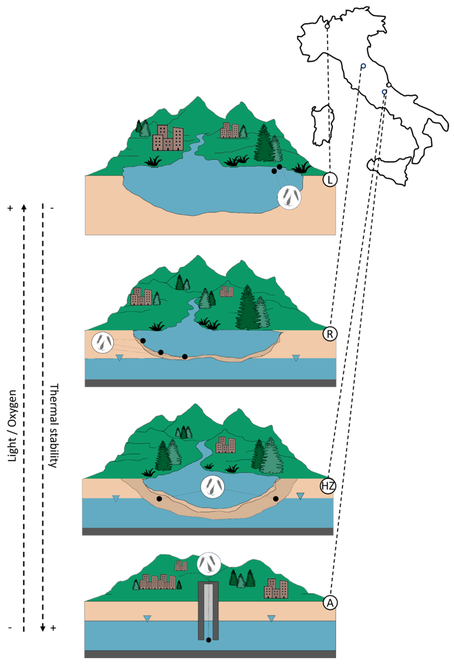

| Light Condition | Temperature Variation | T ± SD (°C) | DO ± SD (mg L−1) | TOC ± SD (mg L−1) | NO3− (mg L−1) | NH4+ (mg L−1) | |
|---|---|---|---|---|---|---|---|
| I A 1 | no light | low | 16.15 ± 1.86 | 4.31 ± 1.76 | 4.79 ± 4.98 | 59.52 ± 42.14 | 0.42 ± 0.14 |
| II HZ 2 | no light | moderate | 9.79 ± 3.70 | 6.09 ± 2.70 | 1.85 ± 0.48 | 3.67 ± 3.02 | 0.64 ± 2.33 |
| R 3 | light | high | 13.05 ± 4.09 | 13.41 ± 0.88 | 1.88 ± 0.11 | 0.16 ± 0.11 | 0.19 ± 0.17 |
| III L 4 | light | high | 23.21 ± 1.96 | >9.00 ± 2.00 | ND | 0.38 ± 0.79 | 0.46 ± 0.79 |
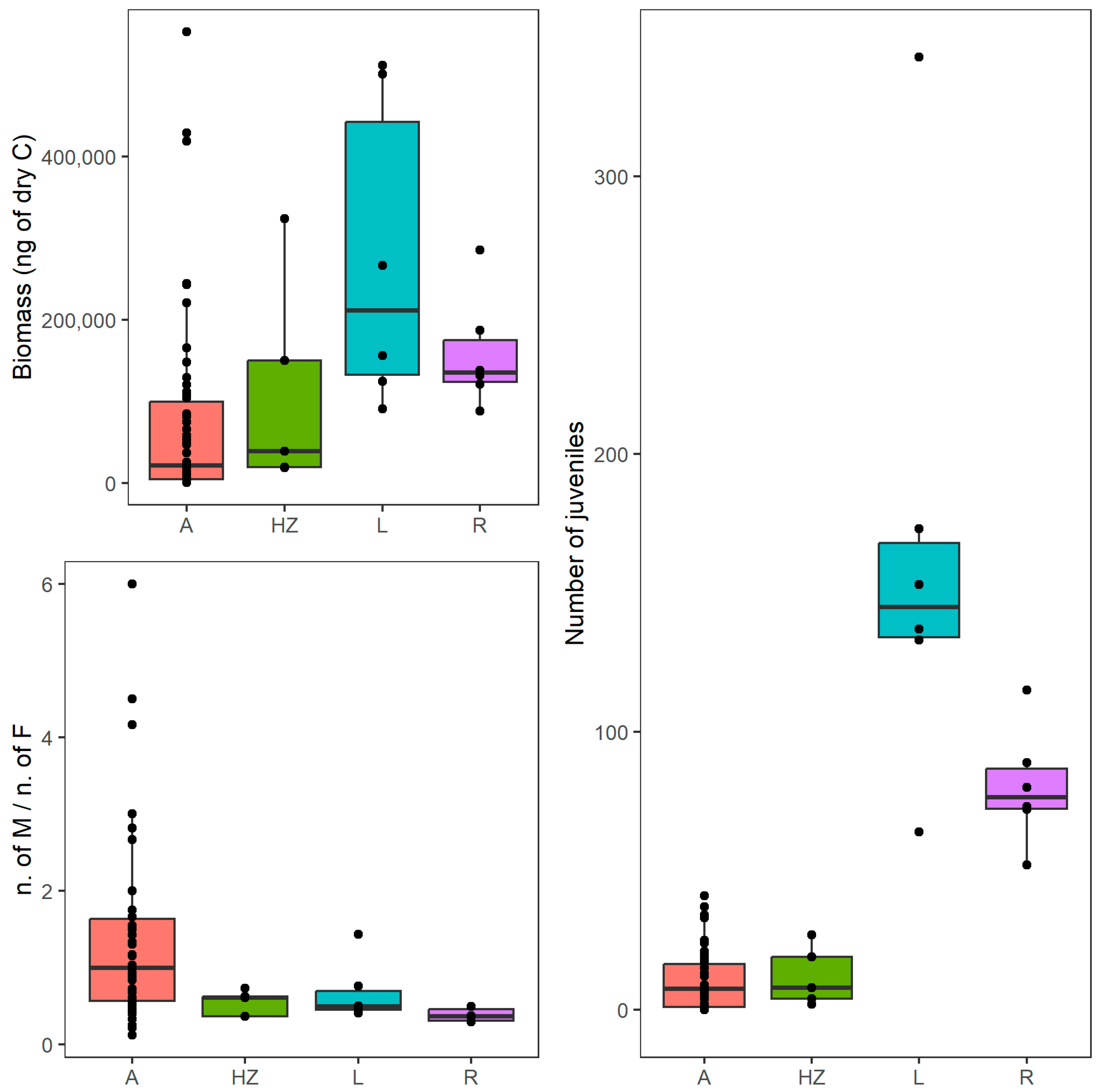
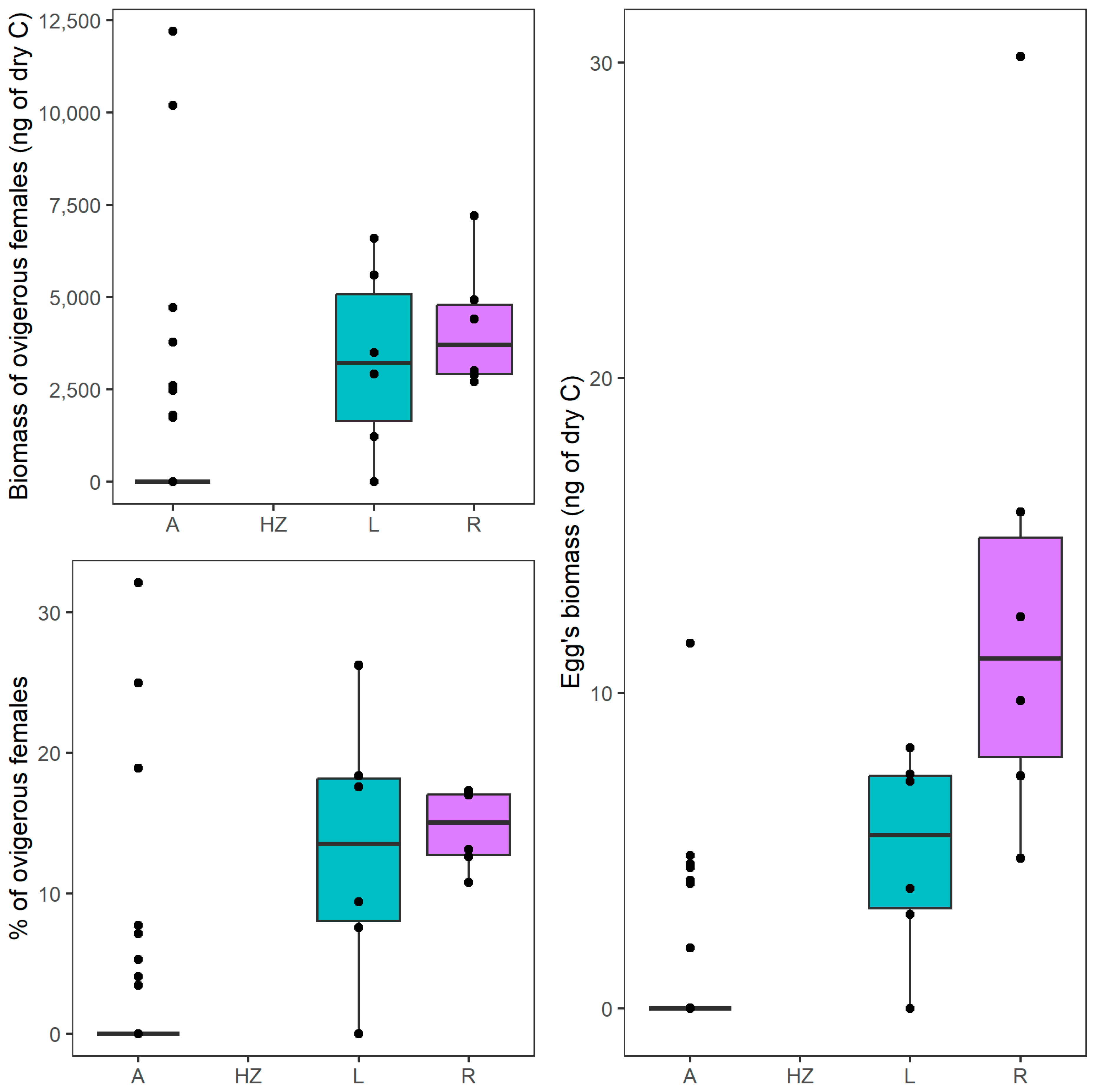
| # | Trait | Habitat | Min | Max | Median ± SD |
|---|---|---|---|---|---|
| 1 | Cumulative biomass | A | 309 | 552,465 | 21,386 ± 115,767 |
| HZ | 18,397 | 323,936 | 38,800 ±131,370 | ||
| R | 87,693 | 285,609 | 134,842 ± 70,012 | ||
| L | 90,750 | 511,377 | 211,249 ± 188,617 | ||
| 2 | Biomass of juveniles | A | 0 | 152,936 | 5661 ± 31,844 |
| HZ | 1044 | 30,387 | 7471 ± 12,105 | ||
| R | 20,576 | 53,136 | 36,965 ± 10,393 | ||
| L | 27,444 | 251,411 | 68,498 ± 82,159 | ||
| 3 | Biomass of ovigerous females | A | 0 | 12,196 | 0 ± 2296 |
| HZ | nd | nd | nd | ||
| R | 2704 | 7199 | 3702 ± 1728 | ||
| L | 0 | 6598 | 3208 ± 2512 | ||
| 4 | Egg biomass | A | 0 | 12 | 0 ± 2 |
| HZ | nd | nd | nd | ||
| R | 5 | 30 | 11 ± 9 | ||
| L | 0 | 8 | 6 ± 3 | ||
| 5 | Body size dimorphism | A | 0.7 | 1.2 | 0.9 ± 0.1 |
| HZ | 0.9 | 1.2 | 0.1 ± 0.1 | ||
| R | 0.9 | 1.0 | 0.9 ± 0.05 | ||
| L | 0.9 | 1.0 | 0.9 ± 0.05 | ||
| 6 | Relative egg size | A | 8 × 10⁻⁷ | 3 × 10⁻³ | 1 × 10⁻³ ± 1 × 10⁻³ |
| HZ | nd | nd | nd | ||
| R | 1 × 10⁻³ | 5 × 10⁻³ | 3 × 10⁻³ ± 1 × 10⁻³ | ||
| L | 1 × 10⁻³ | 2 × 10⁻³ | 2 × 10⁻³ ± 0.4 × 10⁻³ | ||
| 7 | Egg volume (µm3) | A | 278 | 312,898 | 115,007 ± 89,903 |
| HZ | nd | nd | nd | ||
| R | 28,817 | 102,717 | 59,745 ± 25,628 | ||
| L | 35,354 | 80,445 | 46,992 ± 20,905 | ||
| 8 | Number of eggs/sac | A | 2 | 60 | 14 ± 19 |
| HZ | nd | nd | nd | ||
| R | 15 | 15 | 14 ± 1 | ||
| L | 11 | 17 | 15 ± 2 | ||
| 9 | Number of juveniles | A | 0 | 41 | 7 ± 11 |
| HZ | 2 | 27 | 8 ± 11 | ||
| R | 52 | 115 | 76 ± 21 | ||
| L | 64 | 343 | 145 ± 94 | ||
| 10 | Ratio of juvenile/adult abundances | A | 0.2 | 17.0 | 0.6 ± 2.8 |
| HZ | 0.3 | 5.0 | 0.6 ± 2.0 | ||
| R | 0.5 | 0.7 | 0.6 ± 0.1 | ||
| L | 0.4 | 1.7 | 0.9 ± 0.5 | ||
| 11 | Ratio of male/female abundances | A | 0.1 | 6.0 | 1.0 ± 1.2 |
| HZ | 0.4 | 0.7 | 0.6 ± 0.2 | ||
| R | 0.3 | 0.5 | 0.4 ± 0.1 | ||
| L | 0.4 | 1.4 | 0.5 ± 0.4 | ||
| 12 | Percentage of ovigerous females | A | 0.0 | 32.1 | 0.0 ± 31.00 |
| HZ | nd | nd | nd | ||
| R | 10.7 | 17.3 | 15.0 ± 2.8 | ||
| L | 0.0 | 26.3 | 13.5 ± 9.3 |
Disclaimer/Publisher’s Note: The statements, opinions and data contained in all publications are solely those of the individual author(s) and contributor(s) and not of MDPI and/or the editor(s). MDPI and/or the editor(s) disclaim responsibility for any injury to people or property resulting from any ideas, methods, instructions or products referred to in the content. |
© 2023 by the authors. Licensee MDPI, Basel, Switzerland. This article is an open access article distributed under the terms and conditions of the Creative Commons Attribution (CC BY) license (https://creativecommons.org/licenses/by/4.0/).
Share and Cite
Tabilio Di Camillo, A.; Galassi, D.M.P.; Fiasca, B.; Di Cicco, M.; Galmarini, E.; Vaccarelli, I.; Di Lorenzo, T. Variation in Copepod Morphological and Life History Traits along a Vertical Gradient of Freshwater Habitats. Environments 2023, 10, 199. https://doi.org/10.3390/environments10120199
Tabilio Di Camillo A, Galassi DMP, Fiasca B, Di Cicco M, Galmarini E, Vaccarelli I, Di Lorenzo T. Variation in Copepod Morphological and Life History Traits along a Vertical Gradient of Freshwater Habitats. Environments. 2023; 10(12):199. https://doi.org/10.3390/environments10120199
Chicago/Turabian StyleTabilio Di Camillo, Agostina, Diana Maria Paola Galassi, Barbara Fiasca, Mattia Di Cicco, Emma Galmarini, Ilaria Vaccarelli, and Tiziana Di Lorenzo. 2023. "Variation in Copepod Morphological and Life History Traits along a Vertical Gradient of Freshwater Habitats" Environments 10, no. 12: 199. https://doi.org/10.3390/environments10120199
APA StyleTabilio Di Camillo, A., Galassi, D. M. P., Fiasca, B., Di Cicco, M., Galmarini, E., Vaccarelli, I., & Di Lorenzo, T. (2023). Variation in Copepod Morphological and Life History Traits along a Vertical Gradient of Freshwater Habitats. Environments, 10(12), 199. https://doi.org/10.3390/environments10120199