Small Scale Rainfall Partitioning in a European Beech Forest Ecosystem Reveals Heterogeneity of Leaf Area Index and Its Connectivity to Hydro-and Atmosphere

Abstract

(1) Background: Leaf area index (LAI) is an essential structural property of plant canopies and is functionally related to fluxes of energy, water, carbon, and light in ecosystems; coupling the biosphere to the geo-, hydro-, and atmosphere. There is an increasing need for more accurate and traceable measurements among several spatial scales of investigation and modelling. We hypothesize that the spatial variability of LAI at the scale of crown sections of a single European beech (Fagus sylvatica L.) tree in a highly structured, mixed European beech-Norway spruce stand can be determined by simultaneous records of precipitation; (2) Methods: Spatially explicit measurements of throughfall were conducted repeatedly below beech and in forest gaps for rain events in leafed and in leafless periods. Subsequent analysis with a new regression approach resulted in estimating leaf and twig water storage capacities (SC_leaf/twig) at point level independent of within-crown lateral flow mechanisms. Inverse modelling was used to estimate spatial litterfall (n = 99) distribution and litter production (mass, area, numbers) for single trees, as a function of diameter at breast height; (3) Results: As revealed by a linear mixed-effects model, SC_leaf at the center of a beech canopies amounts to 4.9 mm in average and significantly decreases in the direction of the crown edges to an average value of 1.1 mm. Based on diameter-sensitive prediction of litter production, specific leaf area wetting capacity amounts to 0.260 l·m⁻². A linear within-canopy dynamic of LAI was found with a mean of 17.6 m²·m⁻² in the center and 4.0 m²·m⁻² at the edges; and (4) Conclusions: The application of the method provided plausible results and can be extended to further throughfall datasets and tree species. Unravelling the causes and magnitude of spatial- and temporal heterogeneity of forest ecosystem properties contribute to overall progress in geosciences by improving the understanding how the biosphere relates to the hydro- and atmosphere.

1. Introduction

In forest ecosystems, tree individuals modify the abundance and allocation of ecological resources such as water and light due to their spatial and seasonal biomass distribution [1,2,3]. This is reflected by substantial small-scale variation in resource patterns and ecological functioning of forests [4,5]. Thus, forests as parts of the biosphere interact on multiple scales with the hydro- and atmosphere. The partitioning of rainfall into interception loss, stemflow, free throughfall, and canopy throughfall depends on tree species, tree metrics, and vegetation patterns caused by clumping of leaves and the creation of canopy gaps [6]. Transmission, absorption, and reflection of light radiation are largely modified by tree species-specific phenological rhythmic (e.g., foliated vs. leafless periods), as well as the morphologies of leaves and crowns, the angles of leaves and twigs, and by effects on the spatial arrangement of leaves [4,7,8]. For both, the abundance and distribution of water and light, the biomass and area of leaves play pivotal roles and can be expressed for example as leaf area index (LAI), as relevant property of the biosphere.

The LAI is defined as the cumulative one-sided area of leaves per unit stand area and is expressed in m² per m² [9,10]. The same applies for the surface area of woody plant compartments, the woody area index (WAI) and the sum of LAI and WAI, the plant area index (PAI). The LAI affects the distribution and consumption of ecological resources in forest ecosystems and therefore is closely linked to hydrological and atmospherical processes related to the cycles of water-, energy-, and carbon, as well as gas fluxes at higher spatial scales. A variety of ecological processes in the forest and on the forest floor are linked to the resource input at a particular location, among them germination and germinant growth of trees [11,12,13,14], water uptake by plants [5], and organic matter decomposition with subsequent nutrient release by soil microorganisms [15,16,17]. Despite ecological modelling today resolves to the tree or at least cohort (groups of similar trees) level, the small-scale variability of LAI and WAI are not explicitly considered. Research results were commonly reported at the spatial scale of groups of trees or forest stands [18,19]. However, some studies indicated horizontal variability of LAI within the crown of single trees in orchards, olive- and nut plantations, as well as in forest ecosystems for juvenile alder and beech [9,20,21,22,23,24] and strong spatial autocorrelations in point-scale LAI measurements with a range between ten and 15 m, which equals average crown dimensions [25,26].

The application of indirect ground based optical methods such as LAI-2000-series (plant canopy analyzer), TRAC (Tracing Radiation and Architecture of Canopies), digital hemispherical photography, line quantum sensors, imaging instruments, and terrestrial laser scanning that aims to generate estimates of LAI for particular measurement points is partly restricted by the variability and complexity of canopy and stand structures in forests [8,27,28,29]. In particular, in spatially heterogeneous stands with mixed tree species and variable age composition, currently applied methodologies for LAI determination do not provide reliable quantitative estimates on small-scale variability of leaf distribution and subsequent effects on distribution of throughfall water and light radiation.

In contrast to the complex physics of light and subsequent restrictions on applicability of ground-based light radiation measurements [14,27,30], we hypothesize that small-scale (<1 m) measurements of water movement via throughfall in forests provide a reliable, causal and mathematical sound attempt to quantify LAI and WAI at the spatial scale of the respective crown section above the measurement point. In detail, we believe this is in particular the case for the causal relationship between interception loss, as expressed by the respective canopy storage capacity: SC_canopy, and the respective intercepting crown biomass [31,32,33]. In this context it is important to note that the specific wetting capacity (SWC, l·m⁻²) of the single canopy compartment (e.g., leaves, bud, twig) is linearly related to the respective wetted surface area [34]. The sum of all compartments at a given area results in the cumulative storage capacity (SC) [11,35].

As an alternative method for small-scale horizontal LAI quantification, we propose an attempt that is based on exact perpendicular measurements of throughfall below the canopy and the subsequent calculation of SC_canopy, leaf storage capacity (SC_leaf), and twig storage capacity (SC_twig). The general idea is based on previous work [31,33,35,36], however, no attempts still exist for the specific application of fine-scale LAI quantification. The reasons for that are diverse and partly relate to the spatial scale of interest of the studies and the considered hydrological factors:

(1) At the level of the forest stand, the commonly applied calculation approach for the estimation of SC_canopy is based on water balance approaches that integrate over larger spatial scales [6,37] than required for small-scale LAI estimation.

(2) The tree species specific occurrence of stemflow or relative throughfall accumulation at dripping points affect throughfall patterns. Depending on tree species, bark properties, and branch angel; the amount and spatial patterns of lateral flow must be determined using direct or indirect measurement methods (e.g., stemflow or LIDAR observations). In such cases, the additional mathematical consideration of lateral flow is mandatory, but was not included in previous studies [35,36,38,39,40].

(3) Many datasets suffer from the occurrence of strong wind, time dependent evaporation, and spatially variable rainfall events in the course of explicit measurement campaigns. These factors affect applicability of the LAI estimation approach in an unwanted manner.

The proposed approach relies on the methodological differentiation between SC_leaf and SC_twig obtained from throughfall data during foliated and leafless periods in order to separate interception of leaves and twigs. Based on the investigation and quantification of beech leaf mass and area [8,31,32,41,42,43] the relationship between leaf area and SC_leaf can be established. Single tree leaf amount can be derived by inverse modelling [44,45]. This method was established in seed dispersal research [46,47,48] and can be used for spatially explicit modelling of single tree LAI based on SC_leaf.

This study presents an approach to (i) detect and (ii) quantify the variability of leaf distribution within single tree crowns of European beech (Fagus sylvatica L.). Both goals will be achieved by the investigation of the redistribution of gross precipitation by measurements of net precipitation at specific locations underneath beech tree crowns. The observations consider several rainfall events (n = 33) and include foliated and leafless phenological phases. As field-data originate from a mixed stand of European beech and Norway spruce (Picea abies (L.) Karst.), the approach was tested in a highly structured case situation. For European beech, (iii) single tree leaf masses, leaf amounts and leaf areas were predicted by using inverse modelling of litter dispersal based on spatially highly resoluted litter fall measurements. Leaf predictions were compared to associated measurements of SC_leaf at the single-tree level (iv).

2. Materials and Methods

2.1. Study Site

The study site is located in the Tharandt Forest in Saxony, Germany, at an elevation of 360 m a.s.l. at 50°59′ N and 13°30′ E. The climate at these low mountainous elevations is typically moist (800 mm total annual precipitation) with a mean annual temperature of 7.2 °C. A squared study site (0.75 ha) was established within a 111-year-old single-storey mixed stand of European beech and Norway spruce in 2006 (Figure 1) [39]. The mixed stand had not been managed for at least 10 years. The soil is a typical stagnic cambisol with mesotrophic, moderately moist conditions, originating from quartz felsite overlaid by loess loam. Although the total basal area indicates a regular stand density (

Table 1. Characterisation of the studied mixed beech-spruce stand. For more information see [39].

Tree Species	Tree Number (ha−1)	Mean Tree Height (m)	D (cm)				Basal Area (m2·ha−1)	Growth Rate100 (m³·ha−1·a−1) 1	Crown Length (% of Tree Height)
			Mean	SD 2	Max.	Min.			Mean	SD
Beech	139	34.5	44.2	10.8	75.4	21.2	22.8	8.0	66.6	± 9.9
Stand total	227						35.8

¹ Growth rate100, i.e., the average total timber growth normalized to a stand age of 100 years. It is considered as an indicator for overall yield in forest growth research. ² SD standard deviation. D is diameter at breast height. Beech is Fagus sylvatica.

), the spatial heterogeneity of the stand density was high due to the abundance of tree clusters and gaps. The data in the Table 1, indicates a balanced mixture of beech and spruce and typically high crown length for beech.

Beech trees at the study site showed a significant linear correlation of crown radius and diameter at breast height (D) (with a slope of the linear relationship of 10.8 and an intercept of 0, R² = 0.55, p < 0.0001). For further information see [39].

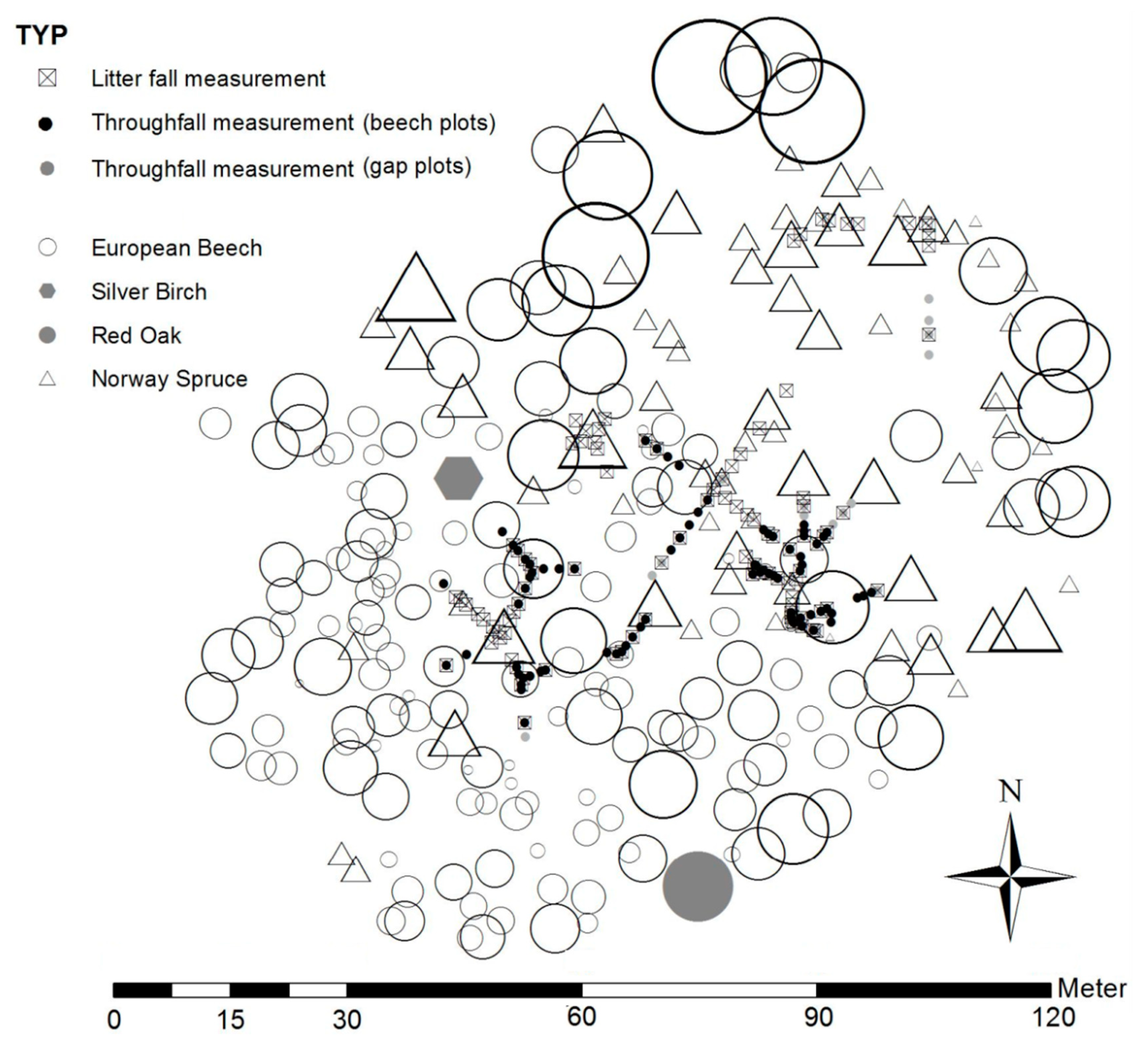
2.2. Field Design for Throughfall and Litter Sampling

Within the study site, 175 measurement points were randomly placed with irregular distance along pre-stratified transects among single trees, i.e., beech-spruce, beech-beech, and spruce-spruce (Figure 1); including small gaps (following [49,50]). Each measurement point was assigned to one out of four cover strata: (i) beech, (ii) spruce, (iii) gap, or (iv) mixed. For each measurement point, the distance from the bole of the nearest dominant tree, i.e., the tree providing vertical crown cover, was recorded. The relative distance (relDist) was calculated as the ratio of the distance to the bole and the crown radius of the respective dominant tree ranging between 0.1 and 1.0 [39,51]. In contrast to the study of [39], in the present account a reduced number of throughfall measurement points were considered (see Section 2.4.1) with n = 76 for beech strata and n = 15 for the gap strata (

Table 2. Sample size (n) in each of the canopy strata. The relative distance for each measurement point underneath beech was calculated as the ratio between the distance to the stem (in m) and the crown radius of the dominant tree (in m) ranging from 0.1 to 1.0, and subsequently classified into deciles.

Canopy Stratum	Sample Size (n) According to Relative Distance Class										Total n
	0–0.1	0.1–0.2	0.2–0.3	0.3–0.4	0.4–0.5	0.5–0.6	0.6–0.7	0.7–0.8	0.8–0.9	0.9–1.0
Beech	5	10	9	6	8	8	8	9	8	5	76
Gap											15

). Detailed analyses of the full data set can be found in [39,52,53].

Overall, 17 beech trees were assigned to the selected throughfall measurement points under beech. The crown radii varied substantially between 2.1 and 6.4 m. The diameter at breast height ranged between 21.2 and 60.3 cm.

In total, 99 out of 175 measurement points were randomly selected for placing the litter fall traps (see Section 2.3.1). Some of the throughfall and litter fall measurement points were taken at the outermost trees of the study plot, but potential edge effects can be ignored due to the 15 m buffer zone around the study site.

2.3. Litter Biomass and Leaf Area

2.3.1. Measurement of Litter Fall

In order to determine the one-year leaf litter fall and leaf dispersal of beech, litter traps were installed randomly at pre-selected measurement points (n = 99). Litter was collected in the period from 19 June 2006 to 18 June 2007. Litter traps were inverted conical mesh traps, with a mesh width of 0.5 mm, designed to catch all leaves at a height of 1.0 m above ground floor in a circular area of 0.2 m² [54]. After clearing the traps at three times during the year (25.10.2006; 01.12.2006; 18.06.2007) the litter was sorted by species and plant compartment by hand, oven dried at 60 °C for 5 days until constant weight [8,15], and subsequently weighted (accuracy of 0.01 g). The leaf litter data obtained for each measurement point were converted into density data per m² and served as input data for leaf dispersal model analysis (see Section 2.3.2).

Leaf mass was obtained from randomly selected litter traps (n = 15, 15% of all litter traps) by selection, counting, drying, and weighing of exactly 250 leaves per trap. Specific leaf area was determined by sampling freshly fallen leaves. Overall, 15 times 100 fresh leaves were collected in autumn 2006 and the leaf area was measured using a LI-3000 Area Meter (LI-COR, inc) with an accuracy of 0.01 cm² [41,55]. Leaf mass and leaf area was used to calculate normalized specific leaf mass (g·leaf⁻¹), normalized leaf area (cm²·leaf⁻¹) as well as specific leaf area (cm²·g⁻¹) [8,23,36,42].

Calculated mean and standard deviation (SD) consider cumulative investigation within sampling units (i.e., litter traps). For statistical analysis we follow [17]. Normality, homogeneity and independence in the litter fall dataset were assessed. All statistical analyses were performed using SPSS (IBM) and R (R version 3.5.1, R Core Team, 2013).

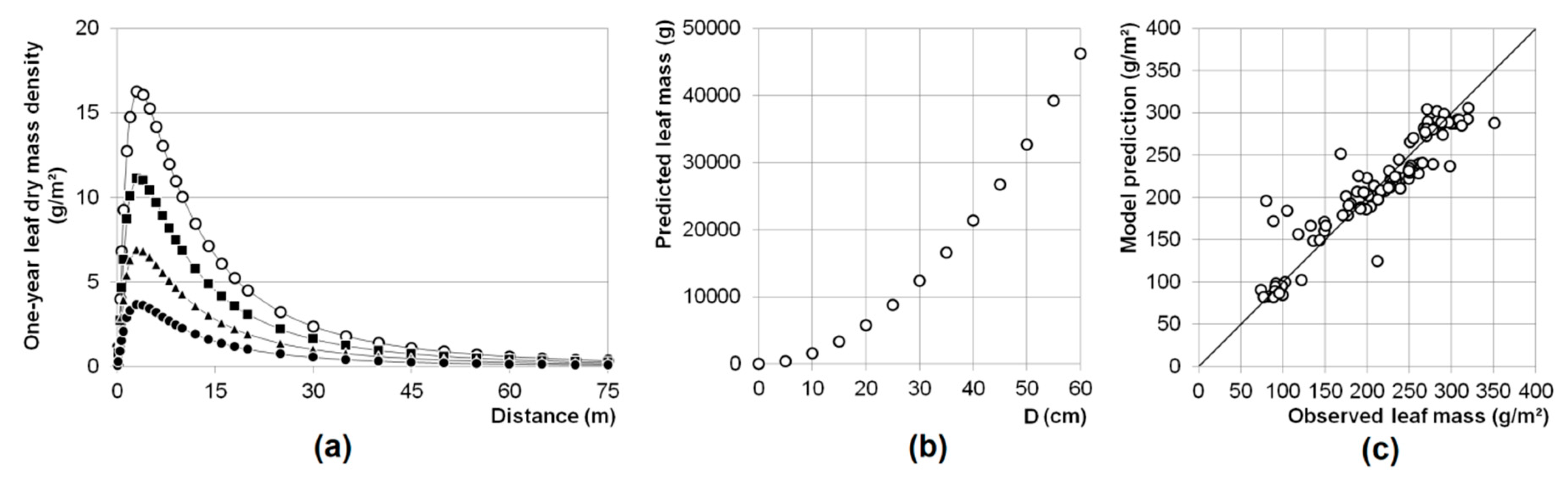
2.3.2. Calculating Leaf Dispersal and One-Year Single Tree Leaf Production

For the prediction of single tree leaf mass, a leaf dispersal model was used according to [56] and the provided R-script. This statistical tool utilizes a phenomenological model and integrates directionality, e.g., in seed dispersal of anemochorous forest trees. Thus, the model can calculate isotropic (same dispersal in all directions) and anisotropic dispersal (unequal spatial distribution due to directed vectors such as wind). Further details on inverse modelling are described in [47,48,54,57,58].

The leaf dispersal model multiplies an estimator of single tree leaf mass by a spatial dispersion kernel [45,56]. One-year leaf mass dispersal of beech was modeled by using the log-normal distribution as density function f of the distance (Dist) (Equation (1)) and combined this with distorted-distance models (not shown), considering anisotropic dispersal [56,59]. The log-normal distribution is defined by parameters δ and μ:

$$f=\frac{e^{-\left(\frac{{\left(\ln Dist-\mu \right)}^2}{2\ast {\delta }^2}\right)}}{2\ast \pi \ast Dis{t}^2\ast \sqrt{2\ast \pi \ast {\delta }^2}}\ast \phi ,\phi =e^{\alpha \ast D^z},$$

(1)

The original version of the model [56] estimates the parameter fecundity φ that represents the leaf mass produced (g) by a single beech tree with a respective diameter at breast height (mm), and parameter α that weights the allometric relationship between φ and D. In Equation (1), we modified the aforementioned term by replacing the former quadratic exponent for D by a free varying exponent (z). In consequence, D, α, and z allow for the estimation of total leaf mass of single beech trees (i.e., φ) in mixed forest stands. In other words, single tree leaf mass can be calculated based on modelled leaf litter dispersion.

The mean D of beech at the study site was 44.2 cm, therefore, we focus the model output for an average tree with a D 45.0 cm and for the total D-range of 15 to 60 cm. For directionality in leaf dispersal [44,60], the distance (Dist) may be distorted [59,61]. According to [56], additional parameters for the assumption of an anisotropic dispersal in the form of an elliptic distorted-distance model can be estimated within the inverse model: coherency β, drift γ, and rotation angle ψ. In consequence, the model that considers anisotropy simultaneously approximates six parameters. In order to account for the number of model parameters and thus model complexity, Akaike’s information criterion (AIC) and the log likelihood estimate were used to evaluate model performance together with analysis of correlation between observed and predicted values. This attempt aims to find the model that includes most information and best describes the data [45].

Whether an isotropic or a much more complex anisotropic model fits the data better was tested by a Bootstrap-approach. The basic idea of any sort of hypothesis test is to compare the observed value of a test statistic with the distribution that it would follow if the null hypothesis were true. The null is then rejected if the observed value is sufficiently extreme relative to this distribution [62]. We considered isotropic and anisotropic models as being nested. Thus, to test for significant differences between isotropic and anisotropic models we constructed an empirical sampling distribution. Therefore, we adopted a parametric bootstrap approach based on the likelihood ratio statistic [63,64], The test statistic is: 2(loglike_non-isotrop–loglike_isotrop).

The null-hypotheses states that both models, isotropic and anisotropic, fit the observed leave-amount of litter trap data equally well. The samples created by the bootstrap data generating process should not just reflect the null hypothesis [65]; but it is recommended, that the bootstrap samples even satisfy the null hypothesis [62]. We assume the leave-amount of litter trap data to be negative binomially distributed (see [56]). We estimated the ‘size’ parameter of a negative binomial distribution to best fit the real data in advance of bootstrapping (library ‘VGAM’ in R [66]). Then, we performed parametric resampling from the data set built from the isotropic model, randomized by the ‘size’ parameter of a negative binomial distribution. Both models, the isotropic and the anisotropic, were fit to each of the 99 simulated data sets.

2.4. Gross Precipitation and Throughfall

2.4.1. Measurement of Gross Precipitation and Throughfall

Measurements were performed in the foliated period from 15 May 2006 to 01 September 2006 when the beech crowns were completely foliated as evaluated by phenological observation and litterfall measurements in the forest stand. Measurements in the leafless period were performed between 20 November 2006 and 15 April 2007. Measurements have taken place in frost-free periods ((i) 20 November 2006 to 15 December 2006, (ii) 03 to 19 January 2007, (iii) 24 February 2007 to 18 March 2007, (iv) 29 March 2007 to 15 April 2007) with no events of snow included in the dataset (see Section 2.4.2).

At all measurement points, data were recorded manually immediately after each single rainfall event [39]. Each recording time was about half an hour. A “single precipitation event” was defined as a period of precipitation preceded by at least four hours of no rain (see [2,32,36]). This defined period allowed for crown drip to be recorded after rainfall, yet was still sufficiently short to prevent evaporation loss from the throughfall collectors [3,67]. If rainfall began again within four hours after the last precipitation, only one rainfall event with a break of less than 4 h was recorded. Precipitation during the night was immediately measured the following morning. Dew and fog precipitation were negligible during our measurement campaigns.

Gross precipitation was determined using five identical funnels installed in an adjacent open meadow (150 m apart). Throughfall was collected at selected measurement points in funnels (area 50 cm²), with a maximum volume of 60 mm of precipitation. Funnels were securely installed in vertical PVC pipes 1 m above ground. Evaporation loss after a rainfall event and before the next measurement was zero because the funnels were inserted into the shaded upper ends of tubes [14,39]. For measurement points with both, throughfall and litter fall measurements throughfall, funnels were placed in very close vicinity of the litter fall trap.

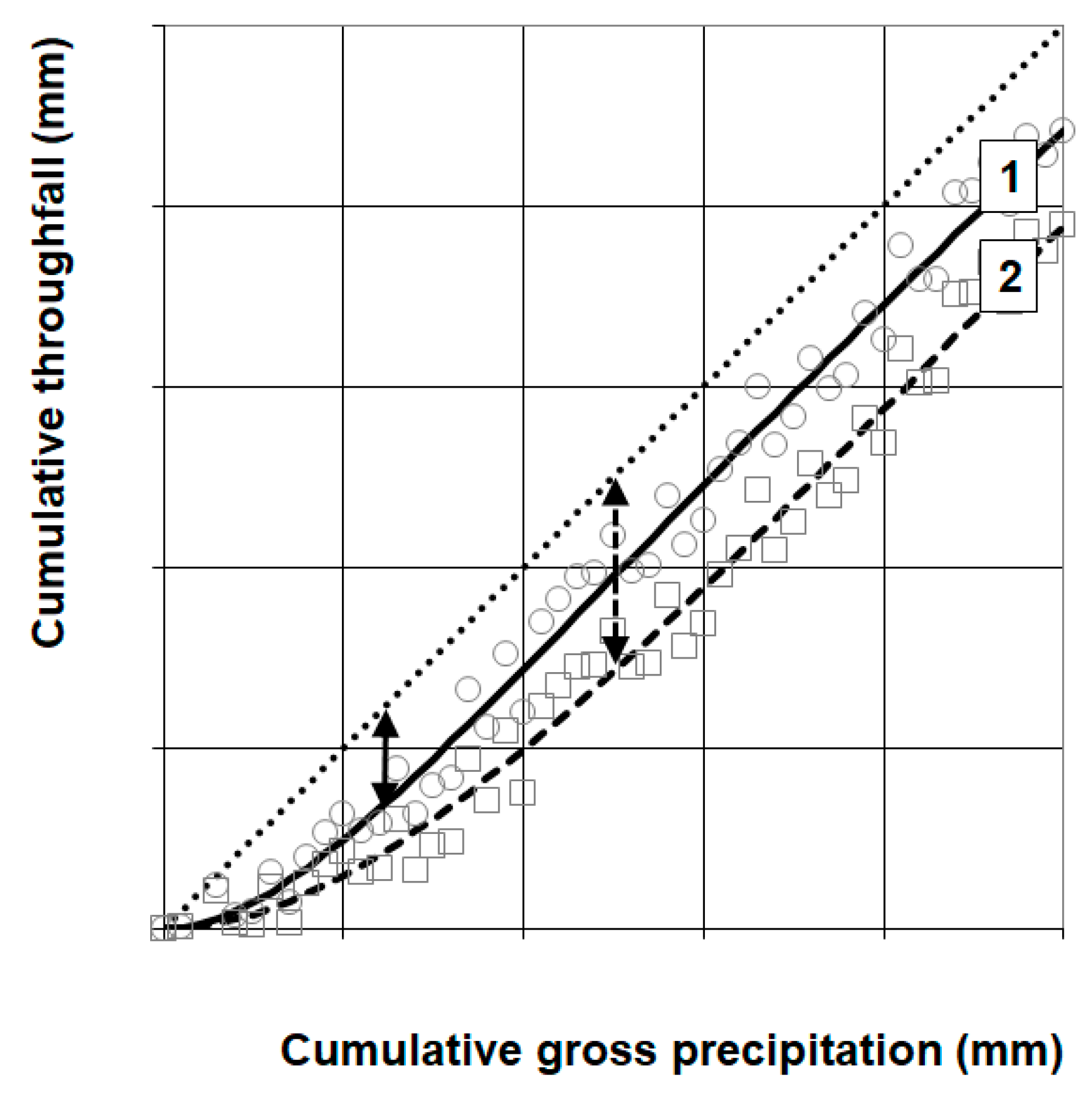
2.4.2. Throughfall Data Inspection and Selection

A meteorological station located at a distance of 500 m from the study site provided reference data for wind speed and dates of rain events. Meteorological data from this station, gross precipitation reference data from the open adjacent meadow, and descriptive statistics of gap throughfall measurements were used for data mining. Data were selected based on a checklist of defined threshold values [39]. Briefly, data-series of single rain events were only included in the following analyses if they (i) were not snow events, (ii) originated from clearly defined single rain events (see definition above), (iii) were not affected by high wind speed intervals during the rain (always average wind speed of 10-min recording interval ≤6 m·s⁻¹), (iv) coincided with simultaneous, almost identical readings from the five reference funnels in the adjacent open meadow, i.e., if the variation coefficient was less than 6%, and (v) data was consistent at measurement points in large gaps and in the meadow, thus indicating homogeneous rain events on a large spatial scale. In sum, during the foliated period 26 out of 36 observed single rain events (intensity range 0.1 to 18.1 mm·h⁻¹) completely fulfilled the requirements mentioned above, amounting to a total precipitation of 208.9 mm. Out of the 26 rain events, 14 yielded less than 5 mm, 5 yielded up to 10 mm, and 7 yielded more than 10 mm, with a maximum gross precipitation of 49 mm. During the leafless period only 7 out of 13 rain events (intensity range 0.1–2.0 mm·h⁻¹) fulfilled the requirements mainly due to the abundance of high wind speeds, amounting to a sum precipitation of 28.5 mm. 3 events yielded less than 5 mm, the other 4 events yielded up to a maximum gross precipitation of 7 mm.

2.5. Storage Capacity of Tree Biomass Compartments

2.5.1. Estimation of Canopy Storage Capacity, Leaf Storage Capacity, and Twig Storage Capacity

Several procedures have been developed to generalise the dynamics of precipitation and throughfall in forests. Commonly, repeated measures at defined measurement fields inside and outside the forest or above the forest were utilised to parameterise equations [68,69,70,71]. According to [39], the nonlinear relationship between gross precipitation and below-canopy throughfall can be represented in a diagram (Figure 2) and lateral water translocation can be taken into account. These diagrams can be applied to data at the spatial level of single measuring points within a stand [26,39]. In general, gross precipitation determines the amount of throughfall, but the specific pattern of this influence depends on the particular position of a given measurement point. In large gaps, throughfall is identical to gross precipitation. Within forest stands, however, interception loss—especially SC_canopy and time-dependent gradual evaporation of intercepted water—leads to a difference between gross precipitation and throughfall at the respective spatial scale. This difference increases with increasing gross precipitation until the SC_canopy is reached. If the gross precipitation is higher than the precipitation needed to saturate the SC_canopy, the slope of the relationship between throughfall and gross precipitation remains constant, if evaporation can be excluded. In this study, the influence of evaporation was minimised (see Section 2.4) and can be neglected in the following theoretical considerations.

In the absence of evaporation, the slope of the relationship between throughfall and gross precipitation should remain constant at the value of one. However, slopes with a value smaller or bigger than one were frequently observed. This observation can only be explained by lateral water translocation within the canopy, indicating lateral discharge or lateral inflow processes within the canopy of a single tree (for beech and Norway spruce see [39]). Although lateral inflow or discharge are either equalised at larger spatial scales or become part of canopy drip or of stemflow, a considerable water deficit or surplus may be created at the plot specific scale. Large variation in SC_canopy might be caused by specific LAI at the measurement point independently of lateral water translocation [51,72]. This can be assessed by diagrams of the relationship between gross precipitation and throughfall of the foliated and leafless period. Finally, the quantification of the differences in SC_canopy between both periods will provide estimates of SC_leaf and SC_twig.

To capture the expected multiple variability in throughfall patterns, we analysed scatterplots of throughfall and gross precipitation. Equation (2) was parameterised by applying nonlinear regression analysis (bootstrap estimator of the standard error using SPSS IBM Inc.) separately (foliated and leafless period) at each measurement point.

$$T=b\ast P\ast \left(1-e^{-\left(\frac{1}{a}\ast P\right)}\right),$$

(2)

where P (mm) represents gross precipitation, T (mm) throughfall, and a and b are parameters. Equation (2) represents the gradual saturation of SC_canopy during small gross precipitation amounts assuming an exponential behaviour. Amounts of gross precipitation exceeding the value of parameter a result in a nearly linear relationship with individual slope parameters for each scatterplot. Equation (2) thus allows for the consideration of the specific threshold in the relationship of gross precipitation and throughfall at each measurement point. In contrast, other studies generally applied an assumed constant threshold for the amount of gross precipitation above which linear behaviour was to be parameterised for the entire study site.

Parameter a determines the gross precipitation amount needed to saturate SC_canopy (mm) at the spatial scale of a single measurement point (Equation (3)). The calculated SC_canopy value at a particular measurement point and in the foliated period equals the sum of SC_leaf and SC_twig. The SC_canopy value at the same point but within the leafless period represents only the SC_twig.

$$SC=P-T,\mathrm{if}\mathrm{P}=\mathrm{a},$$

(3)

2.5.2. Spatial Analysis of Leaf Storage Capacity

A linear mixed-effects model (lme fit by REML, R software, version 3.5.1, R Development Core Team, 2018 [66]) was applied in order to investigate the linear relationship between SC_leaf and relDist (i.e., position below the canopy relative to tree bole or crown edge). To account for nested sampling, tree identity was selected as random factor. However, as spatial correlation at within-group level still occurred, a linear correlation structure was used to model the spatial correlation in these data [73]. As a pattern of heteroscedasticity was observed for the within-group residuals, an exponential variance function structure was used to model heteroscedasticity in the response variable.

The linear mixed-effects model was applied on a balanced subsample (n = 45) of the original dataset in order to account for unequal abundances of measurement points below studied trees. Briefly, a true random number generator (www.random.org) was used to select SC_leaf data of four measurement points in cases of more than four observations per tree.

3. Results

3.1. Leaf Mass

Observed one-year leaf mass per area of beeches ranged from 74.5 to 351.2 g·m⁻² (dry mass; min-max) with a mean of 216.7 g·m⁻² and a SD of 70.5 g·m⁻² (

Table 3. Mean and standard deviation (SD) of leaf litter mass and other leaf properties of European beech in a 110-year old mixed stand.

Variable	Unit	n	Mean	SD
Observed one-year leaf dry mass per area	(g·m−2)	99	216.7	70.5
Leaf mass	(g·leaf−1)	15 × 250	0.0799	0.0040
Leaf area	(cm2·leaf−1)	15 × 100	20.467	2.564
Specific leaf area	(m2·kg−1)		25.616

). Spatially distinct distribution of beech trees (Figure 1), led to high variation of leaf mass distribution within the study site (Kruskal-Wallis-test, p < 0.001). In order to account for spatial clustering of beech trees, the south-west part of the study site showed highest leaf litter masses per area (≥300 g·m⁻²) while lowest values were observed in the spruce-dominated north-east (≤100 g·m⁻²).

Small-scale LAI values can be derived by multiplication of measured leaf masses with calculated leaf mass-area relationships, as a first but simplified approach (see Table 3). LAI values within the observed mixed beech-spruce stand range between 1.9 (min) and 9.0 m²·m⁻² (max) with a mean of 5.6 m²·m⁻² and a SD of 1.8 m²·m⁻². However, these LAI values do not represent estimates for the crown section directly perpendicular to the measurement point since they do not consider the spatial distribution of litterfall, e.g., by wind. The average one-year leaf biomass production in the mixed beech-spruce stand is 2.17 tha⁻¹ (+/−0.70 tha⁻¹ SD). Calculated for a theoretical pure beech stand, one-year leaf biomass production is 3.60 tha⁻¹. The average beech tree with a diameter at breast height of 44.2 cm within the observed mixed beech-spruce stand produced approx. 15.60 kg leaf biomass. In contrast, applying the leaf dispersal model yielded in higher leaf mass production (26.78 kg) of the reference tree (D = 45 cm). The fecundity-parameter α is −1.412, with a value of 1.9 the exponent z is close to two (Figure 3). Based on the AIC and the results of the bootstrapping, the isotropic assumption of leaf dispersion appears to be the superior to the anisotropic model (

Table 4. Statistical comparison of isotropic and anisotropic leaf dispersal model. Model and parametrization according to [56].

Model	Clumping κ	Fecundity α	Fecundity z	Expected Value μ	Variance δ	Coherency β	Bootstrap 1
iso-tropic	10.67	−1.41	1.9	3.72	1.23		P = 0.354
aniso-tropic	10.67	−0.98	1.9	4.42	1.43	0.52
Model	Driftγ	Rotationψ	AIC	Loglike	r	p-Value	Bootstrap 1
iso-tropic			1036.3	−515.2	0.935	<2.2 × 10−16	P = 0.354
aniso-tropic	0.62	2.67	1039.5	−513.7	0.938	<2.2 × 10−16

¹ Bootstrap statistics indicates that anisotropic model does not perform better than the isotropic model. Results were obtained by each of the 99 runs.

). Parameter of the isotropic model were estimated with μ = 3.717 and δ = 1.234. The correlation between observed and predicted values was strong (r = 0.935). The isotropic dispersal model estimated the maximum leaf mass at a distance to the bole of the respective reference tree of 9.0 m (Figure 3a).

Average beech leaf mass amounts to 0.0799 g·leaf⁻¹ with a SD of 0.004 g·leaf⁻¹. Average beech leaf area showed a mean of 20.467 cm²·leaf⁻¹ with a SD of 2.564 cm²·leaf⁻¹ (Table 3). Specific leaf area of beech amounts to 25.61 m²·kg⁻¹. Based on these data, a total number of approx. 335,000 leaves and a total cumulative leaf area of 686 m² were calculated for the reference tree (D = 45.0 cm). Applying measured specific leaf area and the allometric relationship of φ in Equation (1) allowed for the calculation of total leaf area A (m²) of beech trees of various values of D (mm) (Equation (4)).

$$A=25.61\ast \phi =25.61\ast e^{\alpha \ast D^z},$$

(4)

For the stand-specific D-range of 15–60 cm, total leaf area range between 85–1184 m² (

Table 5. Predictions of crown radius, crown area and leaf area and respective approximations of twig and leaf storage capacities (SC_twig, SC_leaf) based on tree D using Equations (5) and (6).

D	Crown Radius	Crown Area	Leaf Area	SCtwig1	SCleaf
(cm)	(m)	(m2)	(m2)	(l·tree−1)	(l·tree−1)
15	1.62	8.2	85.1	3.6	19.6
20	2.16	14.7	146.9	6.3	34.8
25	2.70	22.9	224.5	9.9	54.4
30	3.24	33.0	317.5	14.2	78.3
35	3.78	44.9	425.5	19.3	106.6
40	4.32	58.6	548.4	25.3	139.2
45	4.86	74.2	685.9	32.0	176.1
50	5.40	91.6	838.0	39.5	217.4
55	5.94	110.8	1 004.3	47.8	263.1
60	6.48	131.9	1 184.9	56.9	313.1

¹ Note, twig storage capacity was calculated by distance (relative distance of measurement point to tree bole) independent average value.

). Based on the empirical diameter–crown radius relationship for circular crown projection areas, simple average LAI values for single tree crowns were calculated and ranged between 9.0 and 10.3 m²·m⁻².

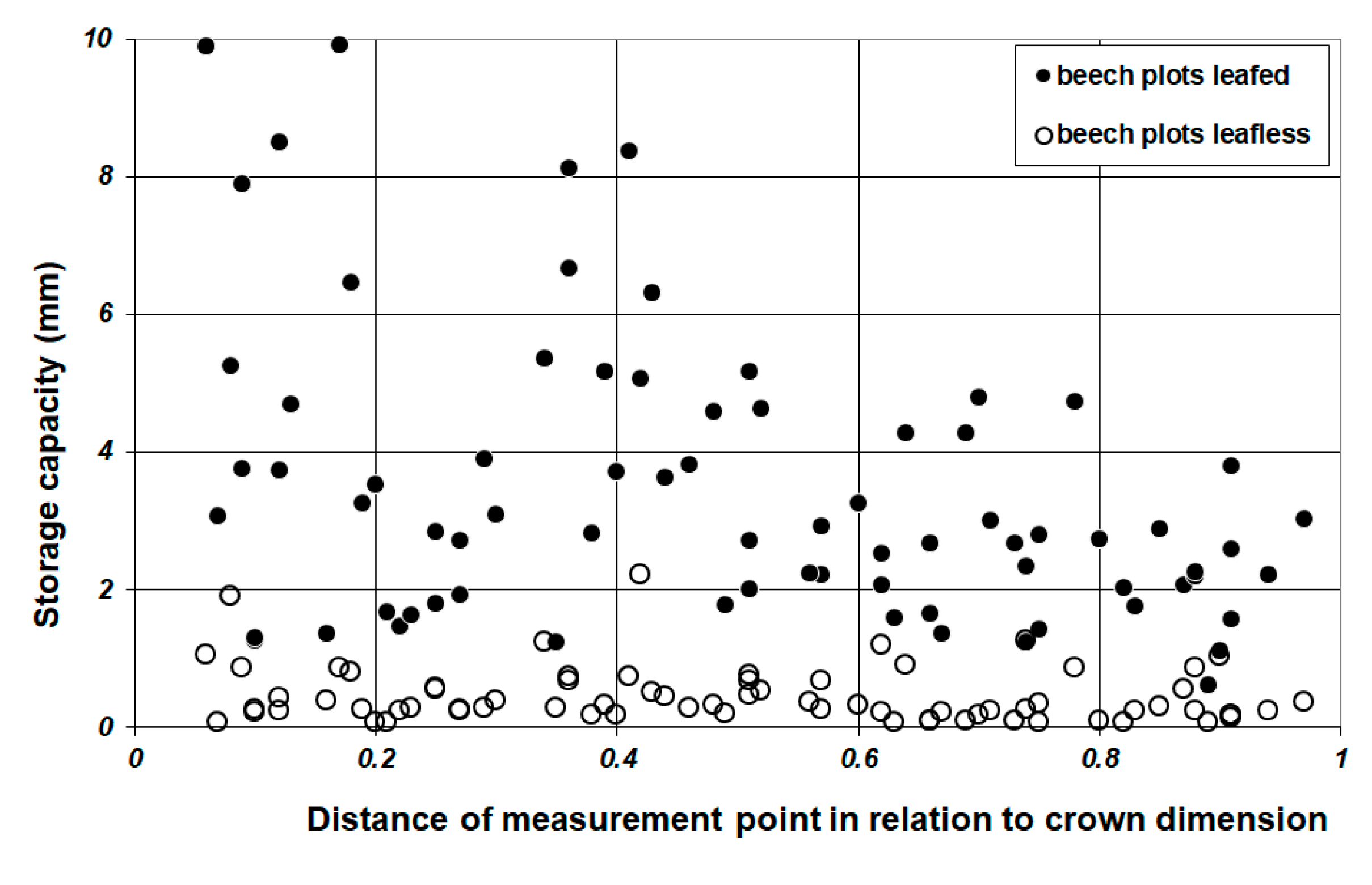
3.2. Throughfall and Storage Capacity

Total gross precipitation of 208.9 mm (foliated period) and 28.5 mm (leafless period) yielded in an average cumulated throughfall of 132.2 mm (63.3% of gross precipitation) and 178.0 (85.2%) in the foliated period and 18.6 mm (65.3%) and 23.4 (82.1%) in the leafless period under beech canopies and in gaps, respectively. Univariate GLM analysis that accounts for the effect of gross precipitation showed a significant effect of phenological phase on throughfall amounts under beech canopies (p ≤ 0.05). However, these small-scale throughfall measurements cannot replace commonly calculated water balance approaches that integrate over larger spatial scales including stemflow for calculating interception. Indeed, it is not the aim of this study to derive representative interception values for the purpose of inter-periodic comparison. Assuming that the sampling design was representative for the entire stand, the canopy cover-specific SC_canopy can be derived by applying Equation (2) for both phenological phases (Figure 4). As expected, SC in gaps calculated from Equation (2) was often 0. As individual measurements in the stand also took place in very small gaps, in the foliated period the overall a value and SC_canopy for the gaps amounted to 0.9 mm and <0.4 mm, respectively (R² = 0.974). In the leafless period the overall a value and SC_canopy for gaps amounted to 0.1 mm and 0.05 mm (R² = 0.913), respectively. Below beech canopies, a gross precipitation (a) of approx. 5.75 mm was needed to reach SC_canopy of approx. 3.0 mm during the foliated period (R² = 0.911) while in leafless period (R² = 0.795) an a value of 0.53 mm and a SC_canopy amount of 0.3 mm were approximated (Figure 4).

The parameterisation of Equation (2) for each individual measurement point was robust for measured data obtained during the foliated period, i.e., always yielded a coefficient of determination larger than 0.950. In contrast, coefficients of determination calculated for data obtained during leafless period varied to a higher degree with the minimum of R² = 0.736 and an average R² of 0.935. 22% of all measurement points have values of R² ≤ 0.900 for the leafless period.

Point specific storage capacities under leafless beech crowns (SC_twig) differed between 0.06–2.21 mm and were independent of the location below the beech canopies (Figure 5). Average SC_canopy of leafless beech crown sectors (SC_twig) amounts to 0.44 mm (+/−0.41 mm SD). Average SC_canopy for measurement points below foliated beech crowns amounts to 3.43 mm (+/−2.09 mm SD) with a minimum of 0.6 mm and a maximum of 9.9 mm. SC_canopy decreases with increasing relative distance to the tree bole (p = 0.000). The relatively high values for SC_canopy (≥6.0 mm) were all located at the inner part of the crown with relative distances below 0.43. The difference between SC_canopy and SC_twig provides an estimate of respective SC_leaf. For beech, mean SC_leaf amounts to 2.9 mm (+/−1.9 mm SD) with a minimum of 0.0 and a maximum of 9.0 mm. The linear mixed-effects model revealed a significant decrease (p = 0.000, R² = 0.828, AIC = 156.8, Equation (5)) in SC_leaf on a balanced subsample (n = 45) from the inner part of the crown near the bole (SC_leaf: mean = 4.89 mm +/−0.59 SD) towards the crown edge (SC_leaf: mean = 1.11 mm +/−0.73 SD).

$$S{C}_{leaf}=3.779\ast relDist+4.893,$$

(5)

3.3. Leaf Area Index (LAI)

Based on diameter-specific calculated crown radii (factor 10.8, see Section 2.1), the total SC_leaf of circular beech crowns with defined values for D can be calculated by integral calculation (Equation (6)). Briefly, computation of the total amount of SC_leaf of a single tree was performed by converting the intensity of SC_leaf (l·m⁻²) to an amount (l) over the entire crown circle and integrating this amount over the distance underneath the crown d(r) from crown centre (0) up to crowns peripheral (r_max) simultaneously. This was done according to [54,57].

$$\begin{array}{c}{\displaystyle {\int }_0^{r_{\max }}\left[S{C}_{leaf}\ast 2\ast \pi \ast r\right]d(r)=}\\ {\displaystyle {\int }_0^{r_{\max }}\left[\left(-3.779\ast relDist+4.893\right)\ast 2\ast \pi \ast r\right]d(r)=}\\ {\displaystyle {\int }_0^{r_{\max }}\left[\left(-3.779\ast \frac{r}{r_{\max }}+4.893\right)\ast 2\ast \pi \ast r\right]d(r)=}\\ {\displaystyle {\int }_0^{\left(\frac{D\ast 10.8}{100}\right)}\left[\left(-3.779\ast \frac{r}{\left(\frac{D\ast 10.8}{100}\right)}+4.893\right)\ast 2\ast \pi \ast r\right]d(r)},\end{array}$$

(6)

For comparison, Table 5 presents the calculated SC_twig and SC_leaf of single beech trees over the D range of 15 to 60 cm. With increasing D, the absolute increase in SC_twig is relatively moderate (3.5 to 56.9 l·tree⁻¹). SC_leaf increases with increasing D with an exponent of 1.4 resulting in absolute values ranging between 19.6 and 313.1 l·tree⁻¹. The relationship between SC_leaf and the total leaf area of the respective beech (Equation (4)) is strongly linear (p = 0.000, R²_korr. = 0.999) with an intercept not significant different from zero. The slope of this relationship represents the specific leaf area wetting capacity for the beech trees within the D range (15–60 cm) and yields a mean value of 0.260 (+/−0.002 SD) l·m⁻² leaf area. The specific leaf mass wetting capacity amounts to a value of 6.656 l·kg⁻¹ leaf mass (+/−0.044 l·kg⁻¹ leaf mass SD) and the specific leaf number wetting capacity amounts to 0.532 lthousand leaves⁻¹ (+/−0.004 l·thousand leaves⁻¹ SD) (

Table 6. Calculated specific wetting capacities for different beech leaf metrics.

Type of Specific Wetting Capacity	Unit	Mean	SD
for leaf mass	(l·kg−1)	6.656	0.044
for leaf area	(l·m−2)	0.260	0.002
for leaf number	(l 1000 leaves−1)	0.532	0.004

).

Figure 6 shows the spatial distribution of point specific LAI values below the beech canopies. LAI values were calculated based on SC_leaf values divided by specific leaf area wetting capacity (Table 6). Predicted crown sector LAI values range between 0.0 and 34.8 m²·m⁻², with an average of 11.2 m²·m⁻² (+/−7.3 m²·m⁻² SD). Highest LAI values of ≥30.0 m²·m⁻² occurred sporadic with no exception in the inner part of the crown near the tree bole (relDist < 0.17). At the crown edge (relDist ≥ 0.9), LAI values amount on average to 7.8 m²·m⁻². In accordance with Equation (5), average LAI (dashed line, Figure 6) significantly decreased with increasing distance to the tree bole (p = 0.000) for the balanced-selected dataset and the linear mixed-effects model with high values in the inner part of the crown (18.8 m²·m⁻²) and low values at the crown edge (4.3 m²·m⁻²).

4. Discussion

4.1. Leaf Area Index (LAI) Estimation

Phytometric research on the spatial distribution of biomass compartments in forest ecosystems are increasingly recognised since the study of [74]. For this research area, most methods rely on laws of the transmission of light radiation on plant tissue surfaces [23,28,55,75]. Alternatively, other methods use litter fall investigations [8,42]. Given its importance, LAI is a common result derived from a number of active and passive remote sensing instruments (satellite or space borne, airborne, and ground based) and modern terrestrial laser scanning applications such as LIDAR [14,29,76,77,78]. For decades, there is a shift in the scale of interest of such studies from the catchment scale to smaller than tree spatial units within heterogeneous forest ecosystems. However, the applicability of indirect optical techniques in more complex forest ecosystems is critically questioned. Therefore, direct methods [20,79,80] and 3-D-modeling approaches that rely on simplified assumptions on the geometry of tree crowns and that are hardly to validate dominated the research on spatial distribution of single tree compartments [4,9,14,18,76,81,82,83,84,85,86]. Results point to tree individual and stand-specific horizontal and vertical variability of biomass compartment distribution with a diverse mixture of zones of no or low and of high biomass as the common situation [20,24,87,88,89,90]. The simultaneous occurrence but variable signal of LAI and WAI restrict spatial analyses of canopy properties on forest ecosystems characterized by foliated and leafless periods and respective repeated measures among these phenological phases [24,29,32,70,91].

In the present account, we found strong indications of horizontally variable LAI`s within the canopy of single trees confirming the results of studies by [20,21,22,23]. Mottus, M. et al. [9] reported LAI’s of 5 within the crown center of juvenile alder trees with a rapid decrease towards crown edges. The observed small-scale LAI distribution as obtained by our approach using throughfall measurements resampled the spatial below-canopy gradients of [9] but LAI values are in general at a higher level. In our study, the spatial gradients were also indicated by simple litter fall measurements. Only a few studies that investigated LAI’s for mature beech trees are available. For example, [24] found average LAI between 2.3 and 3.5 m²·m⁻² with a coefficient of variation between 7 and 24%. The authors concluded that “tree-to-patch centre distance” was an important determinant for LAI distribution at the grid-scale (10-m spacing) with the closer the measurement point to the tree bole the higher the LAI. The same applies for other common species such as Scots pine and oak. Comparable estimates of LAI for pure beech stands were reported in [18] with LAI between 7 and 9 m²·m⁻², in [92] with a LAI of 6.4 in non-fruiting years and 4.5 fruiting years, in [19] with 6, in [43] with an average LAI of 7.4 (minimum: 5.6, maximum: 9.5) as well as in [93] with LAI of 5.6. Depending on spatial stand structure, Ahrends, B. et al. [94] reported LAI values in the range of 0 to 12 while [3] reported values between 5.8–13.3 m²·m⁻². Konôpka, B. et al. [42] reported a LAI value of 14.9 m²·m⁻² for juvenile beech stands. One common feature of the above-mentioned studies is that they do not explicitly included tree-stem or crown edge distance as factor on horizontal canopy LAI distribution. We included such spatial dependencies and observed maximum values of LAI ≥30 in close vicinity to the tree bole. The more or less vertical arrangement, branching pattern, and accumulation of twigs in the top of the crown may contribute to this spatial accumulation of leaves, and leaf areas respectively. Our analysis shows that close to stem LAI can be spatially very variable. Despite this variability, the mean LAI is higher in the crown center of beech trees than at the crown periphery. This might represent a general rule in crown architecture of Fagus sylvatica and might contribute to the overall eco-physiological strategy of this tree species.

4.2. Leaf Mass Prediction, Leaf Ratio Determination, and Leaf Dispersion

Crucial factors for LAI modelling are reliable estimates of leaf masses and the subsequent calculation of leaf areas based on specific leaf area. The variability of annual leaf production is high depending on correlated factors such as carbohydrate formation and allocation, seed production, and forest disturbances in the consequence of abiotic and biotic impacts. Vertical leaf size plasticity in response to light availability is well known for European beech [19,42]. For the present account, leaf plasticity in beech crowns is indicated by large standard deviations of specific leaf area ratios, despite large sample size for leaf dispersal (n = 99) and leaf ratio determination (15 × 100−250 leaves) compared to other studies (see for example [32]). Konôpka, B. et al. [42] reported comparable estimates of specific leaf area of juvenile beech trees (27.3 m²·kg⁻¹) based on sampling of approx. 1000 leaves originated from various crown sectors and among tree individuals of different social positions (dominant vs. subordinated) of the forest stand. Within the class of dominant trees, specific leaf area reached values of 20 m²·kg⁻¹ while subordinated trees showed significantly higher values (~45 m²·kg⁻¹). These variable ranges were confirmed by the literature: Leuschner, C. et al. [43] reported specific leaf areas between 19 and 24 m²·kg⁻¹, Grote, R. et al. [19] reported values between 10 and 40 m²·kg⁻¹, Dyderski, M. et al. [95] found 35 m²·kg⁻¹ for beech seedlings and saplings, Forrester, D. et al. [96] reported a value of 21.5 ± 5 m²·kg⁻¹ derived from several studies of trees older than 50 years which matches the value of 21.3 m²·kg⁻¹ reported by [94]. Forrester, D. et al. [96] showed strong variations of leaf mass-diameter allometric relationships with an average of 18 kg of leaf mass for a tree with a D of 45 cm. Ahrends, B. et al. [94] calculated a relatively low leaf area of 374 m² for a tree with a D of 45 cm and a height of 30 m. Forrester, D. et al. [96] reported for comparable trees a leaf area of 355 m². In contrast, we found substantially higher leaf masses (26.78 kg) and leaf areas (686 m²) for a tree with a D of 45 cm based on a well performing leaf dispersal model.

Bigelow, S.W. et al. [45] modelled leaf dispersion for six tree species in diverse and vertically structured stands with model R² of 0.8–0.95, based on a relatively low number of sampling plots (~45). Anisotropic models for broadleaved species performed better as indicated by lower AIC values [45]. However, increases in R² were relatively marginal (0.05–0.1). Anisotropic dispersion models were applied on litterfall, seed, and pollen data by [44,54,56]. The assumption of anisotropic dispersion was mainly restricted for cases that explicitly considered effects of wind direction on solitary trees or small tree groups, short time observations, exposed forest edges or tree species specialized on wind as vector for seed dispersal. Within large and closed forest areas without specific effects of relief, however, the impact of wind on dispersion can be neglected with the consequence that isotropic models may describe data better as indicated by R², log likelihood, and AIC of the applied bootstrapping approach herein.

For our study, the reliable prediction of per-tree leaf production by parameterizing the modified allometric power function of [56] was central. We found an exponent of 1.9 for leaf mass production, which is very close to the original exponent of 2.0 of the seed production models by [56]. Woodgate, W. et al. [14] calculated values in the range of 1.8 and 2.4 for Eucalyptus and Bigelow, S.W. et al. [45] reported exponents for leaf production between 1.5 and 2.3 in a northern hardwood forest. Annighöfer, P. et al. [97] concluded on the existence of relatively stable exponent of 2.67 between assimilate mass and cross-sectional stem surface area due to a causal relationship between nutrient and water transporting surface of single saplings. However, for mature trees this relationship might be partly disconnected since parts of the cross-sectional stem surface area are not fully intact.

4.3. SC_twig and WAI Prediction

In contrast to the very variable dynamic of within-canopy LAI values, the observed SC_twig and WAI within beech crowns are less variable (0.44 mm +/−0.41 mm SD). Only at the center of the crown, more variable SC_twig was observed confirming observations by [98]. Fathizadeh, O. et al. [32] found strong linear relationships between WAI (0.05–0.3 m²·m⁻²) and SC_twig (0–0.3 mm) for a semi-arid deciduous oak forest stands and a constant specific woody area wetting capacity of 1.06 l·m⁻². Herbst, M. et al. [68] reported average SC_twig of 0.88 mm in a mixed deciduous oak-birch forest stand while Gerrits, A.M.J. et al. [72] found a SC_twig of 0.4 mm for beech which is at the order of magnitude of our study. In general, further research is needed that addresses research gaps in absolute order of magnitude and temporal dynamics of SC_twig within single tree canopies as well as the relationships to crown morphology, branching orders as well as bark properties and wetting capacity.

4.4. Throughfall Measurement and Analysis

There has been an ongoing debate about spatial and temporal heterogeneity of throughfall at the stand and plot level [26,32,33]. It is well-known that the origin of the redistribution process is the single tree, as is the particular importance of corresponding individual precipitation events. In this regard, some spatially explicit research has been conducted, e.g., by [99,100], with studies by [50,51] and [101] considering the relative crown radius position of the measurement points, similar to our study. Our study does not account for all possible precipitation situations (e.g., snow, rainfall during storm events) since it is focused on method development and the derivation of hydrological components and tree metrics [39]. Other factors causing additional spatial variability of within-stand precipitation, such as wind and spatial precipitation heterogeneity (e.g., [70,100]), was systematically avoided by means of a standardised data selection procedure. This rigorous data selection procedure provides the base for an unbiased evaluation of spatial- and temporal throughfall patterns and the subsequent derivation of small-scale LAI values. Without this data selection, effects of weather conditions such as strong wind speeds may induce turbulences below the canopy that mask the tree-individual related impact on throughfall and LAI distribution. Beside the fact that we excluded strong wind conditions, it is very unlikely that impacts of wind were spatially and temporally stable in a manner that they seriously affected our long-term and standardised data collection of throughfall. Moreover, the presented method precludes evaporation during the individual rain events and eliminates the uncertainty arising from canopy rewetting during long-term cumulative precipitation measurements—aspects which have been an important issue in other study designs. At experimental locations where canopy wetting by dew and fog precipitation is important, standardised data selection gets even more complex so that these additional wetting effects can be controlled or excluded.

Other methodological approaches to calculate SC_canopy from gross and net precipitation data were applied in [2,32,38,71,102] and in [103]. In comparison to earlier regression approaches with linear functional relationships and fixed thresholds between slope 1 and slope 2 for small (gradually crown wetting) and heavy (canopy storage capacity is saturated) precipitation events, our method allows for the unrestricted all-event parameterisation of the inflexion point in the relation between gross precipitation and throughfall for each measurement point. Our approach to determining SC is also suitable in principle for various phases of the whole phenoseason, e.g., from budding to autumnal leaf fall. The SC_canopy of leafed beech stands derived in this study correspond very well with those from other studies (0.6–4.0 mm; discussed in [39]). In contrast, Palán, L. et al. [93] reported SC_canopy of 1.4 mm in dense and old beech stands. Gerrits, A.M.J. et al. [72] reported SC_canopy of 0.4 mm in leafless and 0.9 mm in foliated period. One uncertainty of these studies is that the lateral redistribution processes within the canopies were not explicitly considered. Based on the applied non-linear regression, the impact of lateral redistribution of precipitation can be quantified for each measurement point and true storage capacities for particular components of canopies can be derived [26,39]. Possible funnelling within the canopy or lateral flow effects along branches and twigs within observed beech tree crowns were separated through the application of the Equations (2) and (3). These are mandatory preconditions for the herein proposed approach on SC_leaf and LAI estimation and its applicability for other datasets. For the comparison between foliated and leafless periods it is important that the magnitude of gross precipitation is sufficient to cover the full range of the non-linear SC_canopy dynamics for each measurement point. In our study, the gross precipitation in the leafless period ranged between 0 and 7 mm (seven events) which is sufficient since for beech approx. 5.75 mm gross event precipitation is needed to saturate SC_canopy in the foliated period. Within the leafless period, only a small proportion of gross event precipitation is needed for SC_canopy saturation. For further studies, we propose the sampling of at least 10 homogeneously distributed, as much as possible unaffected by wind events within a range of gross event precipitation of 0–50 mm and 0–10 mm in foliated and leafless period, respectively. Additionally, measurement-point specific R² ≤ 0.799 of nonlinear fits should be excluded from the analysis.

Points of the gap stratum were mostly located in the north-eastern part of the investigated stand, but several gap measurement points were also situated close to tree crowns. Within our study, gaps are not a priori equal to open areas without any edge effects on precipitation redistribution of adjacent trees. Therefore, it is obvious that derived SC values are not zero, since systematically errors were excluded by throughfall data inspection and selection (see Section 2.4.2).

The considered number of repeated measurements at single measurement points is high as compared to other studies [101,104]. Zwanzig, M. et al. [53] criticized the unbalanced design of our full dataset. In the present account, we therefore resampled single data points in order to match the prerequisites for a balanced design and considered tree identity as random factor with respective spatial correlations for tests on small-scale patterns. Further adaptations in model structure are basically explained and discussed in [73] for the “nlme” package in R [66] and are partly applied on the dataset in [105] in order to account for unbalanced design and spatiotemporal correlated datasets.

The applied model indicates strong spatial trends of SC_leaf within beech crowns with this pattern is completely independent of lateral flow within the canopy [39]. This linear trend was further processed within integral calculations in order to compare these values with single tree leaf mass and leaf number according to the respective tree diameter. The calculated specific leaf area, leaf mass as well as leaf number wetting capacities are plausible compared to other studies: Chen, Y.Y. et al. [31] reported 0.51 l·m⁻² LAI in highly structured mixed forests in Taiwan, Li, X. et al. [106] found 0.24–0.33 l·m⁻² LAI for species of the generas of Acer and Quercus, Weber, Y. et al. [33] found 0.15 l·m⁻² LAI for broadleaved trees and 0.2 l·m⁻² LAI for coniferous trees. Palán, L. et al. [93] reported 0.25 l·m⁻² LAI for beech, which is very close to the result of our study (0.26 l·m⁻²).

5. Conclusions

LAI is an essential structural property of plant canopies and is functionally related to fluxes of energy, water, carbon, and light in ecosystems [14,32,42] and thus interacting with geo-, hydro-, and atmosphere. LAI is a key parameter of these interactions and is used in plant growth and radiative transfer models, coupling vegetation to the climate system. There is an increasing need for more accurate and traceable measurements among several spatial scales of investigation and modelling [107,108]. Our results corroborate the approach of [38] who determined SC related to canopy biomass at forest stand and catchment level. With our approach we demonstrated that it is possible to detect small-scale LAI and SC distribution within the canopy of a common European tree species in a complex, mixed forest based on throughfall measurements. Our approach is simple. It might be possible to use already existing datasets of throughfall in foliated and leafless periods to derive small-scale SC_leaf’s and LAI’s based on the presented approach. The prerequisite for this is a thorough throughfall data inspection and selection.

Forest canopies are generally heterogeneous as a consequence of natural (windfall, diseases, and site characteristics) and artificial factors caused e.g., by planting density and selective thinning during stand development. In order to account for this inherent heterogeneity, currently applied indirect methods for LAI estimation increase sample sizes accompanied with the proportional increase in expense [24]. LAI estimations based on small-scale throughfall dynamics may offer an alternative and more flexible approach to better understand and detect sources of variability and to link it with ecosystem functioning.

References

1. Navar, J.; Bryan, R. Interception loss and rainfall redistribution by three semi-arid growing shrubs in Northeastern Mexico. J. Hydrol. 1990, 1150, 51–63. [Google Scholar] [CrossRef]
2. Klaasen, W.; Bosveld, F.; de Water, E. Water storage and evaporation as constituents of rainfall interception. J. Hydrol. 1998, 212–213, 36–50. [Google Scholar] [CrossRef]
3. André, F.; Jonard, M.; Jonard, F.; Ponette, Q. Spatial and temporal patterns of throughfall volume in a deciduous mixed-species stand. J. Hydrol. 2011, 400, 244–254. [Google Scholar] [CrossRef]
4. Canham, C.D.; Finzi, A.C.; Pacala, S.W.; Burbank, D.H. Causes and consequences of resource heterogeneity in forests: Interspecific variation in light transmission by canopy trees. Can. J. For. Res. 1994, 24, 337–349. [Google Scholar] [CrossRef]
5. Metzger, J.C.; Wutzler, T.; Dalla Valle, N.; Filipzik, J.; Grauer, C.; Lehmann, R.; Roggenbuck, M.; Schelhorn, D.; Weckmüller, J.; Küsel, K.; et al. Vegetation impacts soil water content patterns by shaping canopy water fluxes and soil properties. Hydrol. Processes 2017, 31, 3783–3795. [Google Scholar] [CrossRef]
6. Crockford, R.H.; Richardson, D.P. Partitioning of rainfall into throughfall, stemflow and interception: Effect of forest type, ground cover and climate. Hydrol. Processes 2000, 14, 2903–2920. [Google Scholar] [CrossRef]
7. Barkman, J.J. Canopies and microclimate of tree species mixtures. In Special Publication Number 11 of the British Ecological Society; Cannell, M.G.R., Molcolm, D.C., Robertson, P.A., Eds.; Blackwell Scientific Publications: Oxford, UK, 1992; Volume 11, pp. 181–188. [Google Scholar]
8. Bréda, N.J.J. Ground-based measurements of leaf area index: A review of methods, instruments and current controversies. J. Exp. Bot. 2012, 54, 2403–2417. [Google Scholar] [CrossRef] [PubMed]
9. Mottus, M.; Sulev, M.; Lang, M. Estimation of crown volume for a geometric radiation model from detailed measurements of tree structure. Ecol. Model. 2006, 198, 506–514. [Google Scholar] [CrossRef]
10. Watson, D. Comparative physiological studies on the growth of field crops. Ann. Bot. 1947, 11, 41–76. [Google Scholar] [CrossRef]
11. Brunner, A.; Rajkai, K.; Gacsi, Z.; Hagyo, A. Regenerator—A Forest Regeneration Model; NAT-MAN Working Report 46; University of Copenhagen: Copenhagen, Denmark, 2004. [Google Scholar]
12. Pukkala, T.; Kolström, T. A Stochastic Spatial Regeneration Model for Pinus sylvestris. Scand. J. For. Res. 1992, 7, 377–385. [Google Scholar] [CrossRef]
13. Wagner, S.; Fisher, H.; Huth, F. Canopy effects on vegetation caused by harvesting and regeneration treatments. Eur. J. For. Res. 2011, 130, 17–40. [Google Scholar] [CrossRef]
14. Woodgate, W.; Disney, M.; Armston, J.D.; Jones, S.D.; Suarez, L.; Hill, M.J.; Wilkes, P.; Soto-Berelov, M.; Haywood, A.; Mellor, A. An improved theoretical model of canopy gap probability for Leaf Area Index estimation in woody ecosystems. For. Ecol. Manag. 2015, 358, 303–320. [Google Scholar] [CrossRef]
15. Wälder, K.; Frischbier, N.; Bredemeier, M.; Näther, W.; Wagner, S. Analysis of OF-layer humus mass variation in a mixed stand of European beech and Norway spruce: An application of structural equation modelling. Ecol. Model. 2008, 213, 319–330. [Google Scholar] [CrossRef]
16. Labaz, B.; Galka, B.; Bogacz, A.; Waroszewski, J.; Kabala, C. Factors influencing humus forms and forest litter properties in the mid-mountains under temperate climate of southwestern Poland. Geoderma 2014, 230–231, 265–273. [Google Scholar] [CrossRef]
17. Schua, K.; Wende, S.; Wagner, S.; Feger, K.H. Soil Chemical and Microbial Properties in a Mixed Stand of Spruce and Birch in the Ore Mountains (Germany)—A Case Study. Forests 2015, 6, 1949–1965. [Google Scholar] [CrossRef]
18. Bartelink, H.H. Simulation for Growth and Competition in Mixed Stands of Douglas-Fir and Beech. Ph.D. Thesis, Landbouwuniversiteit Wageningen, Wageningen, The Netherlands, 1998. [Google Scholar]
19. Grote, R.; Reiter, I.M. Competition-dependent modeling of foliage biomass in forest stands. Trees 2004, 18, 596–607. [Google Scholar] [CrossRef]
20. Sinoquet, H.; Rivet, P. Measurement and visualization of the architecture of an adult tree based on a three-dimensional digitising device. Trees 1997, 11, 265–270. [Google Scholar] [CrossRef]
21. Cohen, S.; Fuchs, M. The distribution of leaf area, radiation, photosynthesis and transpiration in a shamouti orange hedgerow orchard. Agric. For. Meteorol. 1987, 40, 123–144. [Google Scholar] [CrossRef]
22. Cohen, S.; Mosoni, P.; Meron, M. Canopy clumpiness and radiation penetration in a young hedgerow apple orchard. Agric. For. Meteorol. 1995, 76, 185–200. [Google Scholar] [CrossRef]
23. Mariscal, M.J.; Orgaz, F.; Villalobos, F.J. Modelling and measurement of radiation interception by olive canopies. Agric. For. Meteorol. 2000, 100, 183–197. [Google Scholar] [CrossRef]
24. Bequet, R.; Campioli, M.; Kint, V.; Muys, B.; Bogaert, J.; Ceulemans, R. Spatial Variability of Leaf Area Index in Homogeneous Forests Relates to Local Variation in Tree Characteristics. For. Sci. 2012, 58, 633–640. [Google Scholar] [CrossRef] [Green Version]
25. Zhu, W.; Xiang, W.; Pan, Q.; Zeng, Y.; Ouyang, S.; Lei, P.; Deng, X.; Fang, X.; Peng, C. Spatial and seasonal variations of leaf area index (LAI) in subtropical secondary forests related to floristic composition and stand characters. Biogeosciences 2016, 13, 3819–3831. [Google Scholar] [CrossRef] [Green Version]
26. Liu, J.; Liu, W.; Li, W.; Jiang, X.; Wu, J. Effects of rainfall on the spatial distribution of the throughfall kinetic energy on a small scale in a rubber plantation. Hydrol. Sci. J. 2018, 63, 1078–1090. [Google Scholar] [CrossRef]
27. Chen, J.M.; Rich, P.M.; Gower, S.T.; Norman, J.M.; Plummer, S. Leaf area index of boreal forests: Theory, techniques, and measurements. J. Geophys. Res. 1997, 102, 29429–29443. [Google Scholar] [CrossRef]
28. Yan, G.; Hu, R.; Luo, J.; Xihan, M.; Donghui, X.; Zhang, W. Review of indirect methods for leaf area index measurement. J. Remote Sens. 2016, 20, 958–978. [Google Scholar] [CrossRef]
29. Vicari, M.B.; Disney, M.; Wilkes, P.; Burt, A.; Claders, K.; Woodgate, W. Leaf and wood classification framework for terrestrial LiDAR point clouds. Methods Ecol. Evol. 2019, 10, 680–694. [Google Scholar] [CrossRef] [Green Version]
30. Leblanc, S.G.; Fournier, R.A. Hemispherical photography simulations with an architectural model to assess retrieval of leaf area index. Agric. For. Meteorol. 2014, 194, 64–76. [Google Scholar] [CrossRef]
31. Chen, Y.Y.; Li, M.H. Quantifying Rainfall Interception Loss of a Subtropical Broadleaved Forest in Central Taiwan. Water 2016, 8, 14. [Google Scholar] [CrossRef]
32. Fathizadeh, O.; Hosseini, S.M.; Zimmermann, A.; Keim, R.F.; Boloorani, A.D. Estimating linkages between forest structural variables and rainfall interception parameters in semi-arid deciduous oak forest stands. Sci. Total Environ. 2017, 601–602, 1824–1837. [Google Scholar] [CrossRef]
33. Weber, Y.; Jolivet, V.; Gilet, G.; Nanko, K.; Ghazanfarpour, D. A phenomenological model for throughfall rendering in real-time. Eurograph. Sympos. Render. 2016, 35, 1–11. [Google Scholar] [CrossRef]
34. Hutchinson, I.; Roberts, M.C. Vertical variation in stemflow generation. J. Appl. Ecol. 1981, 18, 521–527. [Google Scholar] [CrossRef]
35. Dijk, A.I.J.M.; Bruijnzeel, L.A. Modelling rainfall interception by vegetation of variable density using an adapted analytical model. Part 1. Model description. J. Hydrol. 2001, 247, 230–238. [Google Scholar] [CrossRef]
36. Xiao, Q.; McPherson, E.G.; Ustin, S.L.; Grismer, M.E.; Simpson, J.R. Winter rainfall interception by two mature open-grown trees in Davis, California. Hydrol. Processes 2000, 14, 763–784. [Google Scholar] [CrossRef]
37. Ford, E.D.; Deans, J.D. The effects of canopy structure on stemflow, throughfall and interception loss in a young sitka spruce plantation. J. App. Ecol. 1978, 15, 905–917. Available online: http://www.jstor.org/stable/2402786 (accessed on 10 July 2019). [CrossRef]
38. Gash, J. An analytical model of rainfall interception over large areas. J. Clim. 1979, 6, 1002–1008. [Google Scholar]
39. Frischbier, N.; Wagner, S. Detection, quantification and modelling of small-scale lateral translocation of throughfall in tree crowns of European beech (Fagus sylvatica L.) and Norway spruce (Picea abies (L.) Karst.). J. Hydrol. 2015, 522, 228–238. [Google Scholar] [CrossRef]
40. Levia, D.F.; Germer, S. A review of stemflow generation dynamics and stemflow-environment interactions in forests and shrublands. Rev. Geophys. 2015, 53, 673–714. [Google Scholar] [CrossRef]
41. Widlowski, J.L.; Verstraete, M.; Pinty, B.; Gobron, N. Allometric Relationships of Selected European Tree Species. Parametrizations of Tree Architecture for the Purpose of 3-D Canopy Reflectance Models Used in the Interpretation of Remote Sensing Data; European Commission Joint Research Centre: Ispra, Italy, 2003. [Google Scholar]
42. Konôpka, B.; Pajtík, J.; Marušák, R.; Bošel’a, M.; Lukac, M. Specific leaf area and leaf area index in developing stands of Fagus sylvatica L. and Picea abies Karst. For. Ecol. Manag. 2016, 364, 52–59. [Google Scholar] [CrossRef]
43. Leuschner, C.; Voß, S.; Foetzki, A.; Clases, Y. Variation in leaf area index and stand leaf mass of European beech across gradients of soil acidity and precipitation. Plant Ecol. 2006, 186, 247–258. [Google Scholar] [CrossRef]
44. Staelens, J.; Nachtergale, L.; Luyssart, S. Predicting the spatial distribution of leaf litterfall in a mixed deciduous forest. For. Sci. 2004, 50, 836–846. [Google Scholar] [CrossRef]
45. Bigelow, S.W.; Canham, C.D. Litterfall as a niche construction process in a northern hardwood forest. Ecosphere 2015, 6, 1–14. [Google Scholar] [CrossRef]
46. Canham, C.D.; Uriate, M. Analysis of neighbourhood dynamics of forest ecosystems using likelihood methods and modeling. Ecol. Appl. 2006, 16, 62–73. [Google Scholar] [CrossRef] [PubMed]
47. Näther, W.; Wälder, K. Applying fuzzy measures for considering interaction effects in root dispersal models. Fuzzy Sets Syst. 2007, 158, 572–582. [Google Scholar] [CrossRef]
48. Ribbens, E.; Silander, J.A.; Pacala, S.W. Seedling recruitment in forests: Calibrating models to predict patterns of tree seedling dispersion. Ecology 1994, 75, 1794–1806. [Google Scholar] [CrossRef]
49. Bredemeier, M.; Cheussom, L.; Beese, F.O. Water balance of a mixed forest in central Germany-small-scale variability in dependence on pattern of local canopy cover. In Forstliche Schriftenreihe der Universität für Bodenkultur Wien, Österreichische Gesellschaft für Waldökoforschung und experimentelle Baumforschung; Band 18; University of Natural Resources and Life Sciences: Wien, Austria, 2004; pp. 143–156. [Google Scholar]
50. Gomez, J.A.; Vanderlinden, K.; Giraldez, J.V.; Fereres, E. Rainfall concentration under olive trees. Agric. Water Manag. 2002, 55, 53–70. [Google Scholar] [CrossRef]
51. Durocher, M.G. Monitoring spatial variability of forest interception. Hydrol. Processes 1990, 4, 215–229. [Google Scholar] [CrossRef]
52. Frischbier, N. Study on the Single-Tree Related Small-Scale Variability and Quantity-Dependent Dynamics of Net Forest Precipitation Using the Example of Two Mixed Beech-Spruce Stands; TUDpress: Dresden, Germany, 2012. [Google Scholar]
53. Zwanzig, M.; Schlicht, R.; Frischbier, N.; Berger, U. Data exploration and transformation: An outline on tasks and tools. In Forest-Water Interactions; Levia, D.F., Carlyle-Moses, D.E., Iida, S., Michalzik, B., Nanko, K., Tischer, A., Eds.; Forest-Water Interactions. Ecological Studies Series, No. [TBD]; Springer: Heidelberg, Germany, 2019; in press. [Google Scholar]
54. Wagner, S.; Wälder, K.; Ribbens, E.; Zeibig, A. Directionality in fruit dispersal models for anemochorous forest trees. Ecol. Model. 2004, 179, 487–498. [Google Scholar] [CrossRef]
55. Rhoads, A.G.; Hamburg, S.P.; Fahey, T.J.; Siccama, T.G.; Kobe, R. Comparing direct and indirect methods of assessing canopy structure in a northern hardwood forest. Can. J. For. Res. 2004, 34, 584–591. [Google Scholar] [CrossRef]
56. van Putten, B.; Visser, M.D.; Muller-Landau, H.C.; Jansen, P.A. Distorted-distance models for directional dispersal: A general framework with application to a wind-dispersed tree. Methods Ecol. Evol. 2012, 3, 642–652. [Google Scholar] [CrossRef]
57. Näther, W.; Wälder, K. Experimental Design and Statistical Inference for Cluster Point Processes—With Applications to the Fruit Dispersion of Anemochorous Forest Trees. Biom. J. 2003, 45, 1006–1022. [Google Scholar] [CrossRef]
58. Wälder, K.; Näther, W.; Wagner, S. Improving inverse model fitting in trees-anisotropy, multiplicative effects, and Bayes estimation. Ecol. Model. 2009, 220, 1044–1053. [Google Scholar] [CrossRef]
59. Batschelet, E. Circular Statistics in Biology; Academic Press: New York, NY, USA, 1981. [Google Scholar]
60. Aradóttir, A.L.; Robertson, A.; Moore, E. Circular statistical analysis of birch colonization and the directional growth response of birch and black cottonwood in south Iceland. Agric. For. Meteorol. 1997, 84, 179–186. [Google Scholar] [CrossRef]
61. Herrmann, I.; Herrmann, T.; Wagner, S. Improvements in anisotropic models of single tree effects in Cartesian coordinates. Ecol. Model. 2011, 222, 1333–1336. [Google Scholar] [CrossRef]
62. MacKinnon, J. Bootstrap Hypothesis Testing; Queen’s Economics Department Working Paper No. 1127; Department of Economics, Queen’s University: Kingston, ON, Canada, 2007. [Google Scholar]
63. Fox, J. Bootstrapping Regression Models: Appendix to “An R and S-PLUS Companion to Applied Regression”; Sage: Newcastle, UK, 2002. [Google Scholar]
64. Faraway, J. Extending the Linear Model with R; Chapman and Hall: London, UK, 2006. [Google Scholar]
65. Hall, P.; Wilson, S.R. Two Guidelines for Bootstrap Hypothesis Testing. Biometrics 1991, 47, 757–762. [Google Scholar] [CrossRef]
66. R Core Team. R: A Language and Environment for Statistical Computing; R Foundation for Statistical Computing: Vienna, Austria, 2013; Available online: http://www.r-project.org/ (accessed on 7 March 2019).
67. Shuguang, L. A new model for the prediction of rainfall interception in forest canopies. Ecol. Model. 1997, 99, 151–159. [Google Scholar] [CrossRef]
68. Herbst, M.; Rosier, P.; McNeil, D.; Harding, R.; Gowing, D. Seasonal variability of interception evaporation from the canopy of a mixed deciduous forest. Agric. For. Meteorol. 2008, 148, 1655–1667. [Google Scholar] [CrossRef]
69. Chang, M. Forest Hydrology. An Introduction to Water and Forests; CRC Press: Washington, DC, USA, 2003. [Google Scholar]
70. Staelens, J.; De Schrijver, A.; Verheyen, K.; Verhoest, N. Rainfall partitioning into throughfall, stemflow, and interception within a single beech (Fagus sylvatica L.) canopy: Influences of foliation, rain event characteristics, and meteorology. Hydrol. Processes 2008, 22, 33–45. [Google Scholar] [CrossRef]
71. Rutter, A.; Kershaw, K.; Robins, P.; Morton, A. A predictive model of rainfall interception in forests. I. Derivation of the model from observations in a plantation of Corsican pine. Agric. For. Meteorol. 1971, 9, 367–384. [Google Scholar] [CrossRef]
72. Gerrits, A.M.J.; Pfister, L.; Savenije, H.H.G. Spatial and temporal variability of canopy and forest floor interception in a beech forest. Hydrol. Process. 2010, 24, 3011–3025. [Google Scholar] [CrossRef]
73. Pinheiro, J.; Bates, D. Mixed-Effects Models in S and S-PLUS; Springer: Dordrecht, The Netherlands, 2010; ISBN 9781441903181. [Google Scholar]
74. Ross, J. The Radiation Regime and the Architecture of Plants Stands; Junk Publishers: The Hague, The Netherlands, 1981. [Google Scholar]
75. Wagner, S. Relative radiance measurements and zenith angle dependent segmentation in hemispherical photography. Agric. For. Meteorol. 2001, 107, 103–115. [Google Scholar] [CrossRef]
76. Leblanc, S.G.; Bicheron, P.; Chen, J.M.; Leroy, M.; Cihlar, J. Investigation of Directional Reflectance in Boreal Forests with an Improved Four-Scale Model and Airborne POLDER Data. IEEE Trans. Geosci. Remote Sens. 1999, 37, 1396–1414. [Google Scholar] [CrossRef]
77. Tang, H.; Brolly, M.; Zhao, F.; Strahler, A.H.; Schaaf, C.L.; Ganguly, S.; Zhang, G.; Dubayah, R. Deriving and validating Leaf Area Index (LAI) at multiple spatial scales through lidar remote sensing: A case study in Sierra National Forest, CA. Remote Sens. Environ. 2014, 143, 131–141. [Google Scholar] [CrossRef]
78. Calders, K.; Origo, N.; Disney, M.; Nightingale, J.; Woodgate, W.; Armston, J.; Lewis, P. Variability and bias in active and passive ground-based measurements of effective plant, wood and leaf area index. Agric. For. Meteorol. 2018, 252, 231–240. [Google Scholar] [CrossRef]
79. Müller-Dombois, D.; Ellenberg, H. Aims and Methods of Vegetation Ecology; Blackburn Press: New York, NY, USA; London, UK, 1974. [Google Scholar]
80. Godin, C. Representing and encoding plant architecture: A review. Ann. For. Sci. 2000, 57, 413–438. [Google Scholar] [CrossRef]
81. Whitehead, D.; Grace, J.C.; Godfrey, M. Architectural distribution of foliage in individual Pinus radiata D. on crowns and the effect of clumping on radiation interception. Tree Physiol. 1990, 7, 135–155. [Google Scholar] [CrossRef] [PubMed]
82. Deleuze, C.; Hervé, J.C.; Colin, F.; Ribeyrolles, L. Modelling crown shape of Picea abies: Spacing effects. Can. J. For. Res. 1996, 26, 1957–1966. [Google Scholar] [CrossRef]
83. Anzola-Jürgenson, G.A. Linking Structural and Process-Oriented Models of Plant Growth. Ph.D. Thesis, Georg-August-Universität Göttingen, Göttingen, Germany, 2002. [Google Scholar]
84. Grote, R. Foliage and branch biomass estimation of coniferous and deciduous tree species. Silva Fenn. 2002, 36, 779–788. [Google Scholar] [CrossRef]
85. Kinerson, R.; Fritschen, L. Modeling a coniferous forest canopy. Agric. Meteorol. 1971, 8, 439–445. [Google Scholar] [CrossRef]
86. Koppel, A.; Oja, T. Regime of diffuse solar radiation in an individual Norway spruce (Picea abies (L.) KARST.) crown. Photosynthetica 1984, 18, 529–535. [Google Scholar]
87. Kull, O.; Broadmeadow, M.; Kruijt, B.; Meir, P. Light distribution and foliage structure in an oak canopy. Trees 1999, 14, 55–64. [Google Scholar] [CrossRef]
88. Smolander, S.; Stenberg, P. A method to account for shoot scale clumping in coniferous canopy reflectance models. Remote Sens. Environ. 2003, 88, 363–373. [Google Scholar] [CrossRef] [Green Version]
89. Stadt, K.J.; Lieffers, V.J.; Hall, R.J.; Messier, C. Spatially explicit modeling of PAR transmission and growth of Picea glauca and Abies balsamea in the boreal forests of Alberta and Quebec. Can. J. For. Res. 2005, 35, 1–12. [Google Scholar] [CrossRef] [Green Version]
90. Chin, A.R.O.; Sillett, S.C. Within-crown plasticity in leaf traits among the tallest conifers. Am. J. Bot. 2019, 106, 1–13. [Google Scholar] [CrossRef] [PubMed]
91. Woodgate, W.; Armston, J.D.; Disney, M.; Jones, S.D.; Suarez, L.; Hill, M.J.; Wilkes, P.; Soto-Berelov, M. Quantifying the impact of woody material on leaf area index estimation from hemispherical photography using 3D canopysimulations. Agric. For. Meteorol. 2016, 226, 1–12. [Google Scholar] [CrossRef]
92. Jochheim, H.; Einert, P.; Ende, H.P.; Kallweit, R.; Lüttschwager, D.; Schindler, U. Wasser- und Stoffhaushalt eines Buchen-Altbestandes im Nordostdeutschen Tiefland-Ergebnisse einer 4jährigen Messperiode. Arch. für Forstwes. und Landschaftsökologie 2007, 41, 1–14. [Google Scholar]
93. Palán, L.; Křeček, J.; Sato, Y. Leaf area index in a forested mountain catchment. Hung. Geogr. Bull. 2018, 67, 3–11. [Google Scholar] [CrossRef] [Green Version]
94. Ahrends, B.; Schmidt-Walter, P.; Fleck, S.; Köhler, M.; Weis, W. Wasserhaushaltssimulation und Klimadaten; Berichte Freiburger Forstliche Forschung 101; Fakultät für Umwelt und Natürliche Ressourcen der Albert-Ludwigs-Universität Freiburg; Forstliche Versuchs- und Forschungsanstalt Baden-Württemberg: Freiburg, Germany, 2018; pp. 74–94. [Google Scholar]
95. Dyderski, M.; Jagodziński, A. Functional traits of acquisitive invasive woody species differ from conservative invasive and native species. NeoBiota 2019, 41, 91–113. [Google Scholar] [CrossRef]
96. Forrester, D.; Tachauer, I.; Annighoefer, P.; Barbeito, I.; Pretzsch, H.; Ruiz-Peinado, R.; Stark, H.; Vacchiano, G.; Zlatanov, T.; Chakraborty, T.; et al. Generalized biomass and leaf area allometric equations for European tree species incorporating stand structure, tree age and climate. For. Ecol. Manag. 2017, 396, 160–175. [Google Scholar] [CrossRef]
97. Annighöfer, P.; Ameztegui, A.; Ammer, C.; Balandier, P.; Bartsch, N.; Bolte, A.; Coll, L.; Collet, C.; Ewald, J.; Frischbier, N.; et al. Species-specific and generic biomass equations for seedlings and saplings of European tree species. Eur. J. For. Res. 2016, 135, 313–329. [Google Scholar] [CrossRef]
98. Stadt, K.J.; Lieffers, V.J. MIXLIGHT: A flexible PAR transmission model for mixed-species forest stands. Agric. For. Meteorol. 2000, 102, 235–252. [Google Scholar] [CrossRef]
99. Staelens, J.; De Schrijver, A.; Verheyen, K.; Verhoest, N. Spatial variability and temporal stability of throughfall water under a dominant beech (Fagus sylvatica L.) tree in relationship to canopy cover. J. Hydrol. 2006, 330, 651–662. [Google Scholar] [CrossRef]
100. Kato, H.; Onda, Y.; Nanko, K.; Gomi, T.; Yamanaka, T.; Kawaguchi, S. Effect of canopy interception on spatial variability and isotopic composition of throughfall in Japanese cypress plantations. J. Hydrol. 2013, 504, 1–11. [Google Scholar] [CrossRef]
101. Hansen, K. In-Canopy throughfall measurements in Norway Spruce: Water flow and consequences for ion fluxes. Water Air Soil Pollut. 1995, 85, 2259–2264. [Google Scholar] [CrossRef]
102. Gash, J.; Lloyd, C.; Lachaud, G. Estimating sparse forest rainfall interception with an analytical model. J. Hydrol. 1995, 170, 79–86. [Google Scholar] [CrossRef]
103. Saito, T.; Matsuda, H.; Komatsu, M.; Xiang, Y.; Takahashi, A.; Shinohara, Y.; Otsuki, K. Forest canopy interception loss exceeds wet canopy evaporation in Japanese cypress (Hinoki) and Japanese cedar (Sugi) plantations. J. Hydrol. 2013, 507, 287–299. [Google Scholar] [CrossRef]
104. Loustau, D.; Berbigier, P.; Granier, A. Interception lost, throughfall and stemflow in a maritime pine stand. II. An application of Gash’s analytical modell of interception. J. Hydrol. 1992, 138, 469–485. [Google Scholar] [CrossRef]
105. Tischer, A.; Zwanzig, M.; Frischbier, N. Spatiotemporal statistics: Analysis of spatially and temporally-correlated throughfall data—Exploring and considering dependency and heterogeneity. In Forest-Water Interactions; Levia, D.F., Carlyle-Moses, D.E., Iida, S., Michalzik, B., Nanko, K., Tischer, A., Eds.; Forest-Water Interactions; Ecological Studies Series, No. [TBD]; Springer: Heidelberg, Germany, 2019; in press. [Google Scholar]
106. Li, X.; Xiao, Q.; Niu, J.; Dymond, S.; van Doorn, N.S.; Yu, X.; Xie, B.; Lv, X.; Zhang, K.; Li, J. Process-based rainfall interception by small trees in Northern China: The effect of rainfall traits and crown structure characteristics. Agric. For. Meteorol. 2016, 218–219, 65–73. [Google Scholar] [CrossRef]
107. Grote, R.; Korhonen, J.; Mammarella, I. Challenges for evaluating process-based models of gas exchange at forest sites with fetches of various species. For. Syst. 2011, 20, 389–406. [Google Scholar] [CrossRef]
108. Deckmyn, G.; Verbeeck, H.; Op de Beeck, M.; Vansteenkiste, D.; Steppe, K.; Ceulemans, R. ANAFORE: A stand-scale process-based forest model that includes wood tissue development and labile carbon storage in trees. Ecol. Model. 2008, 215, 345–368. [Google Scholar] [CrossRef]
Figure 1. Map of the study site, a mixed beech-spruce stand (one silver birch (Betula pendula) tree and one red oak (Quercus rubra) tree characterized by grey symbols), that is located at an elevation of 360 m a.s.l. at 50°59′ N and 13°30′ E in the Tharandt Forest in Saxony, Germany. The map shows the interior study site, the selected throughfall measurement points under beech (beech plots = black dots) and in gaps (gap plots = grey dots) as well as the beech litter fall traps (□ & x). The size of the symbols for beech (○) and spruce (∆) trees are scaled relative to the respective D2.
Geosciences 09 00393 g001
Figure 2. Scheme of potential relationships between gross precipitation and throughfall within the stand (potential datasets: ○ or □). Interception may be understood as the difference between gross precipitation and throughfall (arrow), when canopy storage capacity is reached. Depending on the phenological situation and the canopy features within the stand, higher or lower values of interception are possible (line 1: leafless period beneath tree crown, line 2: leafed period beneath tree crown, dotted 1:1-line: large gap or open field) at measurement points within the forest stand. Deviations in slope from values of 1 indicate lateral flow of water within the canopy (not shown, see [39]).
Geosciences 09 00393 g002
Figure 3. (a) Isotropic beech leaf dry mass density dispersal model (leaf dispersion modelled for various tree D ● 25 cm, ▲ 35 cm, ■ 45 cm, ○ 55 cm) and (b) D related leaf mass model. (c) Correlation plot for observed and predicted leaf litter dry masses. Details on the parameter of the final model are presented in Table 4.
Geosciences 09 00393 g003
Figure 4. Observed relationship between the amount of throughfall and gross precipitation in foliated ((a,b), already shown in [39]) and leafless period (c,d) (note changes in the scale of the x-axis of plots of leafless and foliated periods), respectively. Different strata of plots are indicated by symbols ( beech plots: left, ◊ gap plots: right). Fitted values of parameter a for each measurement point are shown by symbol ○, and the strata average of the relationship between the amount of throughfall at gross precipitation value needed for the saturation of SC is represented by the symbols X &○.
Geosciences 09 00393 g004
Figure 5. Leafless (○), leafed (●) SCtwig and SCcanopy-values of beech plots in relation to the relative spatial position of the measurement point.
Geosciences 09 00393 g005
Figure 6. SCleaf and predicted amount of LAI for single measurement points below beech canopies of the balance-selected dataset (●) and the full dataset (○). For the balance-selected dataset, linear relationships (continuous line) of SCleaf and of LAI to relative distance were presented (dashed line), including standard error range.
Geosciences 09 00393 g006