Determining of the Joint Roughness Coefficient (JRC) of Rock Discontinuities Based on the Theory of Random Fields

Abstract

This work intends to embed the estimation of the joint roughness coefficient (JRC) in the framework of random fields. The random field method is a probabilistic approach which involves modeling of the spatial variability of the pertinent physical quantities as a fundamental part of the (assumed) underlying probabilistic structure. Although this method is one of higher complexity in regard of the presumed background knowledge, it encodes naturally subtler information about the rock surface roughness. It is noted that, the proposed random field approach considers automatically the scale of the problem (no correction factor is needed), whilst the JRC estimates appear to be more stable (compared to those derived from Z₂ or SF) in the sense that images of the same profile but of different quality give similar results for its roughness. The present work could also be useful in advanced probabilistic rock slope stability analysis based on random fields. In such a case, the required spatial correlation length θ can be obtained by the proposed θ = 145.5 σ/JRC relationship (σ = variance of the profile). The JRC can be obtained through tilt tests, push or pull tests, or matching roughness profiles, whilst σ can be obtained from inspection of the digitized profile.

1. Introduction

In 1955, the American Standards Association [1] suggested the following indices for giving numerical values to certain components of surface roughness:

$$CLA=\frac{1}{L}{\displaystyle {\int }_{x=0}^{x=L}\left|y\right|dx},$$

(1)

$$Z_1=RMS=\frac{1}{L}\sqrt{{\displaystyle {\int }_{x=0}^{x=L}{y}^{2}dx}},$$

(2)

where, CLA and Z₁ stands for center line average and root mean square respectively, L is the distance over which the average is taken, is the amplitude of the roughness about the center line and dx is the small constant distance between two adjacent amplitude readings.

A few years later, Myers [2] reported that although many different surfaces have the same RMS (or CLA) value, their geometrical properties differ greatly, suggesting the following three new characteristics:

$$Z_2=\frac{1}{L}\sqrt{{\displaystyle {\int }_{x=0}^{x=L}{\left(\frac{dy}{dx}\right)}^{2}dx}},$$

(3)

$$Z_3=\frac{1}{L}\sqrt{{\displaystyle {\int }_{x=0}^{x=L}{\left(\frac{d^{2}y}{d{x}^2}\right)}^{2}dx}},$$

(4)

and

$$Z_4=\frac{{{\displaystyle \sum \left(\Delta x_i\right)}}_p-{{\displaystyle \sum \left(\Delta x_i\right)}}_n}{L},$$

(5)

where, L = Σ(Δx_i)_p + Σ(Δx_i)_n is the total profile distance, x_i is segment of L and the subscripts p and n mean positive and negative slope respectively. In this respect, the experimental work carried out by Myers [2] showed that the most useful characteristic in predicting friction was the Z₂ one.

In 1979, Tse and Cruden [3] put again the above Z-characteristics into question. The objective was a convincing correlation with the joint roughness coefficient (JRC). In this respect, the ten standards profiles of Barton and Choubey [4] were used (these profiles are shown in the Appendix A). The JRC coefficient is of particular importance for calculating the peak shear strength of rock surfaces through Barton and Choubey’s empirical equation:

$${\tau }_{\mathrm{peak}}={\sigma }_n\tan \left({\varphi }_r+JRC\log \frac{JCS}{{\sigma }_n}\right),$$

(6)

where, τ_peak is the maximum shear strength, σ_n is normal stress, φ_r is the residual friction angle of discontinuity and JCS is the joint compressive strength. JCS can be estimated using the Schmidt hammer [5]. In addition to the Z-characteristics, in their comparison, Tse and Cruden [3] used the following statistical indices:

$$MSV=\frac{1}{L}{\displaystyle {\int }_{x=0}^{x=L}{y}^{2}dx},$$

(7)

$$ACF=\frac{1}{L}{\displaystyle {\int }_{x=0}^{x=L}y(x)y(x+\Delta x)dx},$$

(8)

and

$$SF={\displaystyle {\int }_0^L{\left(y(x)-y(x+\Delta x)\right)}^{2}dx},$$

(9)

where, y(x) is the amplitude of asperity height at the distance, x, along the length, L, and Δx is a constant distance lag. MSV, ACF and SF stand for mean square values, autocorrelation function and structure function respectively, the latter has been proposed by Sayles and Thomas [6]. Tse and Cruden [3] confirmed that, among all Z-characteristics, the Z₂ one performed better, whilst for the SF index they found that it was as good as Z₂. Indeed, they gave JRC-logZ₂ and JRC-logSF relationships having R-squared values as high as 0.972 and 0.968 respectively. Yu and Vayssade [7] reported an infinitesimal improvement based on the JRC-$\sqrt{Z_2}$ and JRC-$\sqrt{SF}$ relationships. It is mentioned that, Tse and Cruden [3] used a laborious procedure to eliminate possible errors, something that apparently increased the R-squared value of their correlations. The authors attempted to reproduce the JRC-logZ₂ relationship and they found that:

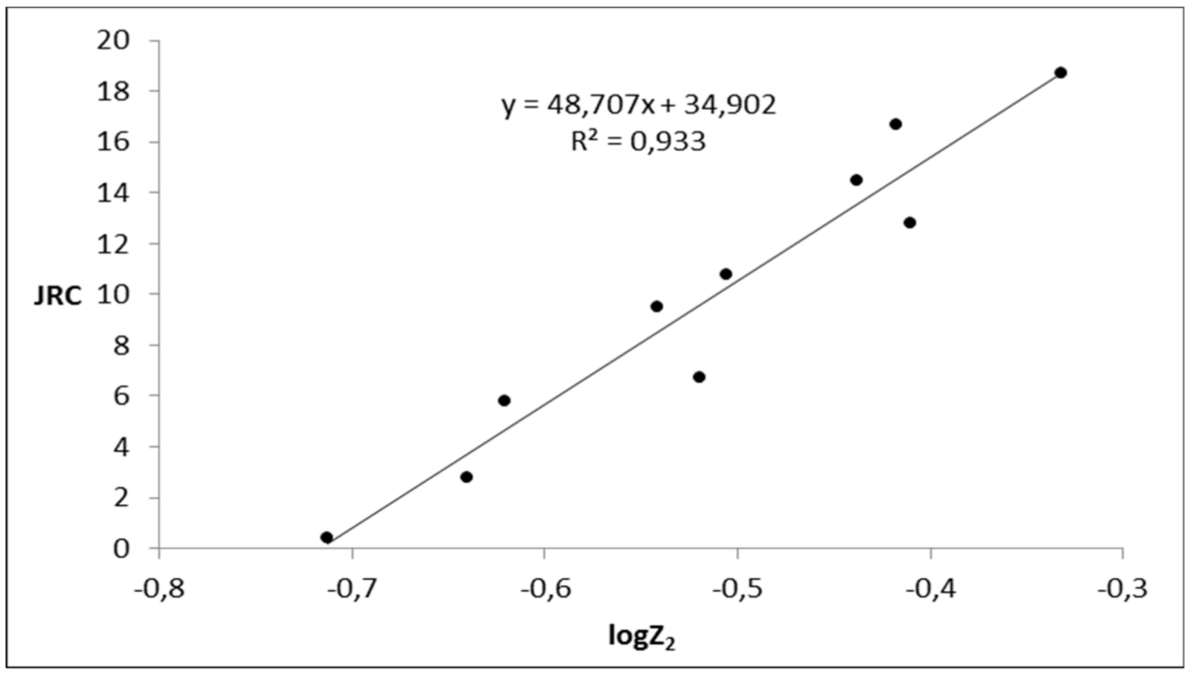
JRC = 48.707 logZ₂ + 37.912,

(10)

with R² = 0.933. The original Barton and Choubey’s [4] image depicting the ten standard JRC profiles was used. The graph of Figure 1 was drawn based on 1024 sampling points for each of these profiles after subtracting the linear trend. The digitalization was done with Wolfram Mathematica. It was only verified that the digitized images coincide visually with Barton and Choubey’s profiles having involved no further fine tuning of the digitization. Apparently, the result depends on both sampling and the quality of image. This is in keeping with the very notion of the standard profiles. Besides, the goal of this paper is not a refined JRC-logZ₂ (or similar) relationship which will just increase R² by a few second decimal units. It is noted that, the various sources of error are discussed in Gao and Wong [8].

Since Tse and Cruden [3], numerous other researchers have either evaluated the existing methods for estimating the JRC coefficient or proposed new ones [7,9,10,11,12,13,14,15,16,17,18,19,20,21,22], e.g., Yang et al. [12] and Yu and Vayssade [7] found R² = 0.986 and 0.910 for the JRC-logZ₂ relationship respectively. However, the Z₂ characteristic remains the most popular one, apparently due to its simplicity and efficiency. A review of these methods is out of scope of the present paper. In this respect, the authors suggest the works done by Li and Zhang [13] and Li and Huang [14]. Instead, the present work intends to embed the estimation of the joint roughness coefficient (JRC) in the framework of the random fields. The random field method is a probabilistic approach to geotechnical problems which involves modeling the spatial variability of the pertinent physical quantities as a fundamental part of the (assumed) underlying probabilistic structure.

2. Methods

The geometric description uses the information contained in the details of the shape of the curve to provide a measure of roughness in a deterministic way. There are many levels of complexity in the geometric description of the profile going all the way to fractal geometry. A recent literature review of empirical equations for estimating JRC by using the fractal dimension D has been offered by Li and Huang [14]. As mentioned above, an elementary and attractive choice is to use the quantity Z₂ defined by Equation (3).

On the other hand, in statistical description, roughness is understood as the estimated value of a certain statistic, treating the profile as a collection of events that obey an underlying probabilistic structure. The autocorrelation function (ACF; Equation (8)) is an example of such a statistic. For example, for zero correlation distance (Δx = 0), the correlation function computes an estimate of the variance σ² of the profile regarding the height y at each point x as a random variable with a fixed variance.

In Tse and Cruden [3], the structure function (SF) defined by Equation (9) has been correlated with the JRC value of the ten standard profiles, which treated Δx as fixed and equal to the length of the interval between two successive sampling points. This showed that it is as good an index as Z₂. This is not surprising because if Δx is the sampling interval, the discrete version of Equations (8) and (9) essentially coincide. Still, the statistical information contained in the ACF as a function over its entire natural range (−L/2, L/2) has neither been exploited nor been put in a statistical framework. This is done herein with the statistical description of roughness based on random fields. In this respect, a profile as a whole is regarded as a single realization of an underlying probabilistic structure where the function ACF(Δx) over the whole of its natural range (−L/2, L/2) is assumed to have a fixed and pre-defined form. This form is denoted by C(Δx) and called the variance function of the random field [23]. The exact definitions are given below.

A function y over −∞ ≤ x ≤ ∞ is a (stationary Gaussian) random field if every number y(x) is a Gaussian random variable with (constant) mean value μ and point-variance σ², i.e.,

E[y(x)] = μ, E[y(x)²] = μ² + σ²,

(11)

where, E[…] denotes the expectation value of the quantity inside the brackets over a large number of realizations of the random field, and every two random variables y(x), y(x + Δx) (associated with two different positions x, x + Δx along the interval) are correlated in a given manner, i.e.,

E[y(x) y(x + Δx)] = μ² + C(Δx),

(12)

These define completely the Gaussian random field. The variance function C(Δx) can be chosen in a variety of ways depending on the nature of the quantity being attempted to model. Clearly, C(0) = σ² by Equations (11) and (12). Therefore, defining the normalized variance function:

ρ(Δx) = C(Δx)/C(0),

(13)

which satisfies ρ(0) = 1. The coordinates in the description of the profiles are chosen so that the mean value μ is zero, so there is no difference between the autocorrelation and variance function of the profile.

A very convenient choice is the Gaussian variance function:

ρ(Δx) = exp[−π(Δx)²/θ²]

(14)

The spatial correlation length θ is defined by

$$\theta ={\displaystyle {\int }_{-\infty }^{\infty }\rho (\Delta x)d(\Delta x)}=2{\displaystyle {\int }_0^{\infty }\rho (\Delta x)d(\Delta x)}$$

(15)

(e.g., see [23,24]) noting that the variance function is even.

It is also noted, that the correlation length is related to the value of the derivatives of the variance function at zero. In particular the value of the second derivative reads:

−ρ”(0) = 2π/θ²

(16)

The integral definition above defines, for any variance function, a macro-scale, while the derivative definition defines a micro-scale. These definitions are usual in other areas where correlation functions are used, e.g., in the theory of turbulence [25]. In general, if the micro-scale can be defined at all, they could be entirely different. The fact that they are both related to the single length θ is of course due to the fact that the model variance function used here involves by definition the single length θ. This feature is realized, in some sense, by the roughness profiles. The argument is as follows.

Consider the Z₂ characteristic defined in Equation (3). If y(x) is a random field, then the index (Z₂)² is a random variable. It can be easily shown that its expectation value is:

E[(Z₂)²] = −σ² ρ”(0) = 2πσ²/θ²,

(17)

The index (Z₂)² can be regarded as a statistic that estimates the value of the (a priori fixed) quantity 2πσ²/θ². In all, in regard of estimates:

Z₂ ∝ σ/θ,

(18)

It is also reminded that Z₂ correlates very well with the roughness coefficient JRC, which must be related to both the macro- and micro-scale of the profile. This recalls the almost perfect correlations found by Tse and Cruden [3], Yang et al. [12] and Yu and Vayssade [7]. However, Z₂ is rather related more to the micro-scales of the profile than to the macro-scales, due to the derivative involved in its definition. Therefore, it is concluded that, first, a single length may be adequate when modelling a roughness profile with a random field and second, that the quantity σ/θ is a good candidate for quantifying the roughness coefficient JRC in the framework of the random fields.

3. Results

3.1. The σ/θ Ratio as an Estimate for JRC Coefficient

Clearly, a direct way to determine σ and θ for a given profile is needed. In this respect, the function ACF(Δx) defined above must first be calculated. This is a priori even function that needs to be determined for Δx in the interval (0, L/2). The point-variance σ² is estimated by ACF(0), whilst θ is extracted from the normalized autocorrelation function ACF(Δx)/ACF(0).

Explicitly, these quantities are constructed from the profile as follows. As mentioned above the sampled profile is a sequence of N = 1024 numbers: y_n for n = 0, 1, …, 1023. The Fourier transform Y_k of the profile y_n is defined by:

$$Y_k={\displaystyle \sum _{n=0}^{N-1}{y}_n\hspace{0.17em}{e}^{-i2\pi \frac{n k}{N}}},$$

(19)

where, k = 0, 1, …, N − 1 are the wave-numbers. Then, ACF(Δx) is the Fourier transform of the magnitude-square of Y_k:

$$ACF(\Delta x)={\displaystyle \sum _{k=0}^{N-1}\frac{|Y_k{|}^2}{N^2}\hspace{0.17em}{e}^{-i2\pi \frac{mk}{N}}},$$

(20)

The correlation distance Δx is of course discrete and is evaluated at the points m·10/N cm, where m is an integer, having divided the 10 cm length of the profile into N = 1023 equally spaced intervals. The ACF(Δx) so defined is a periodic function of period 10 cm. As mentioned above, ACF(Δx) is an even function thus essentially exists in the interval (0, 5 cm) of correlation distances.

The point-variance σ² of the ten standard profiles along with their actual JRC coefficients is given in

Table 1. The point-variance of the ten standard profiles along with their actual joint roughness coefficient (JRC) coefficients.

Profile No.	Real JRC	σ2 (cm2)
1	0.4	0.0002092
2	2.8	0.000372183
3	5.8	0.000969378
4	6.7	0.001708827
5	9.5	0.006983672
6	10.8	0.037012614
7	12.8	0.016019078
8	14.5	0.032283009
9	16.7	0.013746304
10	18.7	0.008309631

.

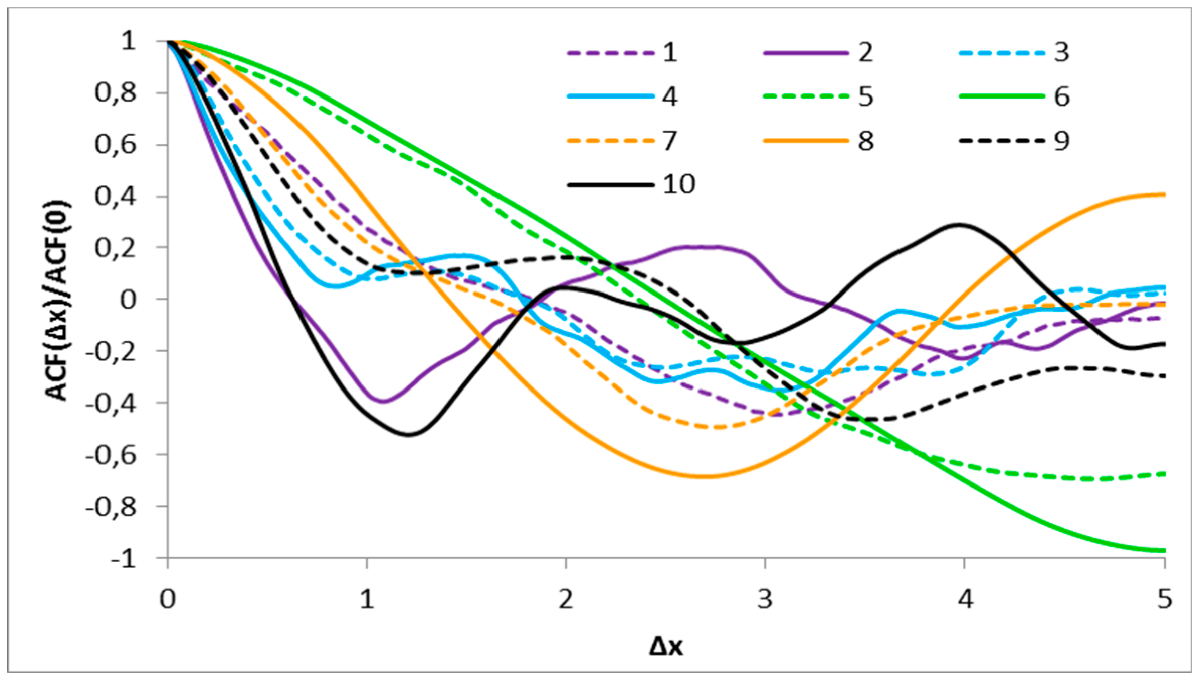
The normalized autocorrelation functions ACF(Δx)/ACF(0) as function of the distance Δx from 0 cm to 5 cm are shown in Figure 2 (labelled by the number of the profile).

The very form of these functions is quite telling. It is observed, for example, that the profiles Nο. 5 and 6 i.e., corresponding to JRC in the range 8–10 and 10–12 respectively, hardly differ in terms of spatial variability, which is also a large scale one. Their essential difference was the magnitude of waviness, measured by the point-variance σ². This is essentially visible in the profiles. Less obvious is the fact that the JRC ranges 2–4 and 18–20 (profile Nο. 2 and 10 respectively) appear to correspond to similar spatial variability, the difference again lying in the point-variance. The value of the length θ for each profile was extracted by fitting the model (Gaussian) normalized variance function ρ(Δx) given above to the normalized autocorrelation function ACF(Δx)/ACF(0).

The values of the spatial correlation length θ associated with each model function ρ(Δx) are given in

Table 2. The values of the spatial correlation length θ associated with each model function ρ(Δx).

Real JRC	θ (cm)	σ/θ
0.4	1.497	0.0097
2.8	0.599	0.0322
5.8	0.952	0.0327
6.7	0.763	0.0542
9.5	2.540	0.0329
10.8	2.731	0.0704
12.8	1.383	0.0915
14.5	1.596	0.1126
16.7	1.216	0.0964
18.7	0.684	0.1332

. These values result from the best fit of each ACF(Δx)/ACF(0) by the respective model function ρ(Δx). Along with them is given the ratio σ/θ, which is our proposal for the JRC coefficient in the random field theory.

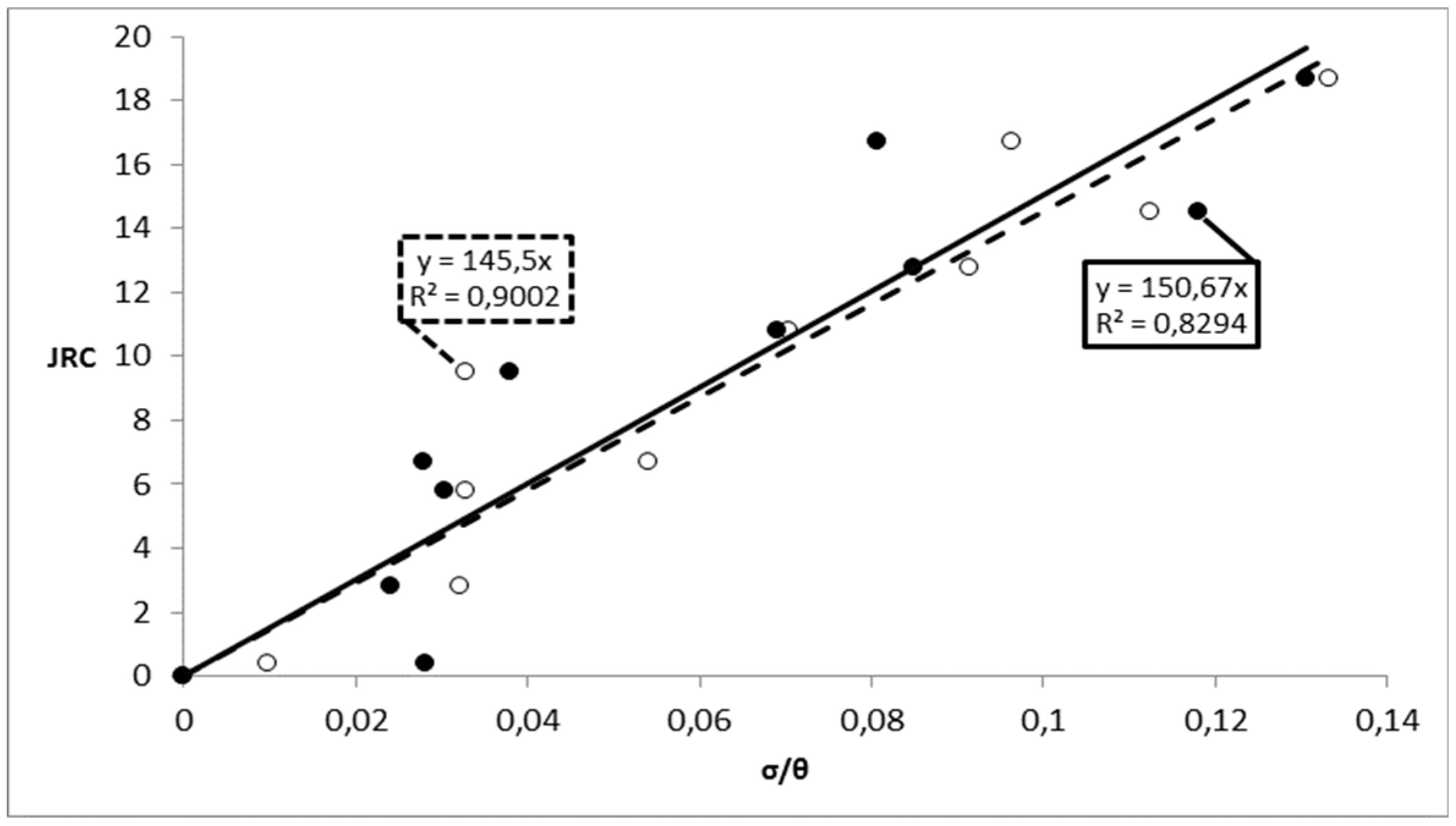
Characteristic of the autocorrelation functions of the profiles is the negative part. Negative parts always occur in the autocorrelation function of a single realization, even if the random field belongs by construction to a specific type, e.g., Gaussian with Gaussian correlations. Therefore, if one is given a single realization of the field, the best way to proceed is by best fitting the obtained correlation/variance function to suitable model function. The Gaussian model correlation used here was chosen among various simple models (e.g., Markovian, white noise, triangular and cubic correlations; see [23]) as the one which performed the best. The quantity σ/θ is given in Table 2 for each roughness coefficient JRC. Moreover, the JRC-σ/θ relationship has been drawn in Figure 3. The R-squared of this relationship was only 3% smaller than the respective one given in Figure 1, also by the authors, for the respective JRC-logZ₂ relationship. Both relationships have been extracted from the same figure (Barton and Choubey’s [4]) without involving fine tuning of the digitization.

It should be noted that, not all of the waviness of the correlation functions, and their negative parts shown in Figure 2, need to be an artifact of the single realization. The cases of JRC 8-10, 10-12 and 14-16 exhibited a more deterministic tendency for negative values and a different pattern than most of the other cases. Clearly, the single-parameter model variance function in Equation (14) is too simple to cover all forms of behavior exhibited by the profiles. A two- or three-parameter model function is required. This shall be the subject of future work.

3.2. Stability of σ/θ as a Roughness Measure

Estimating roughness from the image of a rock surface entails errors due to the quality of the image and its digitation. A simple test as to the behavior of the roughness measures is to calculate the index Z₂ and our index σ/θ and compare the results for the two cases of images. In this respect, the original JRC profiles given in Barton and Choubey [4] and the respective ones reproduced by Tse and Cruden [3] have been used. It is noted that, when the pages containing the standard JRC profiles are printed in A4 paper using the “actual size” option of printer, the linear scale (accompanying the profiles) of 10 cm in Barton and Choubey [4] measured (approximately) 6 cm, whilst the same scale of 10 cm in Tse and Cruden [3] measured just 3 cm. It is also reminded that, none of these raster images of the late 1970s meet the quality standards of today (e.g., the quality of vector images). The profiles of both images were analyzed in the exact same way. The results have been presented below.

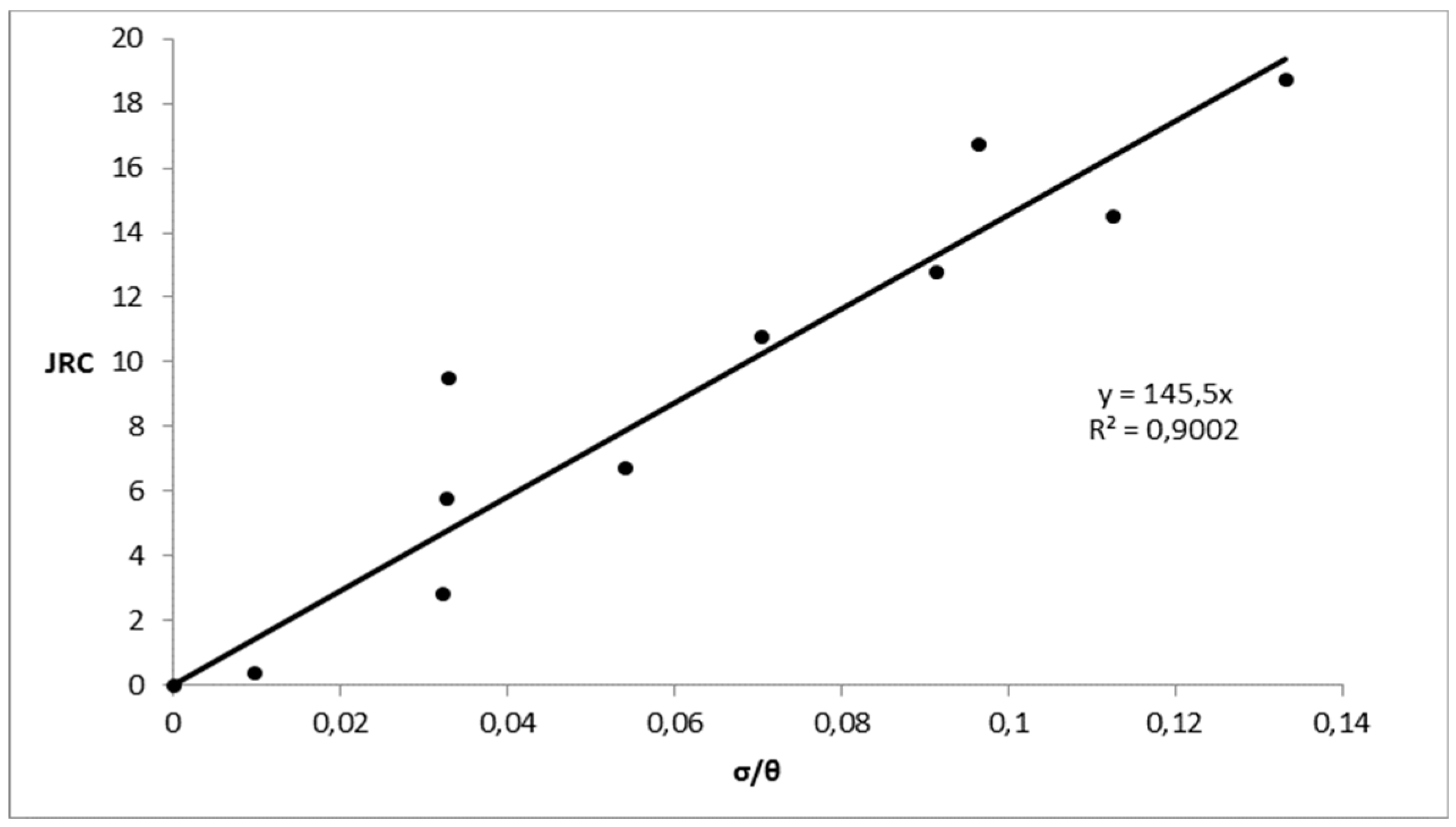
The JRC-logZ₂ relationships extracted by Tse and Cruden’s [3] and Barton and Choubey’s [4] image are shown together in Figure 4, the latter has also be drawn in Figure 1. From Figure 4, it is clear that, the different images have given incomparable estimates for the roughness. This is of particular importance because the same Z₂ value led to complete JRC values.

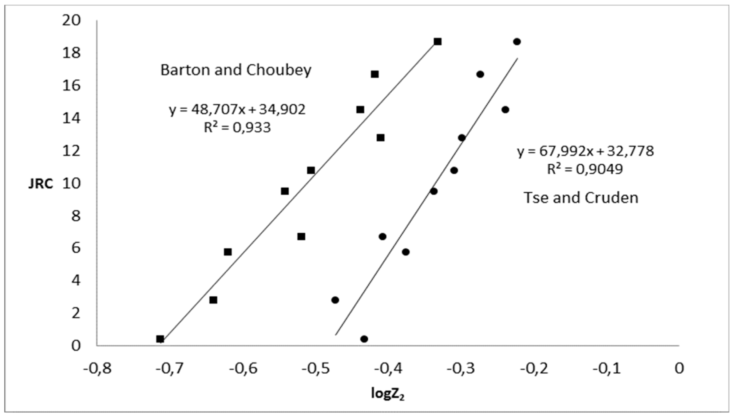
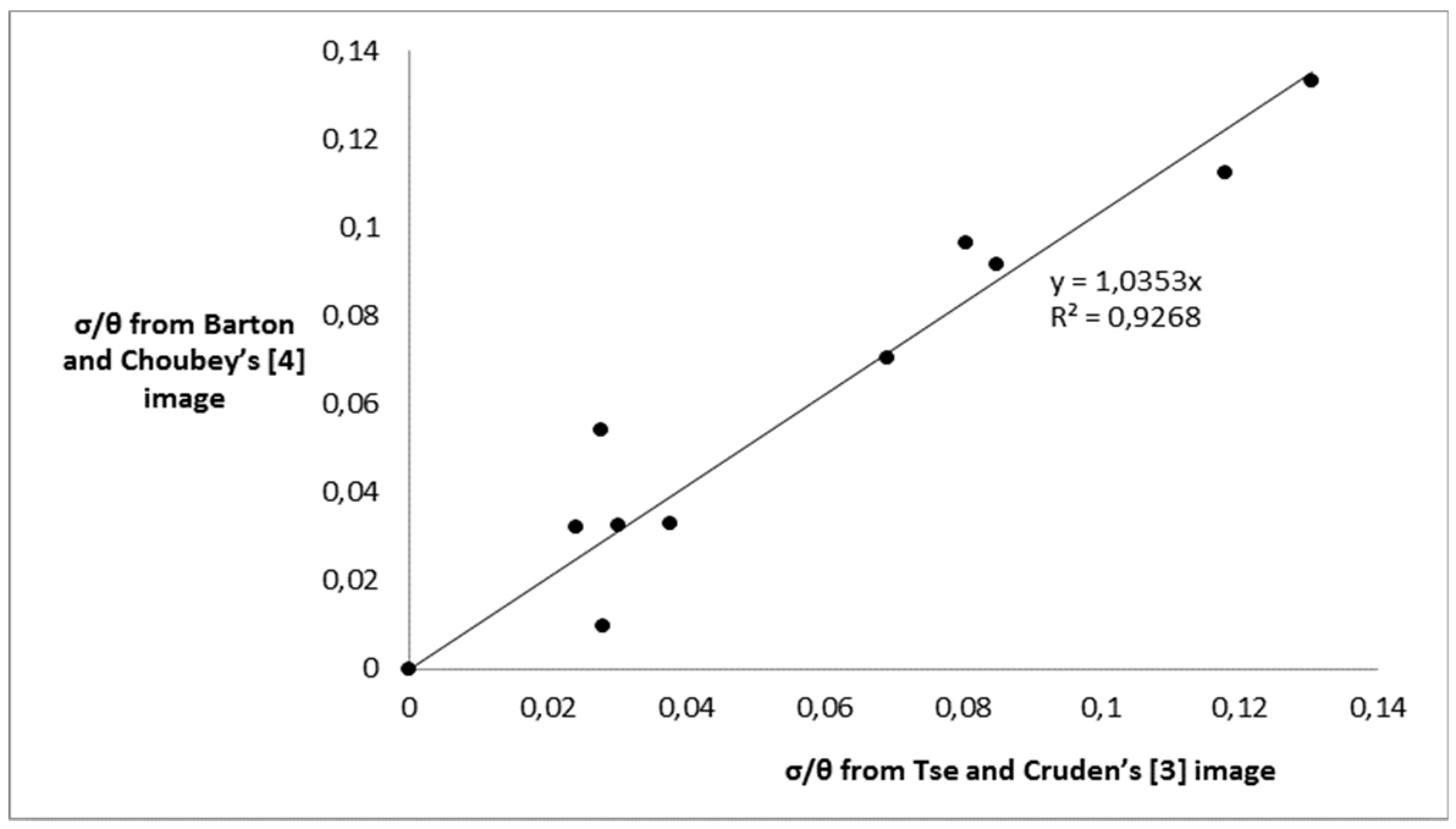
The same has been done but for the JRC-σ/θ relationship. As shown in Figure 5, there is a much greater consistency between the estimates. The level of consistency is additionally shown by plotting the two sets of results against each other. Figure 6 shows the results for logZ₂, whilst Figure 7 shows the results for the σ/θ index introduced in present work. For the case of σ/θ, the higher R² value has been noticed, and also the proximity of the slope of the best fit to the value of 1. The reason why the σ/θ index appears to be more stable than the index Z₂ might be described as follows. Z₂ contains the information contained in ACF(Δx) for equal Δx to the length of the interval between sampling points, i.e., the infinitesimal interval of the given digitation. On the other hand, θ is estimated employing the information contained in ACF(Δx) over all meaningful correlation distances. Apparently, the latter feature operates as a regularizing factor smoothing those errors present in the Z₂ estimate.

3.3. Obtaining θ through JRC

As mentioned earlier, this work intends to embed the estimation of the joint roughness coefficient in the framework of random fields. In this respect, JRC is estimated through σ and θ, or better through the σ/θ ratio. However, the present work could also be useful in an advanced probabilistic rock slope stability analysis [26] based on random fields, considering that the Barton-Bandis criterion [27] has been adopted. In order for a random field analysis to be performed, the spatial correlation length θ of joint roughness must be known. If now the JRC coefficient and the variance σ of the profile are known, the spatial correlation length θ can be obtained from the best fit relation of Figure 3, as follows:

Θ = 145.5 σ/JRC,

(21)

The JRC coefficient can be obtained directly through tilt tests, push or pull tests, or matching roughness profiles [4], whilst the variance σ can be obtained from inspection of the digitized profile.

4. Discussion

The authors revisited the problem of determining the joint roughness coefficient (JRC) included in the Barton-Bandis failure criterion from the point of view of digitalized profiles of discontinuities. However, numerous indices have been correlated with JRC, with the geometric characteristic Z₂ being, probably, the most popular one. Based on the international literature, the statistical measure SF (Structure Function), has been a good alternative giving also very strong correlations with JRC.

As the random fluctuation of discontinuities can be considered as being random fields, the present paper targeted on embedding the estimation of the joint roughness coefficient (JRC) in the framework of the theory of random fields. The analysis showed that the fluctuation of discontinuities in both micro- and macro scale was related to a single length and more specifically to the spatial correlation length, θ (essential parameter in the theory of random fields). Indeed, it was found that the quantity σ/θ was a good candidate for quantifying the roughness coefficient JRC. Usually, the determination of θ relies on the best fit of a suitably chosen model variance function to the normalized autocorrelation function. The stability of the proposed σ/θ index as a roughness measure was compared against the characteristic Z₂. In this respect, the two indices were applied to images of the same discontinuity profiles and more specifically, the ten standard JRC profiles given by Barton and Choubey [4], but of different quality. From the results, it is clear that the estimates for JRC by the proposed method appear to be much more stable, in contrast to Z₂ or, as explained earlier, SF (structure function).

The fact that the R-squared value for the JRC-σ/θ relationship of Figure 3 (R² = 0.9002), although very strong, was not perfectly strong can be attributed to three main reasons. First, no fine tuning of the digitization of Barton and Choubey’s [4] figure was involved. Second, the ten JRC profiles were representative of the two-dimensional cross-sections, whilst their JRC values were average values referring to the respective three-dimensional fluctuating surface of the rock blocks. Third, despite the versatility of the random field method, the derived θ values depended on the extend of the sampling domain [28,29]. An extensive parallel research conducted by the authors (paper under preparation) indicated that, for eliminating this kind of error in the proposed JRC-σ/θ relationship, a domain at least 35θ in length was required to be considered. Indeed, as the domain length increases (in this respect, the length of discontinuity) the θ value reaches asymptotically its maximum value for the specific random field. This is in agreement with the empirical scale correction relationship suggested by Barton and Bandis [30]:

$${\mathrm{JRC}}_{\mathrm{n}}\approx {\mathrm{JRC}}_{\mathrm{o}}{\left(\frac{{\mathrm{L}}_{\mathrm{n}}}{{\mathrm{L}}_{\mathrm{o}}}\right)}^{-0.02\cdot {\mathrm{JRC}}_{\mathrm{o}}}$$

(22)

where, JRC_n and JRC_o are the joint roughness coefficients corresponding to samples of length L_n and L_o = 10 cm respectively. More specifically, Equation (22) shows that, the JRC_n value decreases as the L_n/L_o ratio increases towards a minimum asymptotic value. On the other hand, as L_n/L_o increases, the σ/θ ratio and thus, the JRC value decreases (recall the JRC-σ/θ relationship in Figure 3) towards a minimum asymptotic value. Based on the θ values given in Table 2, the rock joint profiles should be at least 2 to 9 times longer than the 10 cm of the original Barton and Choubey’s [4] profiles (value depending on the fluctuation pattern of each profile) for effectively determining the JRC.

The above has been supported by the experimental findings of Barton and Choubey [4]. In this respect, Barton and Choubey performed three tilt tests on a 40 × 45 cm joint area (sliding along the long dimension) and they found an (average) joint roughness coefficient value equal to 5.5. The same sample was sawn by Barton and Choubey into 18 samples 4.9 × 9.8 cm in size (samples by 45/9.8 = 4.6 times shorter in the shear direction than the original joint area). The shear direction was marked so that each of the small specimens could be tilt-tested, push-tested and shear box tested in the same direction as the original tilt test of the 45 cm long joint. The results of this investigation are summarized in

Table 3. JRC values obtained by different test methods (see Barton and Choubey [4]) and correction for scale.

Statistical Description of Test Data and JRCn Values	Shear Box 1	Tilt 1	Push 1	Overall
Number of samples tested	18	6	12	36
Mean JRC value, μ	8.69	6.18	10.17	8.76
Standard deviation, σ	1.18	0.66	0.55	1.63
JRCn 2 (Equation (22))	6.67	5.12	7.46	6.71

¹ Not the same samples used in the tilt test were used in the push test, but all samples were tested in the shear box. ² Reduction of the above JRC values to samples 45 cm in length based on Barton and Bandis’s [30] scale correction.

. From the table in question it is inferred that: (i) The (mean) JRC value depends greatly on the type of test; (ii) the standard deviation alone is not a good index for indicating the proper type of test; and (iii) the best estimate was obtained from the tilt test (please compare the JRC_n = 5.12 value with the JRC_n = 5.5 for the 40 × 45 cm joint area). The latter could be attributed to test compatibility, as the 40 × 45 cm joint area was also tested on a tilt test configuration.

For considering the extent of the pattern of fluctuations on the JRC value, the authors suggest that the JRC be determined based on joint profiles of adequate length. This suggestion is independent of the method adopted (i.e., determination of JRC in the field, in the laboratory or based on correlations e.g., with Z₂ or SF). For discontinuities with large scale waviness, apparently, this length should be even greater. A test joint surface length is adequate when considering greater length, as the JRC value remains practically the same.

It is noted that, if the present method is adopted, no correction for the influence of scale on JRC (such as the one proposed by Barton and Bandis [30]; see Equation (22)), is required. However, because of the greater possibility of weaknesses in a large surface, it is likely that the average joint wall compressive strength (JCS) decreases with increasing scale. In this respect, Barton and Bandis’ [30] scale correction for JCS (recall Equation (6)) is suggested. It is additionally mentioned that, Barton and Bandis’s [30] scale correction was derived from shear tests over a ten-fold range of block sizes, involving linear extrapolation outside the block size range 0.1 m to 1 m. On the contrary, the proposed method is straightforward, not involving such procedures.

Finally, as the problem is clearly one dimensional, and since sliding will take place along a specific direction, the final JRC value should be an average value derived from a number of profiles parallel to the direction of sliding. In this respect, the JRC = 145.5 σ/θ relationship is a convenient and reliable tool for such an analysis. Refinement of this relationship based on longer sampling domain lengths is subject matter of future research by the authors, although it is believed that this best fit equation will not dramatically change.

References

1. American Society of Mechanical Engineers. Surface Roughness, Waviness and Lay; ASA B46.1; American Society of Mechanical Engineers: New York, NY, USA, 1955. [Google Scholar]
2. Myers, N.O. Characterization of surface roughness. Wear 1962, 5, 182–189. [Google Scholar] [CrossRef]
3. Tse, R.; Cruden, D.M. Estimating Joint Roughness Coefficients. In Proceedings of the International Journal of Rock Mechanics and Mining Sciences Geomechanics Abstracts; Elsevier: Amsterdam, The Nederland, 1979; Volume 16, pp. 303–307. [Google Scholar]
4. Barton, N.; Choubey, V. The shear strength of rock joints in theory and practice. Rock Mech. 1977, 10, 1–54. [Google Scholar] [CrossRef]
5. Ulusay, R. (Ed.) The ISRM Suggested Methods for Rock Characterization, Testing and Monitoring: 2007–2014; Springer International Publishing: Cham, Switzerland, 2015; ISBN 978-3-319-07712-3. [Google Scholar]
6. Sayles, R.S.; Thomas, T.R. The spatial representation of surface roughness by means of the structure function: A practical alternative to correlation. Wear 1977, 42, 263–276. [Google Scholar] [CrossRef]
7. Yu, X.; Vayssade, B. Joint profiles and their roughness parameters. Int. J. Rock Mech. Min. Sci. Geomech. Abstr. 1991, 28, 333–336. [Google Scholar] [CrossRef]
8. Gao, Y.; Wong, L.N.Y. A Modified Correlation Between Roughness Parameter Z 2 and the JRC. Rock Mech. Rock Eng. 2015, 48, 387–396. [Google Scholar] [CrossRef]
9. Turk, N.; Greig, M.; Dearman, W.; Amin, F.F. Characterization of Rock Joint Surfaces by Fractal Dimension. In Proceedings of the 28th U.S. Symposium on Rock Mechanics (USRMS), Tucson, AZ, USA, 29 June–1 July 1987; Association, A.R.M., Ed.; A. A. Balkema: Rotterdam, The Netherlands, 1987; p. ARMA-87-1223. [Google Scholar]
10. Lamas, L.N. An experimental and analytical study of the roughness of granite joints. In Proceedings of the ISRM International Symposium-EUROCK 96, Turin, Italy, 2–5 September 1996; International Society for Rock Mechanics and Rock Engineering; A. A. Balkema: Rotterdam, The Netherlands, 1996. [Google Scholar]
11. Chen, S.J.; Zhu, W.C.; Zhang, M.S.; Yu, Q.L. Fractal description of rock joints based on digital image processing technique. Chin. J. Geotech. Eng. 2012, 34, 2087–2092. [Google Scholar]
12. Yang, Z.Y.; Lo, S.C.; Di, C.C. Reassessing the Joint Roughness Coefficient (JRC) Estimation Using Z2. Rock Mech. Rock Eng. 2001, 34, 243–251. [Google Scholar] [CrossRef]
13. Li, Y.; Zhang, Y. Quantitative estimation of joint roughness coefficient using statistical parameters. Int. J. Rock Mech. Min. Sci. 2015, 77, 27–35. [Google Scholar] [CrossRef] [Green Version]
14. Li, Y.; Huang, R. Relationship between joint roughness coefficient and fractal dimension of rock fracture surfaces. Int. J. Rock Mech. Min. Sci. 2015, 75, 15–22. [Google Scholar] [CrossRef] [Green Version]
15. Carr, J.R.; Warriner, J.B. Rock mass classification of joint roughness coefficient. In Proceedings of the 28th US Rock Mechanics Symposium, Tucson, AZ, USA, 29 June–1 July 1987; pp. 72–86. [Google Scholar]
16. Bae, D.; Kim, K.; Koh, Y.; Kim, J. Characterization of Joint Roughness in Granite by Applying the Scan Circle Technique to Images from a Borehole Televiewer. Rock Mech. Rock Eng. 2011, 44, 497–504. [Google Scholar] [CrossRef]
17. Askari, M.; Ahmadi, M. Failure Process after Peak Strength of Artificial Joints by Fractal Dimension. Geotech. Geol. Eng. 2007, 25, 631–637. [Google Scholar] [CrossRef]
18. Shitian, Q.S.Z.Z.W.; Runqiu, H. Fractal characteristics of jointed rock mass and its engineering geology significance. J. Eng. Geol. 1993, 2, 14–23. [Google Scholar]
19. Jia, H.Q. Experimental Research on Joint Surface State and the Characteristics of Shear Failure. Ph.D. Thesis, Central South University, Changsha, China, 2011. [Google Scholar]
20. Zhou, C.B.; Xiong, W.L. Relation between joint roughness coefficient and fractal dimension. J. Wuhan Univ. Hydraul. Electr. Eng. 1996, 29, 1195–1197. [Google Scholar]
21. Maerz, N.H.; Franklin, J.A. Roughness scale effect and fractal dimension. In Proceedings of the 1st International Workshop on Scale Effects in Rock Masses, Loen, Norway, 7–8 June 1990; A. A. Balkema: Rotterdam, The Netherlands, 1990; pp. 121–126. [Google Scholar]
22. Liu, S.Y. Fractional dimension method of JRC measurement. Investig. Sci. Technol. 1993, 6, 26–29. [Google Scholar]
23. Fenton, G.; Griffiths, D.V. Risk Assessment in Geotechnical Engineering; Wiley: New York, NY, USA, 2008; ISBN 9780470178201. [Google Scholar]
24. Vanmarcke, E.H. Random Fields: Analysis and Synthesis; MIT Press: Cambridge, MA, USA, 1983. [Google Scholar]
25. Batchelor, G.K. (Ed.) The Theory of Homogeneous Turbulence; Cambridge Monographs on Mechanics and Applied Mathematics; Cambridge University Press: Cambridge, UK, 1953. [Google Scholar]
26. Gravanis, E.; Pantelidis, L.; Griffiths, D.V. An analytical solution in probabilistic rock slope stability assessment based on random fields. Int. J. Rock Mech. Min. Sci. 2014, 71, 19–24. [Google Scholar] [CrossRef]
27. Barton, N.; Bandis, S. Review of predictive capabilities of JRC-JCS model in engineering practice. In Proceedings of the International Symposium on Rock Joints, Loen, Norway, 4–6 June 1990; Barton, N., Stephenson, O., Eds.; CRC Press Book; A. A. Balkema: Rotterdam, The Netherlands, 1990; pp. 603–610. [Google Scholar]
28. Nie, X.; Zhang, T.; Huang, H.; Liu, Z.; Lacasse, S. Scale of Fluctuation for Geotechnical Probabilistic Analysis; IOS Press: Rotterdam, The Netherlands, 2015; pp. 816–821. [Google Scholar]
29. Fenton, G.A. Random field modeling of CPT data. J. Geotech. Geoenviron. Eng. 1999, 125, 486–498. [Google Scholar] [CrossRef]
30. Barton, N.; Bandis, S. Effects of block size on the shear behavior of jointed rock. In Proceedings of the 23rd US Symposium on Rock Mechanics (USRMS), Berkeley, CA, USA, 25–27 August 1982; American Rock Mechanics Association: Richardson, TX, USA, 1982; pp. 739–760. [Google Scholar]
Figure 1. JRC-logZ2 relationship for the ten standard JRC profiles of Barton and Choubey [4].
Geosciences 09 00295 g001
Figure 2. The normalized autocorrelation functions ACFx)/ACF (0) as function of the distance Δx (labelled by the No. of Barton and Choubey’s [4] profile; see also Appendix A).
Geosciences 09 00295 g002
Figure 3. The JRC-σ/θ relationship.
Geosciences 09 00295 g003
Figure 4. Graph comparing the JRC-logZ2 relationship extracted from Tse and Cruden’s [3] and Barton and Choubey’s [4] image.
Geosciences 09 00295 g004
Figure 5. Graph comparing the JRC-σ/θ relationship extracted from Barton and Choubey’s [4] and Tse and Cruden’s [3] image (white and black dots respecrively).
Geosciences 09 00295 g005
Figure 6. Graph comparing the logZ2 values obtained from Tse and Cruden’s [3] and Barton and Choubey’s [4] image.
Geosciences 09 00295 g006
Figure 7. Graph comparing the σ/θ values obtained from Tse and Cruden’s [3] and Barton and Choubey’s [4] image.
Geosciences 09 00295 g007