Comparison of Hydraulic and Tracer Tomography for Discrete Fracture Network Inversion


Abstract
:1. Introduction
2. Methodology
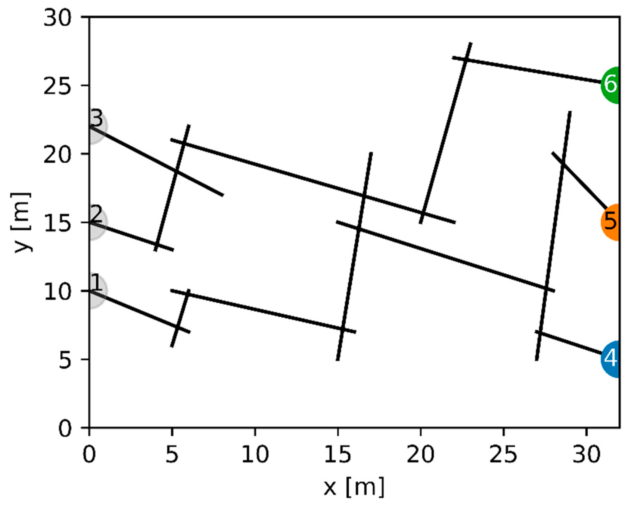
2.1. DFN Case Study
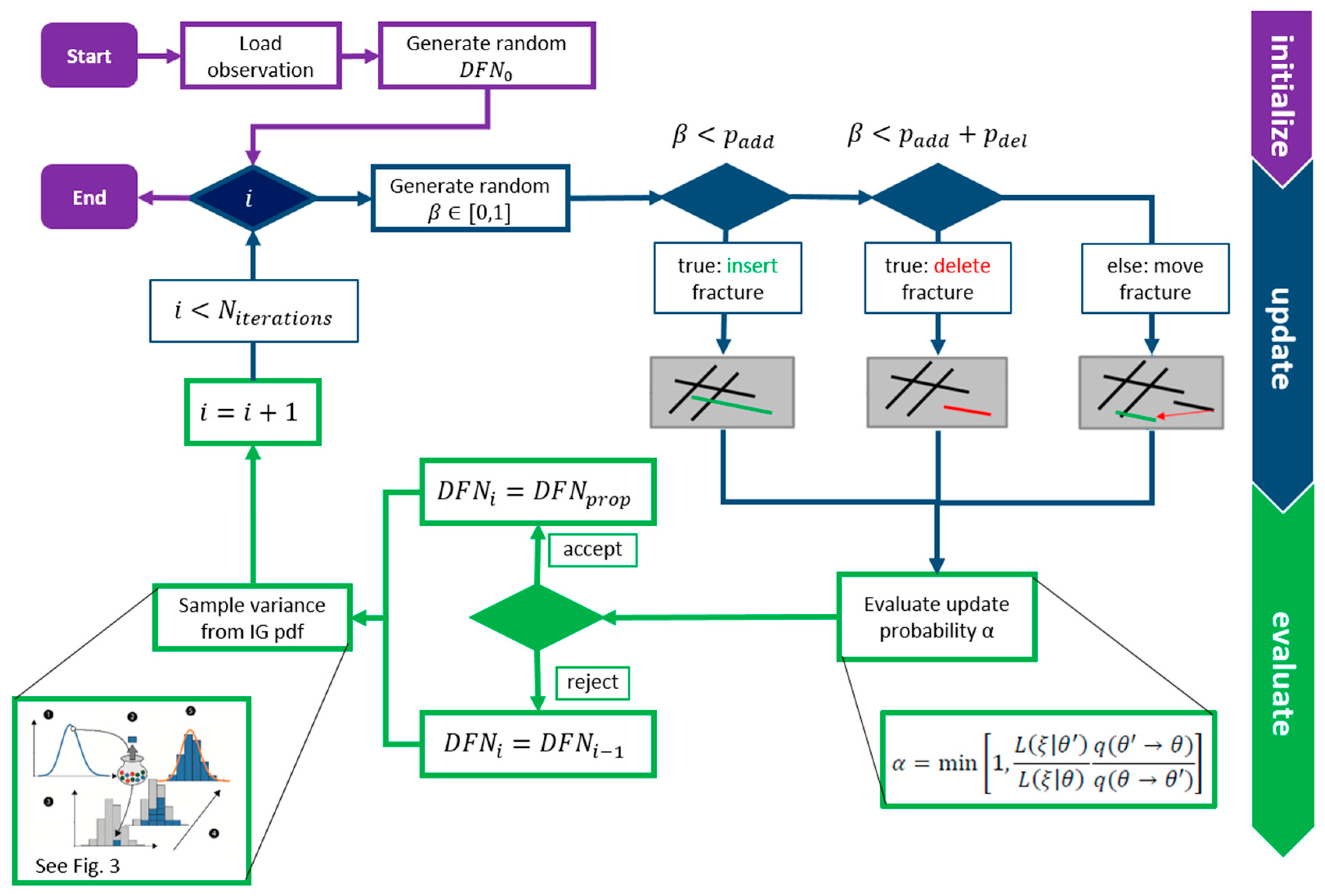
2.2. Transdimensional Inversion
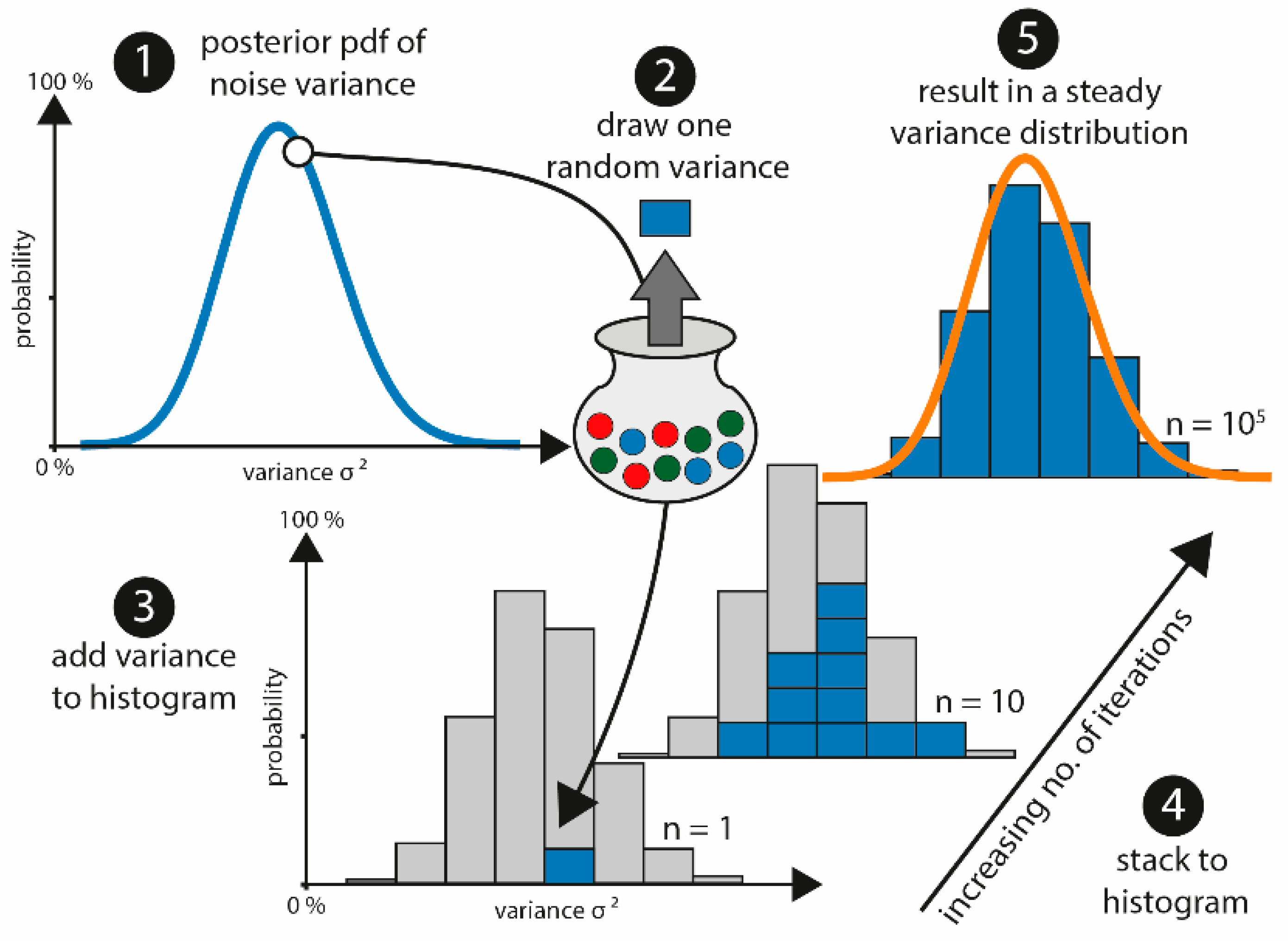
2.3. Estimation of the Noise Variance
3. Results
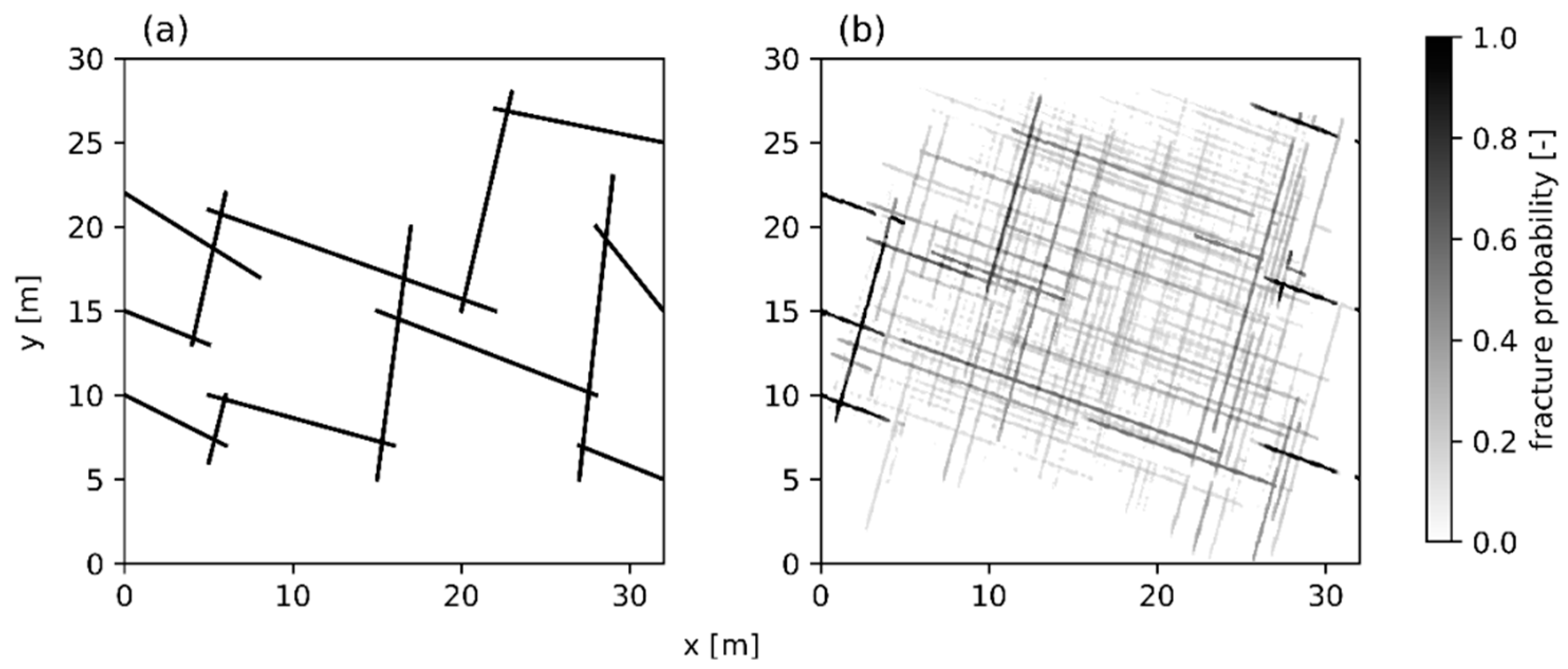
3.1. Results of the DFN Inversion
3.2. Results Estimating the Noise Variance
4. Discussion and Conclusions
Author Contributions
Funding
Acknowledgments
Conflicts of Interest
References
- Berg, S.J.; Illman, W.A. Three-dimensional transient hydraulic tomography in a highly heterogeneous glaciofluvial aquifer-aquitard system. Water Resour. Res. 2011, 47. [Google Scholar] [CrossRef]
- Brauchler, R.; Hu, R.; Hu, L.; Jiménez, S.; Bayer, P.; Dietrich, P.; Ptak, T. Rapid field application of hydraulic tomography for resolving aquifer heterogeneity in unconsolidated sediments. Water Resour. Res. 2013, 49. [Google Scholar] [CrossRef]
- Cardiff, M.; Barrash, W.; Kitanidis, P.K. A field proof-of-concept of aquifer imaging using 3-D transient hydraulic tomography with modular, temporarily-emplaced equipment. Water Resour. Res. 2012, 48. [Google Scholar] [CrossRef] [Green Version]
- Jiménez, S.; Brauchler, R.; Bayer, P. A new sequential procedure for hydraulic tomographic inversion. Adv. Water Resour. 2013, 62, 59–70. [Google Scholar] [CrossRef]
- Illman, W.A. Hydraulic tomography offers improved imaging of heterogeneity in fractured rocks. Groundwater 2014, 52, 659–684. [Google Scholar] [CrossRef]
- Zha, Y.; Yeh, T.C.J.; Illman, W.A.; Zeng, W.; Zhang, Y.; Sun, F.; Shi, L. A Reduced-Order Successive Linear Estimator for Geostatistical Inversion and its Application in Hydraulic Tomography. Water Resour. Res. 2018, 54, 1616–1632. [Google Scholar] [CrossRef]
- Hu, L.; Bayer, P.; Alt-Epping, P.; Tatomir, A.; Sauter, M.; Brauchler, R. Time-lapse pressure tomography for characterizing CO2 plume evolution in a deep saline aquifer. Int. J. Greenh. Gas Control 2015, 39, 91–106. [Google Scholar] [CrossRef]
- Hu, L.; Bayer, P.; Brauchler, R. Detection of carbon dioxide leakage during injection in deep saline formations by pressure tomography. Water Resour. Res. 2016, 52, 5676–5686. [Google Scholar] [CrossRef]
- Vesselinov, V.V.; Neuman, S.P.; Illman, W.A. Three-dimensional numerical inversion of pneumatic cross-hole tests in unsaturated fractured tuff: 1. Methodology and borehole effects. Water Resour. Res. 2001, 37, 3001–3017. [Google Scholar] [CrossRef]
- Ni, C.-F.; Yeh, T.-C.J. Stochastic inversion of pneumatic cross-hole tests and barometric pressure fluctuations in heterogeneous unsaturated formations. Adv. Water Resour. 2008, 31, 1708–1718. [Google Scholar] [CrossRef]
- Datta-Gupta, A.; Yoon, S.; Vasco, D.W.; Pope, G.A. Inverse modeling of partitioning interwell tracer tests: A streamline approach. Water Resour. Res. 2002, 38. [Google Scholar] [CrossRef]
- Jiménez, S.; Mariethoz, G.; Brauchler, R.; Bayer, P. Smart pilot points using reversible-jump Markov-chain Monte Carlo. Water Resour. Res. 2016, 52, 3966–3983. [Google Scholar] [CrossRef] [Green Version]
- Ma, R.; Zheng, C.; Zachara, J.M.; Tonkin, M. Utility of bromide and heat tracers for aquifer characterization affected by highly transient flow conditions. Water Resour. Res. 2012, 48. [Google Scholar] [CrossRef]
- Doetsch, J.; Linde, N.; Vogt, T.; Binley, A.; Green, A.G. Imaging and quantifying salt-tracer transport in a riparian groundwater system by means of 3D ERT monitoring. Geophysics 2012, 77, B207–B218. [Google Scholar] [CrossRef] [Green Version]
- Jardani, A.; Revil, A.; Dupont, J. Stochastic joint inversion of hydrogeophysical data for salt tracer test monitoring and hydraulic conductivity imaging. Adv. Water Resour. 2013, 52, 62–77. [Google Scholar] [CrossRef]
- Jougnot, D.; Jiménez-Martínez, J.; Legendre, R.; Le Borgne, T.; Méheust, Y.; Linde, N. Impact of small-scale saline tracer heterogeneity on electrical resistivity monitoring in fully and partially saturated porous media: Insights from geoelectrical milli-fluidic experiments. Adv. Water Resour. 2018, 113, 295–309. [Google Scholar] [CrossRef] [Green Version]
- Singha, K.; Gorelick, S.M. Saline tracer visualized with three-dimensional electrical resistivity tomography: Field-scale spatial moment analysis. Water Resour. Res. 2005, 41. [Google Scholar] [CrossRef]
- Hermans, T.; Wildemeersch, S.; Jamin, P.; Orban, P.; Brouyère, S.; Dassargues, A.; Nguyen, F. Quantitative temperature monitoring of a heat tracing experiment using cross-borehole ERT. Geothermics 2015, 53, 14–26. [Google Scholar] [CrossRef] [Green Version]
- Schwede, R.L.; Li, W.; Leven, C.; Cirpka, O.A. Three-dimensional geostatistical inversion of synthetic tomographic pumping and heat-tracer tests in a nested-cell setup. Adv. Water Resour. 2014, 63, 77–90. [Google Scholar] [CrossRef]
- Somogyvári, M.; Bayer, P.; Brauchler, R. Travel-time-based thermal tracer tomography. Hydrol. Earth Syst. Sci. 2016, 20, 1885–1901. [Google Scholar] [CrossRef] [Green Version]
- Klepikova, M.V.; Le Borgne, T.; Bour, O.; Gallagher, K.; Hochreutener, R.; Lavenant, N. Passive temperature tomography experiments to characterize transmissivity and connectivity of preferential flow paths in fractured media. J. Hydrol. 2014, 512, 549–562. [Google Scholar] [CrossRef] [Green Version]
- Cardiff, M.; Barrash, W.; Kitanidis, P.K. Hydraulic conductivity imaging from 3-D transient hydraulic tomography at several pumping/observation densities. Water Resour. Res. 2013, 49, 7311–7326. [Google Scholar] [CrossRef] [Green Version]
- Bohling, G.C.; Butler, J.J.; Zhan, X.; Knoll, M.D. A field assessment of the value of steady shape hydraulic tomography for characterization of aquifer heterogeneities. Water Resour. Res. 2007, 43. [Google Scholar] [CrossRef] [Green Version]
- Paradis, D.; Gloaguen, E.; Lefebvre, R.; Giroux, B. A field proof-of-concept of tomographic slug tests in an anisotropic littoral aquifer. J. Hydrol. 2016, 536, 61–73. [Google Scholar] [CrossRef]
- Somogyvári, M.; Bayer, P. Field validation of thermal tracer tomography for reconstruction of aquifer heterogeneity. Water Resour. Res. 2017, 53, 5070–5084. [Google Scholar] [CrossRef]
- Tso, C.H.M.; Zha, Y.; Yeh, T.C.J.; Wen, J.C. The relative importance of head, flux, and prior information in hydraulic tomography analysis. Water Resour. Res. 2016, 52, 3–20. [Google Scholar]
- Zhao, Z.; Illman, W.A.; Yeh, T.C.J.; Berg, S.J.; Mao, D. Validation of hydraulic tomography in an unconfined aquifer: A controlled sandbox study. Water Resour. Res. 2015, 51, 4137–4155. [Google Scholar] [CrossRef]
- Hu, R.; Brauchler, R.; Herold, M.; Bayer, P. Hydraulic tomography analog outcrop study: Combining travel time and steady shape inversion. J. Hydrol. 2011, 409, 350–362. [Google Scholar] [CrossRef]
- Hao, Y.; Yeh, T.C.J.; Xiang, J.; Illman, W.A.; Ando, K.; Hsu, K.C.; Lee, C.H. Hydraulic tomography for detecting fracture zone connectivity. Groundwater 2008, 46, 183–192. [Google Scholar] [CrossRef]
- Illman, W.A. Lessons learned from hydraulic and pneumatic tomography in fractured rocks. Procedia Environ. Sci. 2015, 25, 127–134. [Google Scholar] [CrossRef]
- Illman, W.A.; Liu, X.; Takeuchi, S.; Yeh, T.C.J.; Ando, K.; Saegusa, H. Hydraulic tomography in fractured granite: Mizunami Underground Research site, Japan. Water Resour. Res. 2009, 45. [Google Scholar] [CrossRef] [Green Version]
- Zha, Y.; Yeh, T.-C.J.; Illman, W.A.; Tanaka, T.; Bruines, P.; Onoe, H.; Saegusa, H. What does hydraulic tomography tell us about fractured geological media? A field study and synthetic experiments. J. Hydrol. 2015, 531, 17–30. [Google Scholar] [CrossRef]
- Dong, Y.; Fu, Y.; Yeh, T.C.J.; Wang, Y.L.; Zha, Y.; Wang, L.; Hao, Y. Equivalence of Discrete Fracture Network and Porous Media Models by Hydraulic Tomography. Water Resour. Res. 2019. [Google Scholar] [CrossRef]
- Wen, J.C.; Chen, J.L.; Yeh, T.C.J.; Wang, Y.L.; Huang, S.Y.; Tian, Z.; Yu, C.Y. Redundant and non-redundant information for Model Calibration or Hydraulic Tomography. Groundwater 2019. [Google Scholar] [CrossRef] [PubMed]
- Wang, X.; Jardani, A.; Jourde, H. A hybrid inverse method for hydraulic tomography in fractured and karstic media. J. Hydrol. 2017, 551, 29–46. [Google Scholar] [CrossRef]
- Brauchler, R.; Böhm, G.; Leven, C.; Dietrich, P.; Sauter, M. A laboratory study of tracer tomography. Hydrogeol. J. 2013, 21, 1265–1274. [Google Scholar] [CrossRef]
- Fischer, P.; Jardani, A.; Wang, X.; Jourde, H.; Lecoq, N. Identifying Flow Networks in a Karstified Aquifer by Application of the Cellular Automata-Based Deterministic Inversion Method (Lez Aquifer, France). Water Resour. Res. 2017, 53, 10508–10522. [Google Scholar] [CrossRef]
- Fischer, P.; Jardani, A.; Jourde, H.; Cardiff, M.; Wang, X.; Chedeville, S.; Lecoq, N. Harmonic pumping tomography applied to image the hydraulic properties and interpret the connectivity of a karstic and fractured aquifer (Lez aquifer, France). Adv. Water Resour. 2018, 119, 227–244. [Google Scholar] [CrossRef]
- Fischer, P.; Jardani, A.; Lecoq, N. Hydraulic tomography of discrete networks of conduits and fractures in a karstic aquifer by using a deterministic inversion algorithm. Adv. Water Resour. 2018, 112, 83–94. [Google Scholar] [CrossRef]
- Somogyvári, M.; Jalali, M.; Jimenez Parras, S.; Bayer, P. Synthetic fracture network characterization with transdimensional inversion. Water Resour. Res. 2017, 53, 5104–5123. [Google Scholar] [CrossRef]
- Dorn, C.; Linde, N.; Le Borgne, T.; Bour, O.; Baron, L. Single-hole GPR reflection imaging of solute transport in a granitic aquifer. Geophys. Res. Lett. 2011, 38. [Google Scholar] [CrossRef] [Green Version]
- Chuang, P.-Y.; Chia, Y.; Chiu, Y.-C.; Teng, M.-H.; Liou, S.Y.H. Mapping fracture flow paths with a nanoscale zero-valent iron tracer test and a flowmeter test. Hydrogeol. J. 2018, 26, 321–331. [Google Scholar] [CrossRef]
- Ziegler, M.; Loew, S.; Moore, J.R. Distribution and inferred age of exfoliation joints in the Aar Granite of the central Swiss Alps and relationship to Quaternary landscape evolution. Geomorphology 2013, 201, 344–362. [Google Scholar] [CrossRef]
- Jalali, M. Thermo-Hydro-Mechanical Behavior of Conductive Fractures Using a Hybrid Finite Difference—Displacement Discontinuity Method; University of Waterloo Library: Waterloo, ON, Canada, 2013. [Google Scholar]
- Afshari Moein, M.J.; Somogyvári, M.; Valley, B.; Jalali, M.; Loew, S.; Bayer, P. Fracture Network Characterization Using Stress-Based Tomography. J. Geophys. Res. Solid Earth 2018, 123, 9324–9340. [Google Scholar] [CrossRef]
- Green, P.J. Reversible jump Markov chain Monte Carlo computation and Bayesian model determination. Biometrika 1995, 82, 711–732. [Google Scholar] [CrossRef]
- Metropolis, N.; Rosenbluth, A.W.; Rosenbluth, M.N.; Teller, A.H.; Teller, E. Equation of state calculations by fast computing machines. J. Chem. Phys. 1953, 21, 1087–1092. [Google Scholar] [CrossRef]
- Denison, D.G.; Holmes, C.C.; Mallick, B.K.; Smith, A.F. Bayesian Methods for Nonlinear Classification and Regression; John Wiley & Sons: Hoboken, NJ, USA, 2002; Volume 386. [Google Scholar]
- Brooks, S.; Gelman, A.; Jones, G.; Meng, X.-L. Handbook of Markov Chain Monte Carlo; CRC Press: Boca Raton, FL, USA, 2011. [Google Scholar]
- Gelman, A.; Stern, H.S.; Carlin, J.B.; Dunson, D.B.; Vehtari, A.; Rubin, D.B. Bayesian Data Analysis; Chapman and Hall/CRC: Boca Raton, FL, USA, 2013. [Google Scholar]
- Demirhan, H.; Kalaylioglu, Z. Joint prior distributions for variance parameters in Bayesian analysis of normal hierarchical models. J. Multivar. Anal. 2015, 135, 163–174. [Google Scholar] [CrossRef]
- Fearnhead, P. Exact Bayesian curve fitting and signal segmentation. IEEE Trans. Signal Process. 2005, 53, 2160–2166. [Google Scholar] [CrossRef]
- Punskaya, E.; Andrieu, C.; Doucet, A.; Fitzgerald, W.J. Bayesian curve fitting using MCMC with applications to signal segmentation. IEEE Trans. Signal Process. 2002, 50, 747–758. [Google Scholar] [CrossRef] [Green Version]
- Gallagher, K.; Bodin, T.; Sambridge, M.; Weiss, D.; Kylander, M.; Large, D. Inference of abrupt changes in noisy geochemical records using transdimensional changepoint models. Earth Planet. Sci. Lett. 2011, 311, 182–194. [Google Scholar] [CrossRef] [Green Version]
- Sambridge, M. Reconstructing time series and their uncertainty from observations with universal noise. J. Geophys. Res. Solid Earth 2016, 121, 4990–5012. [Google Scholar] [CrossRef] [Green Version]
- Bodin, T.; Sambridge, M. Seismic tomography with the reversible jump algorithm. Geophys. J. Int. 2009, 178, 1411–1436. [Google Scholar] [CrossRef]
- Jalali, M.; Klepikova, M.; Doetsch, J.; Krietsch, H.; Brixel, B.; Dutler, N.; Gischig, V.; Amann, F. A Multi-Scale Approach to Identify and Characterize the Preferential Flow Paths of a Fractured Crystalline Rock. In Proceedings of the 2nd International Discrete Fracture Network Engineering Conference, Seattle, WA, USA, 20–22 June 2018; American Rock Mechanics Association: Alexandria, VA, USA, 2018. [Google Scholar]


| Category | Parameter | Fracture Set #1 | Fracture Set #2 |
|---|---|---|---|
| Geometric constraints | Fracture inclination (°) | −19.48 | 74.48 |
| Fracture aperture (mm) | 1.5 | 1 | |
| FLD-mean (m) | 9.9 | ||
| FLD-variance m2 | 8.5 | ||
| Experimental parameter settings | Injection pressure (Pa) | 3 × 10⁵ | |
| Injection concentration (mg/l) | 40 | ||
| Inversion parameter settings | Discretization length (m) | 1 | |
| 0.4/0.4/0.2 | |||
| Number of rjMCMC iterations | 100,000 | ||
© 2019 by the authors. Licensee MDPI, Basel, Switzerland. This article is an open access article distributed under the terms and conditions of the Creative Commons Attribution (CC BY) license (http://creativecommons.org/licenses/by/4.0/).
Share and Cite
Ringel, L.M.; Somogyvári, M.; Jalali, M.; Bayer, P. Comparison of Hydraulic and Tracer Tomography for Discrete Fracture Network Inversion. Geosciences 2019, 9, 274. https://doi.org/10.3390/geosciences9060274
Ringel LM, Somogyvári M, Jalali M, Bayer P. Comparison of Hydraulic and Tracer Tomography for Discrete Fracture Network Inversion. Geosciences. 2019; 9(6):274. https://doi.org/10.3390/geosciences9060274
Chicago/Turabian StyleRingel, Lisa Maria, Márk Somogyvári, Mohammadreza Jalali, and Peter Bayer. 2019. "Comparison of Hydraulic and Tracer Tomography for Discrete Fracture Network Inversion" Geosciences 9, no. 6: 274. https://doi.org/10.3390/geosciences9060274
APA StyleRingel, L. M., Somogyvári, M., Jalali, M., & Bayer, P. (2019). Comparison of Hydraulic and Tracer Tomography for Discrete Fracture Network Inversion. Geosciences, 9(6), 274. https://doi.org/10.3390/geosciences9060274