Consumption of Atmospheric Carbon Dioxide through Weathering of Ultramafic Rocks in the Voltri Massif (Italy): Quantification of the Process and Global Implications


Abstract
1. Introduction
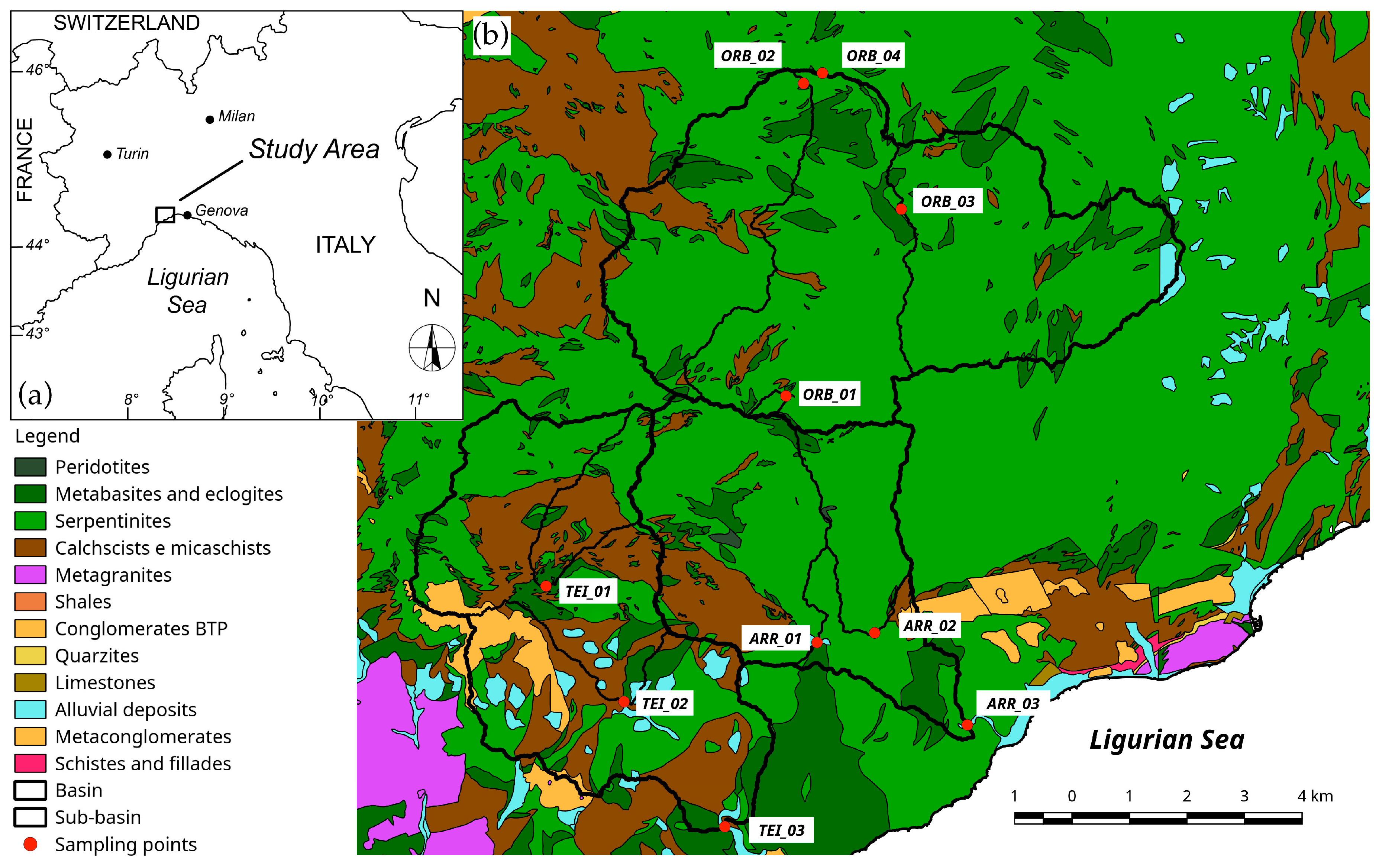
2. Study Area
3. Materials and Methods
3.1. Theoretical Background
3.2. Phases of the Study
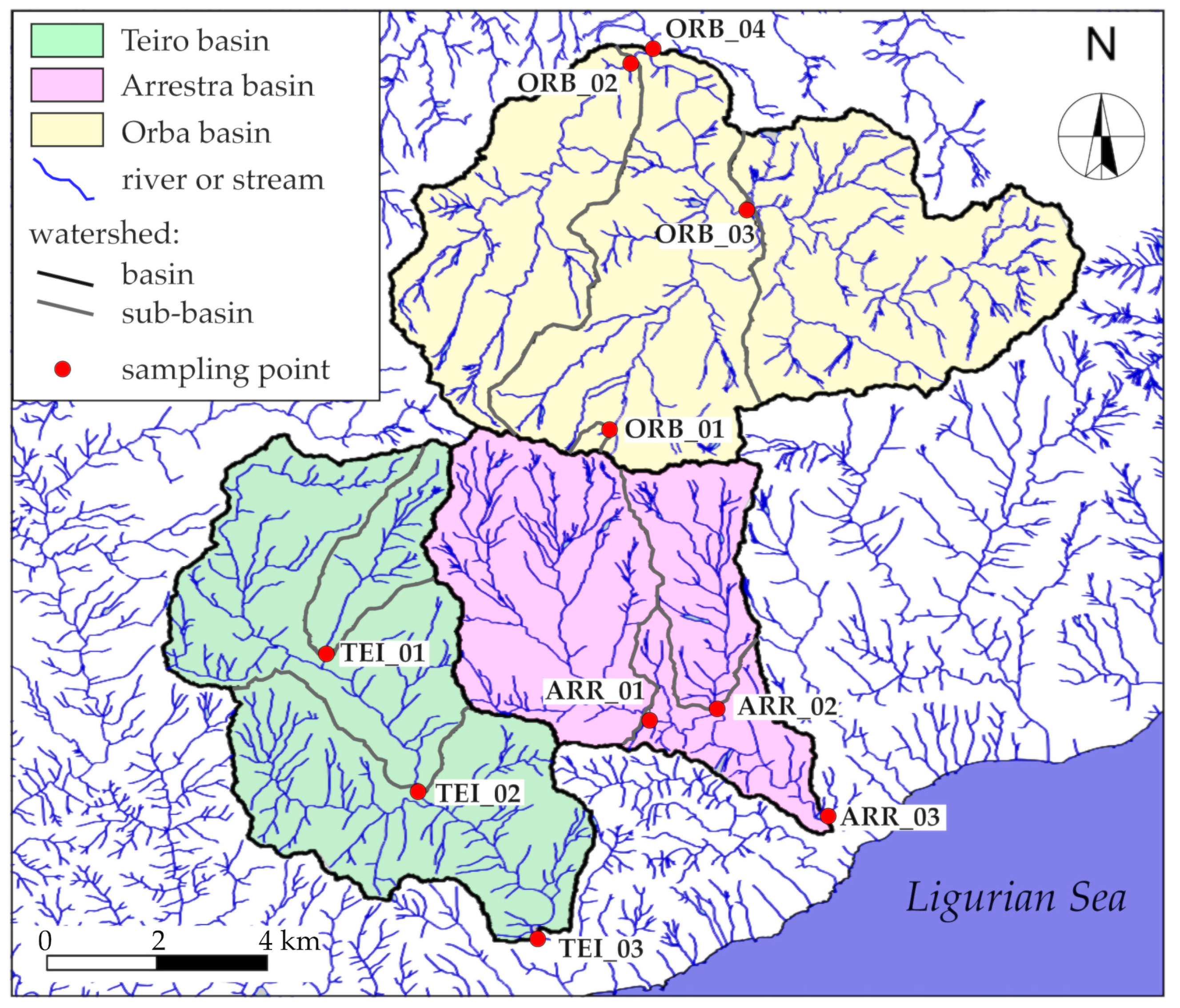
3.3. Definition of the Drainage Basins
3.4. Sampling and Analyses
3.5. Computation of Runoff, Solute Flux, Weathering Rates, and CO2 Consumption Rates
4. Results
4.1. Chemical and Isotopic Composition of Stream Waters
- -
- all the samples are saturated or supersaturated with respect to amorphous Fe(OH)3 and goethite, suggesting that Fe oxyhydroxides control the iron concentration in solution;
- -
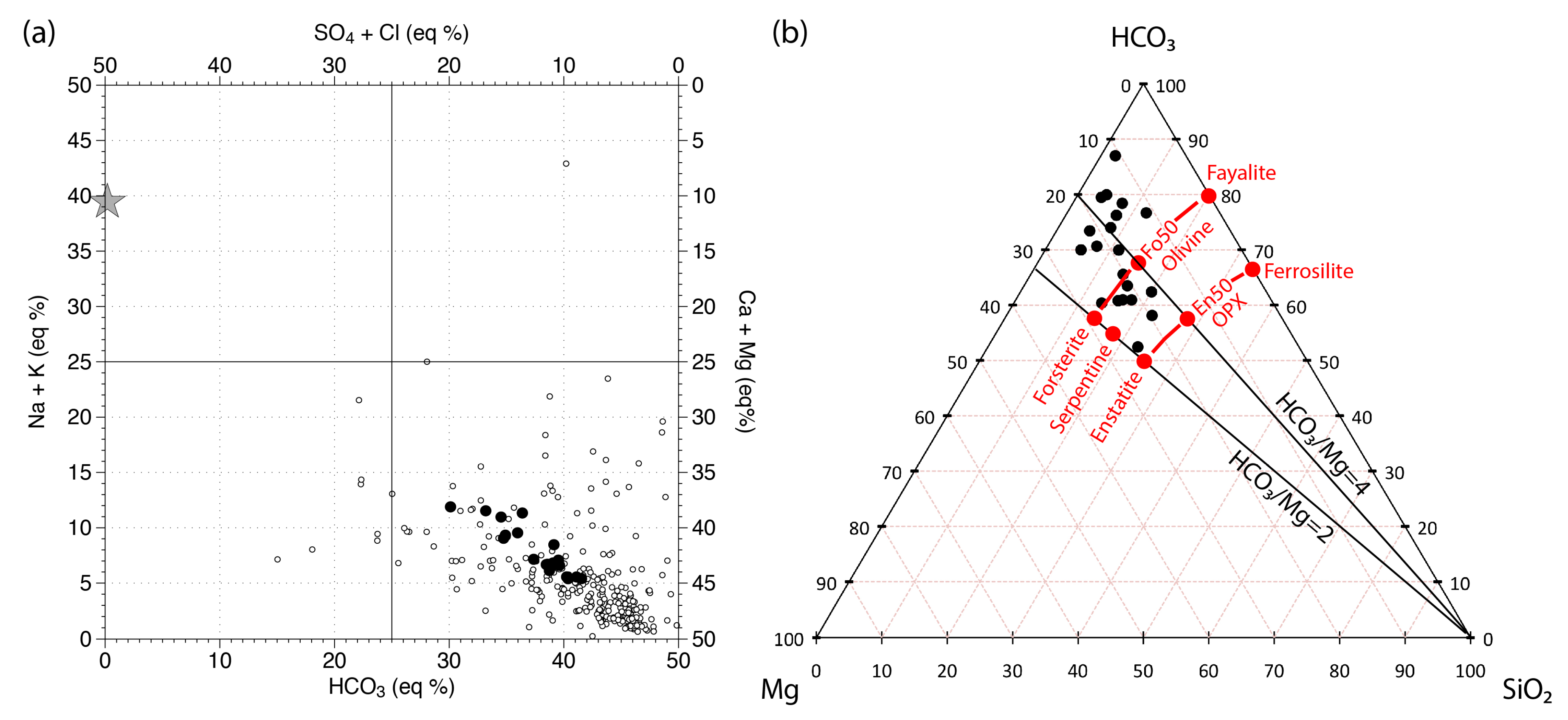
- the samples of the Arrestra and Orba streams are supersaturated with respect to illite, kaolinite, and clay minerals of the smectite group (e.g., montmorillonite), close to equilibrium or supersaturated with respect to gibbsite and quartz (but undersaturated with respect to amorphous silica) and undersaturated with respect to calcite, dolomite, magnesite and brucite;
- -
- the samples of the Teiro stream show extremely variable saturation conditions for clay minerals and quartz, are generally undersaturated with respect to gibbsite, brucite, and magnesite (except for Teiro 3 samples), close to equilibrium or supersaturated with respect to calcite (in particular during the July 2016 survey) and supersaturated with respect to ordered dolomite;
- -
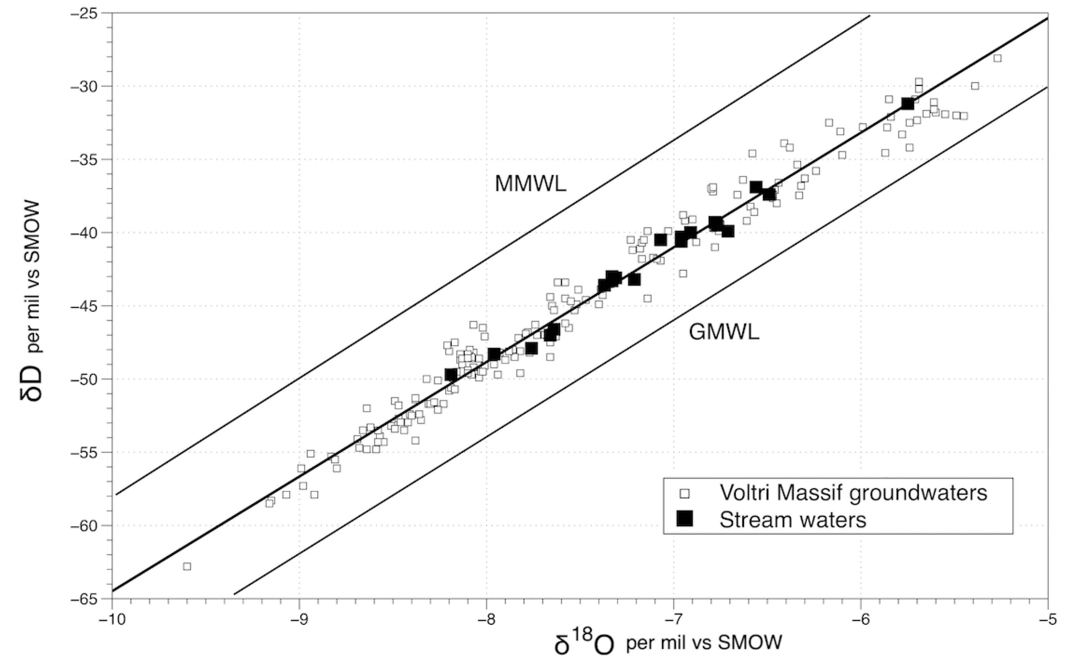
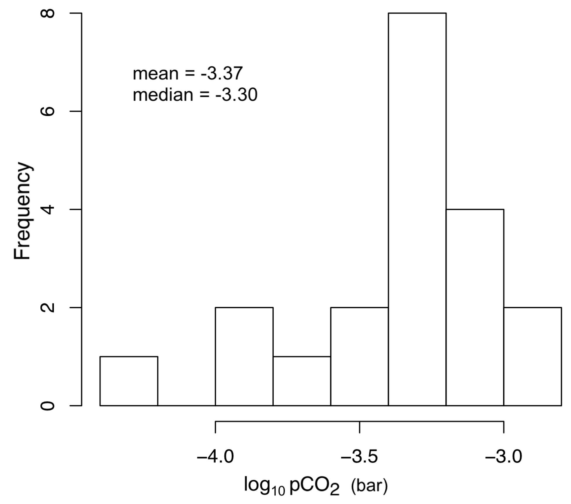
- the logarithm of carbon dioxide partial pressure (log10 pCO2) vary within a relatively small interval, from −4.27 to −2.88, following a log-normal distribution (Figure 5). Its probability distribution is characterized by a mean of −3.37 (10−3.37 bar) and a median of −3.30 (10−3.30 bar), very close to the value of equilibrium with the atmospheric carbon dioxide (10−3.39 bar assuming a CO2 concentration in atmosphere of 405 ppm), and suggests that most of the dissolved inorganic carbon derive from the atmosphere. This hypothesis is supported also by the isotopic composition of TDIC (−14.27 ≤ δ13CTDIC ≤ −6.59) that is consistent with an atmospheric origin (δ13Catm ≈ −8) of dissolved carbon with a minor contribution of soil CO2 deriving from organic matter oxidation (δ13Corg ≈ −28).
4.2. Runoff, Solute Fluxes, Weathering Rates, and CO2 Fluxes
5. Discussion
6. Conclusions
Supplementary Materials
Author Contributions
Funding
Acknowledgments
Conflicts of Interest
References
- Brady, P.V. The effect of silicate weathering on global temperature and atmospheric CO2. J. Geophys. Res. Solid Earth 1991, 96, 18101–18106. [Google Scholar] [CrossRef]
- Kump, L.R.; Arthur, M.A. Global chemical erosion during the Cenozoic: Weatherability balances the budgets. In Tectonic Uplift and Climate Change; Ruddiman, W.F., Ed.; Plenum Press: New York, NY, USA, 1997; pp. 399–426. [Google Scholar]
- Kump, L.R.; Brantley, S.L.; Knoll, M.A. Chemical weathering, atmospheric CO2, and climate. Annu. Rev. Earth Planet. Sci. 2000, 28, 611–667. [Google Scholar] [CrossRef]
- Kump, L.R.; Kasting, J.F.; Crane, R.G. The Earth System, 3rd ed.; Prentice Hall: Upper Saddle River, NJ, USA, 2009; p. 432. [Google Scholar]
- Tipper, E.T.; Bickle, M.J.; Galy, A.; West, A.J.; Pomiès, C.; Chapman, H.J. The short term climatic sensitivity of carbonate and silicate weathering fluxes: Insight from seasonal variations in river chemistry. Geochim. Cosmochim. Acta 2006, 70, 2737–2754. [Google Scholar] [CrossRef]
- White, A.F.; Brantley, S.L. The effect of time on the weathering of silicate minerals: Why do weathering rates differ in the laboratory and field? Chem. Geol. 2003, 202, 479–506. [Google Scholar] [CrossRef]
- Broecker, W.; Yu, J. What do we know about the evolution of Mg to Ca ratios in seawater? Paleoceanography 2011, 26, PA3203. [Google Scholar] [CrossRef]
- Berner, R.A.; Lasaga, A.C.; Garrels, R.M. The carbonate-silicate geochemical cycle and its effect on atmospheric carbon dioxide over the past 100 million years. Am. J. Sci. 1983, 283, 641–683. [Google Scholar] [CrossRef]
- Raymond, P.A.; Oh, N.-H.; Turner, R.E.; Broussard, W. Anthropogenic enhanced fluxes of water and carbon from the Mississippi River. Nature 2008, 451, 449–452. [Google Scholar] [CrossRef] [PubMed]
- Gislason, S.R.; Oelkers, E.H.; Eiriksdottir, E.S.; Kardjilov, M.I.; Gisladottir, G.; Sigfusson, B.; Snorrason, A.; Elefsen, S.; Hardardottir, J.; Torssander, P.; et al. Direct evidence of the feedback between climate and weathering. Earth Planet. Sci. Lett. 2009, 277, 213–222. [Google Scholar] [CrossRef]
- Beaulieu, E.; Goddéris, Y.; Donnadieu, Y.; Labat, D.; Roelandt, C. High sensitivity of the continental-weathering carbon dioxide sink to future climate change. Nat. Clim. Chang. 2012, 2, 346–349. [Google Scholar] [CrossRef]
- Garrels, R.M.; Mackenzie, F.T. Evolution of Sedimentary Rocks; Norton & Co.: New York, NY, USA, 1971; p. 397. [Google Scholar]
- Drever, J.I. The Geochemistry of Natural Waters; Prentice-Hall: Englewood Cliffs, NJ, USA, 1982; p. 388. [Google Scholar]
- Berner, E.K.; Berner, R.A. The Global Water Cycle. Geochemistry and Environment; Prentice Hall: Engelwood Cliffs, NJ, USA, 1987; p. 397. [Google Scholar]
- Probst, J.L.; Mortatti, J.; Tardy, Y. Carbon river fluxes and global weathering CO2 consumption in the Congo and Amazon River Basins. Appl. Geochem. 1994, 9, 1–13. [Google Scholar] [CrossRef]
- Meybeck, M. Global occurrence of major elements in rivers. In Surface and Ground Water, Weathering, and Soils. Treatise on Geochemistry; Drever, J.I., Ed.; Elsevier: Oxford, UK, 2003; Volume 5, pp. 207–224. [Google Scholar]
- Bricker, O.P.; Jones, B.F.; Bowser, C.J. Mass-balance Approach to Interpreting Weathering Reactions in Watershed Systems. In Surface and Ground Water, Weathering, and Soils. Treatise on Geochemistry; Drever, J.I., Ed.; Elsevier: Oxford, UK, 2003; Volume 5, pp. 119–132. [Google Scholar]
- Meybeck, M. Global chemical weathering of surficial rocks estimated from river dissolved load. Am. J. Sci. 1987, 287, 401–428. [Google Scholar] [CrossRef]
- Amiotte-Suchet, P.; Probst, J.L. A global model for present day atmospheric CO2 consumption by chemical erosion of continental rocks (GEM CO2). Tellus 1995, 47, 273–280. [Google Scholar] [CrossRef]
- Boeglin, J.L.; Probst, J.L. Physical and chemical weathering rates and CO2 consumption, in a tropical lateritic environment: The upper Niger basin. Chem. Geol. 1998, 148, 137–156. [Google Scholar] [CrossRef]
- Gaillardet, J.; Dupré, B.; Louvat, P.; Allègre, C.J. Global silicate weathering and CO2 consumption rates deduced from the chemistry of large rivers. Chem. Geol. 1999, 159, 3–30. [Google Scholar] [CrossRef]
- Mortatti, J.; Probst, J.L. Silicate rock weathering and atmospheric/soil CO2 uptake in the Amazon Basin estimated from river water geochemistry: Seasonal and spatial variations. Chem. Geol. 2003, 197, 177–196. [Google Scholar] [CrossRef]
- Donnini, M.; Frondini, F.; Probst, J.L.; Probst, A.; Cardellini, C.; Marchesini, I.; Guzzetti, F. Chemical weathering and consumption of atmospheric carbon dioxide in the Alpine region. Glob. Planet. Chang. 2016, 136, 65–81. [Google Scholar] [CrossRef]
- Amiotte-Suchet, P.; Probst, J.L. Flux de CO2 consommé par altération chimique continentale: Influences du drainage et de la lithologie. C. R. Acad. Sci. Paris II Méc. Phys. Chim. Astron. 1993, 317, 615–622. [Google Scholar]
- Bluth, G.J.S.; Kump, L.R. Lithological and climatological controls of river chemistry. Geochim. Cosmochim. Acta 1994, 58, 2341–2359. [Google Scholar] [CrossRef]
- Gislason, S.R.; Arnorsson, S.; Armansson, H. Chemical weathering of basalt in south-west Iceland: Effects of runoff, age of rocks and vegetative/glacial cover. Am. J. Sci. 1996, 296, 837–907. [Google Scholar] [CrossRef]
- Louvat, P.; Allègre, C.J. Present denudation rates at Réunion Island determined by river geochemistry: Basalt weathering and mass budget between chemical and mechanical erosions. Geochim. Cosmochim. Acta 1997, 61, 3645–3669. [Google Scholar] [CrossRef]
- White, A.F. Natural weathering rates of silicate minerals. In Surface and Ground Water, Weathering, and Soils. Treatise on Geochemistry; Drever, J.I., Ed.; Elsevier: Oxford, UK, 2003; Volume 5, pp. 133–168. [Google Scholar]
- Swoboda-Colberg, N.G.; Drever, J.I. Mineral dissolution rates in plot-scale field and laboratory experiments. Chem. Geol. 1993, 105, 51–69. [Google Scholar] [CrossRef]
- White, A.F.; Brantley, S.L. Chemical weathering rates of silicate minerals: An overview. In Chemical Weathering Rates of Silicate Minerals, Review in Mineralogy; White, A.F., Brantley, S.L., Eds.; Mineralogical Society of America: Chantilly, VA, USA, 1995; Volume 31, pp. 1–22. [Google Scholar]
- Reeves, D.; Rothman, D.H. Age dependence of mineral dissolution and precipitation rates. Glob. Biogeochem. Cycles 2013, 27, 906–919. [Google Scholar] [CrossRef]
- Gruber, C.; Zhu, C.; Georg, R.B.; Zakon, Y.; Ganor, J. Resolving the gap between laboratory and field rates of feldspar weathering. Geochim. Cosmochim. Acta 2014, 147, 90–106. [Google Scholar] [CrossRef]
- Berner, R.A. The long-term carbon cycle, fossil fuels and atmospheric composition. Nature 2003, 426, 323–326. [Google Scholar] [CrossRef] [PubMed]
- Beinlich, A.; Austrheim, H.; Mavromatis, V.; Grguric, B.; Putnis, C.V.; Putnis, A. Peridotite weathering is the missing ingredient of Earth’s continental crust composition. Nat. Commun. 2018, 9, 634. [Google Scholar] [CrossRef]
- Cipolli, F.; Gambardella, B.; Marini, L.; Ottonello, G.; Vetuschi Zuccolini, M. Geochemistry of high-pH waters from serpentinites of the Gruppo di Voltri (Genova, Italy) and reaction path modeling of CO2 sequestration in serpentinite aquifers. Appl. Geochem. 2004, 19, 787–802. [Google Scholar] [CrossRef]
- Marini, L. Geological Sequestration of Carbon Dioxide: Thermodynamics, Kinetics, and Reaction Path Modeling; Developments in Geochemistry 11; Elsevier: Oxford, UK, 2007; p. 453. [Google Scholar]
- Kelemen, P.B.; Matter, J. In situ carbonation of peridotite for CO2 storage. Proc. Natl. Acad. Sci. USA 2008, 105, 17295–17300. [Google Scholar] [CrossRef]
- Regione Liguria. Geoportale, Litologia and CARG maps. Available online: https://geoportal.regione.liguria.it/mappe (accessed on 5 February 2019).
- Capponi, G.; Crispini, L.; Federico, L.; Malatesta, C. Geology of the Eastern Ligurian Alps: A review of the tectonic units. Ital. J. Geosci. 2016, 135, 157–169. [Google Scholar] [CrossRef]
- Gelati, R.; Gnaccolini, M. Synsedimentary tectonics and sedimentation in the Tertiary Piedmont Basin, Northwestern Italy. Riv. It. Paleont. Strat. 1998, 104, 193–214. [Google Scholar]
- Mutti, E.; Papani, L.; Di Biase, D.; Davoli, G.; Mora, S.; Segadelli, S.; Tinterri, R. Il Bacino Terziario Epimesoalpino e le sue implicazioni sui rapporti tra Alpi e Appennino. Memorie Scienze Geologiche 1995, 47, 217–244. [Google Scholar]
- Maino, M.; Decarlis, A.; Felletti, F.; Seno, S. Tectono-sedimentary evolution of the Tertiary Piedmont Basin (NW Italy) within the Oligo–Miocene central Mediterranean geodynamics. Tectonics 2013, 2, 593–619. [Google Scholar] [CrossRef]
- Federico, L.; Crispini, L.; Malatesta, C.; Torchio, S.; Capponi, G. Geology of the Pontinvrea area (Ligurian Alps, Italy): Structural setting of the contact between Montenotte and Voltri units. J. Maps 2015, 11, 101–113. [Google Scholar] [CrossRef]
- Vanossi, M.; Cortesogno, L.; Galbiati, B.; Messiga, B.; Piccardo, G.; Vannucci, R. Geologia delle Alpi Liguri: Dati, problemi, ipotesi. Mem. Soc. Geol. Ital. 1986, 28, 5–75. [Google Scholar]
- Chiesa, S.; Cortesogno, L.; Forcella, F.; Galli, M.; Messiga, B.; Pasquare, G.; Pedemonte, G.M.; Piccardo, G.B. Assetto strutturale ed interpretazione geodinamica del Gruppo di Voltri. Bol. Soc. Geol. It. 1975, 94, 555–581. [Google Scholar]
- Treble, P.J. The Voltri Group, Northern Italy: An Alpine ophiolite massif. In Evolution of Metamorphic Belts; Daly, J.S., Cliff, R.A., Yardley, B.W.D., Eds.; Geological Society: London, UK, 1989; Volume 43, pp. 551–556. [Google Scholar]
- Stampfli, G.M.; Vavassis, I.; De Bono, A.; Rosselet, F.; Matti, B.; Bellini, M. Remnants of the Paleotethys oceanic suture-zone in the western Tethyan area. Bol. Soc. Geol. It. 2003, 2, 1–23. [Google Scholar]
- Piccardo, G.B. The Jurassic Ligurian Tethys, a fossil ultraslow-spreading ocean: The mantle perspective. In Metasomatism in Oceanic and Continental Lithospheric Mantle; Coltorti, M., Grégoire, M., Eds.; Geological Society: London, UK, 2008; Volume 293, pp. 11–34. [Google Scholar]
- Piccardo, G.B.; Padovano, M.; Guarnieri, L. The Ligurian Tethys: Mantle processes and geodynamics. Earth-Sci. Rev. 2014, 138, 409–434. [Google Scholar] [CrossRef]
- Piccardo, G.B. Le ofioliti dell’areale ligure: Petrologia e ambiente geodinamico di formazione (relazione ufficiale). Ofioliti 1976, 1, 469–500. [Google Scholar]
- Piccardo, G.B. Le ofioliti metamorfiche del Gruppo di Voltri, Alpi Liguri: Caratteri primari e interpretazione geodinamica. Mem. Soc. Geol. It. 1984, 28, 95–114. [Google Scholar]
- Messiga, B.; Scambelluri, M. Retrograde P-T-t path for the Voltri Massif eclogites (Ligurian Alps, Italy): Some tectonic implications. J. Metamorph. Geol. 1991, 9, 93–109. [Google Scholar] [CrossRef]
- Crispini, L.; Capponi, G. Tectonic evolution of the Voltri Group and Sestri Voltaggio zone (southern limit of the NW Alps): A review. Ofioliti 2001, 26, 161–164. [Google Scholar]
- Vignaroli, G.; Rossetti, F.; Rubatto, D.; Theye, T.; Lisker, F.; Phillips, D. Pressure-temperature-deformation-time (P-T-d-t) exhumation history of the Voltri Massif HP complex, Ligurian Alps, Italy. Tectonics 2010, 29, TC6009. [Google Scholar] [CrossRef]
- Seno, S.; Dallagiovanna, G.; Vanossi, M. A kinematic evolution model for the Penninic sector of the central Ligurian Alps. Int. J. Earth Sci. 2005, 94, 114–129. [Google Scholar] [CrossRef]
- Capponi, G.; Crispini, L. Structural and metamorphic signature of Alpine tectonics in the Voltri Massif (Ligurian Alps, northwestern Italy). Ecl. Geol. Helv. 2002, 95, 31–42. [Google Scholar]
- Federico, L.; Capponi, G.; Crispini, L.; Scambelluri, M.; Villa, I.M. 39Ar/40Ar dating of high pressure rocks from the Ligurian Alps: Evidence for a continuous subduction–exhumation cycle. Earth Planet. Sci. Lett. 2005, 240, 668–680. [Google Scholar] [CrossRef]
- Speranza, F.; Villa, I.M.; Sagnotti, L.; Florindo, F.; Cosentino, D.; Cipollari, P.; Mattei, M. Age of the Corsica–Sardinia rotation and Liguro–Provençal Basin spreading: New paleomagnetic and Ar/Ar evidence. Tectonophysics 2002, 347, 231–251. [Google Scholar] [CrossRef]
- Gattacceca, J.; Deino, A.; Rizzo, R.; Jones, D.S.; Henry, B.; Beaudoin, B.; Vadeboin, F. Miocene rotation of Sardinia: New paleomagnetic and geochronological constraints and geodynamic implications. Earth Planet. Sci. Lett. 2007, 258, 359–377. [Google Scholar] [CrossRef]
- Firpo, M.; Piccazzo, M. Geomofologia. In Note Illustrative Della Carta Geologica d’Italia, Foglio 213–230 Genova; Capponi, G., Crispini, L., Eds.; APAT Servizio Geologico d’Italia: Ispra, Italy, 2013; pp. 99–106. [Google Scholar]
- ARPAL. Atlante Climatico della Liguria; ARPAL: Genova, Italy, 2013; p. 128. [Google Scholar]
- Bocchio, R. Chemical variations in clinopyroxenes and garnet from eclogites of the Vara Valley (Voltri Group), Italy. Eur. J. Mineral. 1995, 7, 103–117. [Google Scholar] [CrossRef]
- Regione Liguria. Geoportale, DTM—Modello Digitale del Terreno—Liguria 2016. Available online: https://geoportal.regione.liguria.it (accessed on 15 December 2018).
- Neteler, M.; Bowman, M.H.; Landa, M.; Metz, M. GRASS GIS: A multi-purpose open source GIS. Environ. Model. Softw. 2012, 31, 124–130. [Google Scholar] [CrossRef]
- Amiotte-Suchet, P.; Probst, J.L. Modelling of atmospheric CO2 consumption by chemical weathering of rocks: Application to the Garonne, Congo and amazon basins. Chem. Geol. 1993, 107, 205–210. [Google Scholar] [CrossRef]
- Ladouche, B.; Aquilina, L.; Dörfliger, N. Chemical and isotopic investigation of rainwater in Southern France (1996–2002): Potential use as input signal for karst functioning investigation. J. Hydrol. 2009, 367, 150–164. [Google Scholar] [CrossRef]
- Celle, H. Caractérisation des Précipitations sur le Pourtour de la Méditerranée Occidentale–Approche Isotopique et Chimique. Ph.D. Thesis, University of Avignon, Avignon, France, 2000. [Google Scholar]
- Craig, H. Isotopic variations in meteoric waters. Science 1961, 133, 1702–1703. [Google Scholar] [CrossRef] [PubMed]
- Longinelli, A.; Selmo, E. Isotopic composition of precipitation in Italy: A first overallmap. J. Hydrol. 2003, 270, 75–88. [Google Scholar]
- Marini, L.; Ottonello, G. (Eds.) Atlante Degli Acquiferi Della Liguria-Vol. III: Le Acque Dei Complessi Ofiolitici (Bacini Arrestra, Branega, Cassinelle, Cerusa, Erro, Gorzente, Leira, Lemme, Lerone, Orba, Piota, Polcevera, Rumaro, Sansobbia, Stura, Teiro, Varenna, Visone); Pacini Editore: Pisa, Italy, 2002. [Google Scholar]
- Parkhurst, D.L. User’s Guide to PHREEQC: A Computer Program. for Speciation, Reaction-Path, Advective-Transport., and Inverse Geochemical Calculations; Water-Resources Investigations Report 95-4227; U.S. Geological Survey, Earth Science Information Center, Open-File Reports Section: Lakewood, CO, USA, 1995; p. 143. [Google Scholar]
- Wolery, T.J. Calculation of Chemical Equilibrium between Aqueous Solution and Minerals-The EQ3/6 Software Package; Lawrence Livermore National Laboratory Report UCRL-52658; Lawrence Livermore National Laboratory: Livermore, CA, USA, 1979; p. 41. [Google Scholar]
- Bonifacio, E.; Zanini, E.; Boero, V.; Franchini-Angela, M. Pedogenesis in a soil catena on serpentinite in north-western Italy. Geoderma 1997, 75, 33–51. [Google Scholar] [CrossRef]
- Reeder, R.J.; Nakajima, Y. The nature of ordering and ordering defects in dolomite. Phys. Chem. Miner. 1982, 8, 29–35. [Google Scholar] [CrossRef]
- Zucchini, A.; Comodi, P.; Katerinopoulou, A.; Balic-Zunic, T.; McCammon, C.; Frondini, F. Order-disorder-reorder process in thermally treated dolomite samples: A combined powder and single-crystal X-ray diffraction study. Phys. Chem. Miner. 2012, 39, 319–328. [Google Scholar] [CrossRef]
- Arvidson, R.S.; Mackenzie, F.T. The dolomite problem: Control of precipitation kinetics by temperature and saturation state. Am. J. Sci. 1999, 299, 257–288. [Google Scholar] [CrossRef]
- Power, I.M.; Wilson, S.A.; Dipple, G.M. Serpentinite Carbonation for CO2 Sequestration. Elements 2013, 9, 115–121. [Google Scholar] [CrossRef]
- Ulven, O.; Beinlich, A.; Hövelmann, J.; Austrheim, H.; Jamtveit, B. Subarctic physicochemical weathering of serpentinized peridotite. Earth Planet. Sci. Lett. 2017, 468, 11–26. [Google Scholar] [CrossRef]
- Piccardo, G.B.; Rampone, E.; Romairone, A.; Scambelluri, M.; Tribuzio, R.; Beretta, C. Evolution of the Ligurian Tethys: Inference from petrology and geochemistry of the Ligurian Ophiolites. Per. Mineral. 2001, 70, 147–192. [Google Scholar]
- Boulart, C.; Chavagnac, V.; Monnin, C.; Delacour, A.; Ceuleneer, G.; Hoareau, G. Differences in gas venting from ultramafic-hosted warm springs: The example of Oman and Voltri Ophiolites. Ofioliti 2013, 38, 143–156. [Google Scholar]
- Hartmann, J.; Jansen, N.; Dürr, H.H.; Kempe, S.; Köhler, P. Global CO2-consumption by chemical weathering: What is the contribution of highly active weathering regions? Glob. Planet. Chang. 2009, 69, 185–194. [Google Scholar] [CrossRef]
- Hartmann, J.; Moosdorf, N. The new global lithological map database GLiM: A representation of rock properties at the Earth surface. Geochem. Geophys. Geosyst. 2012, 13, Q12004. [Google Scholar] [CrossRef]
- Schopka, H.H.; Derry, L.A.; Arcilla, C.A. Chemical weathering, river geochemistry and atmospheric carbon fluxes from volcanic and ultramafic regions on Luzon Island, the Philippines. Geochim. Cosmochim. Acta 2011, 75, 978–1002. [Google Scholar] [CrossRef]
- Pearson, K. Notes on regression and inheritancein the case of two parents. Proc. R. Soc. Lond. 1895, 58, 240–242. [Google Scholar]
- Wessa, P. Multivariate Correlation Matrix (v1.0.11) in Free Statistics Software (v1.2.1), Office for Research Development and Education. 2016. Available online: http://www.wessa.net/Patrick.Wessa/rwasp_pairs.wasp/ (accessed on 2 April 2019).
- Guo, S.; Wang, J.; Xiong, L.; Ying, A.; Li, D. A macro-scale and semi-distributed monthly water balance model to predict climate change impacts in China. J. Hydrol. 2002, 268, 1–15. [Google Scholar] [CrossRef]
- Legesse, D.; Vallet-Coulomb, C.; Gasse, F. Hydrological response of a catchment to climate and land use changes in Tropical Africa: Case study South Central Ethiopia. J. Hydrol. 2003, 275, 67–85. [Google Scholar] [CrossRef]
- Jiang, T.; Chen, J.D.; Xu, C.; Chen, X.; Chen, X.; Singh, V.P. Comparison of hydrological impacts of climate change simulated by six hydrological models in the Dongjiang Basin, South China. J. Hydrol. 2007, 336, 316–333. [Google Scholar] [CrossRef]
- Lin, Y.; Wen, H.; Liu, S. Surface runoff response to climate change based on artificial neural network (ANN) models: A case study with Zagunao catchment in Upper Minjiang River, Southwest China. J. Water Clim. Chang. 2019, 10, 158–166. [Google Scholar] [CrossRef]
- Strefler, J.; Amann, T.; Bauer, N.; Kriegler, E.; Hartmann, J. Potential and costs of carbon dioxide removal by enhanced weathering of rocks. Environ. Res. Lett. 2018, 13, 034010. [Google Scholar] [CrossRef]
- Dilek, Y.; Robinson, P.T. (Eds.) Ophiolites in Earth History; Geological Society Special Publication 218; Geological Society of London: London, UK, 2003; p. 723. [Google Scholar]


| Drainage Basin | Sub-Basin 1 | Surface (km2) | Mean Elevation (m a.s.l) | Minimum Elevation (m a.s.l) | Maximum Elevation (m a.s.l) |
|---|---|---|---|---|---|
| Teiro | Teiro 1 | 2.9 | 843 | 370 | 1287 |
| Teiro | Teiro 2 | 14.6 | 665 | 100 | 1287 |
| Teiro | Teiro 3 | 26.5 | 487 | 10 | 1287 |
| Arrestra | Arrestra 1 | 11.7 | 741 | 171 | 1287 |
| Arrestra | Arrestra 2 | 4.7 | 677 | 139 | 1145 |
| Arrestra | Arrestra 3 | 20.0 | 632 | 20 | 1287 |
| Orba | Orba 1 | 0.2 | 1137 | 1081 | 1198 |
| Orba | Orba 2 | 10.7 | 939 | 730 | 1287 |
| Orba | Orba 3 | 14.6 | 915 | 610 | 1181 |
| Orba | Orba 4 | 39.6 | 919 | 540 | 1287 |
| Sub-Basin | Peridotites | Metabasites * | Serpentinite | Calc-Schistes | Conglomerates |
|---|---|---|---|---|---|
| Teiro 1 | 0.0 | 10.3 | 41.4 | 48.3 | 0.0 |
| Teiro 2 | 0.0 | 12.4 | 47.6 | 36.6 | 3.4 |
| Teiro 3 | 0.0 | 14.0 | 43.4 | 36.2 | 6.4 |
| Arrestra 1 | 0.9 | 10.3 | 63.9 | 24.8 | 0.0 |
| Arrestra 2 | 0.0 | 4.3 | 93.6 | 2.1 | 0.0 |
| Arrestra 3 | 0.5 | 12.5 | 71.8 | 14.9 | 0.0 |
| Orba 1 | 0.0 | 0.0 | 100.0 | 0.0 | 0.0 |
| Orba 2 | 0.0 | 12.1 | 78.5 | 9.3 | 0.0 |
| Orba 3 | 0.0 | 13.7 | 84.2 | 2.1 | 0.0 |
| Orba 4 | 0.0 | 13.4 | 81.6 | 5.1 | 0.0 |
| ID | Log10 pCO2 | Caclite. | Dol. ord. | Dol. dis. | Magn. | Brucite | Gibbsite | Qz | SiO2 am. | Montm. | Kaol. | Illite | Goeth. | Fe(OH)3 |
|---|---|---|---|---|---|---|---|---|---|---|---|---|---|---|
| July 2016 | ||||||||||||||
| Arr. 1 | −2.88 | −0.34 | 0.36 | −1.39 | −0.94 | −4.35 | 0.27 | 0.25 | −1.05 | 1.94 | 1.74 | 1.09 | nc | nc |
| Arr. 2 | −3.14 | −0.96 | −0.44 | −2.02 | −1.14 | −4.37 | 0.00 | 0.47 | −0.84 | 2.35 | 1.63 | 1.06 | nc | nc |
| Arr. 3 | −3.18 | −0.21 | 0.88 | −0.67 | −0.55 | −3.60 | 0.22 | 0.52 | −0.77 | 3.30 | 2.18 | 2.30 | 6.43 | 0.58 |
| Teiro 1 | −3.43 | 0.06 | 0.77 | −0.83 | −0.97 | −4.05 | −0.29 | −0.32 | −1.66 | −1.14 | −0.55 | −1.90 | nc | nc |
| Teiro 2 | −3.40 | 0.34 | 1.52 | −0.03 | −0.46 | −3.30 | nc | 0.22 | −1.08 | nc | Nc | nc | nc | nc |
| Teiro 3 | −3.92 | 1.10 | 3.39 | 1.67 | 0.48 | −1.69 | −0.98 | 0.20 | −1.05 | 1.04 | −0.82 | −0.33 | 6.34 | 0.38 |
| Orba 1 | −3.26 | −1.89 | −2.60 | −4.22 | −2.41 | −5.83 | nc | 0.37 | −1.00 | nc | Nc | nc | 6.96 | 1.48 |
| Orba 2 | −3.23 | −1.23 | −1.10 | −2.70 | −1.55 | −4.84 | 0.51 | 0.48 | −0.87 | 2.96 | 2.62 | 1.97 | 6.58 | 0.95 |
| Orba 3 | −3.31 | −1.60 | −1.65 | −3.26 | −1.73 | −4.95 | 0.25 | 0.25 | −1.10 | 1.55 | 1.64 | 0.73 | nc | nc |
| Orba 4 | −3.11 | −1.23 | −1.13 | −2.72 | −1.57 | −4.91 | 0.21 | 0.41 | −0.92 | 2.18 | 1.91 | 1.13 | 6.54 | 0.87 |
| April 2017 | ||||||||||||||
| Arr. 1 | −3.29 | −0.80 | −0.57 | −2.21 | −1.48 | −5.01 | 0.36 | 0.48 | −0.92 | 2.60 | 2.27 | 1.59 | nc | nc |
| Arr. 2 | −3.31 | −1.08 | −0.78 | −2.42 | −1.41 | −4.90 | 0.35 | 0.64 | −0.75 | 3.31 | 2.59 | 1.98 | 6.70 | 1.29 |
| Arr. 3 | −2.98 | −1.09 | −0.99 | −2.64 | −1.62 | −5.43 | 0.60 | 0.33 | −1.07 | 2.18 | 2.44 | 1.43 | 6.69 | 1.27 |
| Teiro 1 | −3.62 | −0.27 | 0.11 | −1.54 | −1.34 | −4.60 | 0.56 | 0.53 | −0.88 | 3.33 | 2.76 | 2.70 | nc | nc |
| Teiro 2 | −3.84 | −0.17 | 0.51 | −1.13 | −1.03 | −4.00 | −0.18 | −0.06 | −1.45 | 0.05 | 0.12 | −0.77 | nc | nc |
| Teiro 3 | −4.27 | 0.94 | 2.75 | 1.13 | 0.11 | −2.33 | −0.95 | 0.17 | −1.21 | 0.53 | −0.94 | −0.82 | nc | nc |
| Orba 1 | −3.39 | −1.68 | −2.69 | −4.37 | −2.75 | −6.33 | 0.80 | −1.57 | −0.14 | 0.17 | 1.88 | 0.00 | nc | nc |
| Orba 2 | −3.17 | −1.85 | −2.48 | −4.14 | −2.36 | −6.10 | 1.12 | 0.63 | −0.78 | 3.95 | 4.09 | 3.04 | 7.06 | 1.74 |
| Orba 3 | −3.23 | −1.80 | −2.33 | −3.99 | −2.25 | −5.91 | 1.44 | −0.20 | −1.61 | 1.25 | 3.07 | 1.20 | nc | nc |
| Orba 4 | −3.39 | −2.29 | −3.06 | −4.72 | −2.50 | −6.02 | 1.08 | 0.51 | −0.90 | 3.43 | 3.76 | 2.89 | 6.76 | 1.43 |
| Basin/Sub-Basin | Runoff | Solute Flux | Weathering Rate | FCO2-Short | FCO2-Long | ||
|---|---|---|---|---|---|---|---|
| L s−1 km−2 | t km−2 y−1 | t km−2 y−1 | mol km−2 y−1 | t km−2 y−1 | mol km−2 y−1 | t km−2 y−1 | |
| July 2016 | |||||||
| Arrestra | |||||||
| Arrestra 1 | 1.7 | 8.1 | 2.9 | 5.96 × 10⁵ | 2.6 | 2.25 × 10⁴ | 1.0 |
| Arrestra 2 | 21.3 | 66.0 | 19.5 | 5.44 × 10⁵ | 24.0 | 2.72 × 10⁵ | 12.0 |
| Arrestra 3 | 8.3 | 79.9 | 30.3 | 5.84 × 10⁵ | 25.7 | 2.30 × 10⁵ | 10.1 |
| weighted mean | 7.5 | 34.6 | 11.8 | 2.68 × 10⁵ | 11.8 | 1.19 × 10⁵ | 5.2 |
| Teiro | |||||||
| Teiro 1 | 15.5 | 61.5 | 27.0 | 3.84 × 10⁵ | 16.9 | 8.53 × 10⁴ | 3.8 |
| Teiro 2 | 2.1 | 15.1 | 5.5 | 9.56 × 10⁴ | 4.2 | 3.55 × 10⁴ | 1.6 |
| Teiro 3 | 10.9 | 82.8 | 31.3 | 5.35 × 10⁵ | 23.5 | 1.85 × 10⁵ | 8.1 |
| weighted mean | 7.5 | 48.6 | 18.9 | 3.24 × 10⁵ | 14.3 | 1.08 × 10⁵ | 4.8 |
| Orba | |||||||
| Orba 1 | 15.0 | 23.7 | 8.5 | 1.51 × 10⁵ | 6.6 | 6.02 × 10⁴ | 2.6 |
| Orba 2 | 7.0 | 17.2 | 5.4 | 1.28 × 10⁵ | 5.6 | 6.10 × 10⁴ | 2.7 |
| Orba 3 | 6.8 | 13.7 | 3.9 | 1.15 × 10⁵ | 5.1 | 5.55 × 10⁴ | 2.4 |
| Orba 4 | 6.5 | 22.5 | 5.2 | 1.23 × 10⁵ | 5.4 | 5.84 × 10⁴ | 2.6 |
| weighted mean | 6.8 | 17.7 | 4.8 | 1.22 × 10⁵ | 5.4 | 5.81 × 10⁴ | 2.6 |
| April 2017 | |||||||
| Arrestra | |||||||
| Arrestra 1 | 17.1 | 54.2 | 17.1 | 3.38 × 10⁵ | 14.9 | 1.42 × 10⁵ | 6.3 |
| Arrestra 2 | 42.6 | 125 | 40.0 | 9.45 × 10⁵ | 41.6 | 4.71 × 10⁵ | 20.7 |
| Arrestra 3 | 27.8 | 11.9 | 18.3 | 1.12 × 10⁶ | 49.4 | 4.18 × 10⁵ | 18.4 |
| weighted mean | 25.0 | 81.2 | 22.0 | 5.91 × 10⁵ | 26.0 | 2.69 × 10⁵ | 11.8 |
| Teiro | |||||||
| Teiro 1 | 51.7 | 174.5 | 74.9 | 9.37 × 10⁵ | 41.2 | 2.45 × 10⁵ | 10.6 |
| Teiro 2 | 4.3 | 11.1 | 1.0 | 8.35 × 10⁴ | 3.7 | 4.17 × 10⁴ | 1.8 |
| Teiro 3 | 6.7 | 67.4 | 21.1 | 4.97 × 10⁵ | 21.9 | 1.56 × 10⁵ | 6.8 |
| weighted mean | 10.6 | 55.3 | 19.8 | 3.48 × 10⁵ | 15.3 | 1.15 × 10⁵ | 5.0 |
| Orba | |||||||
| Orba 1 | 50.0 | 73.0 | 19.15 | 4.90 × 10⁵ | 21.5 | 2.04 × 10⁵ | 9.0 |
| Orba 2 | 18.7 | 37.2 | 11.9 | 2.16 × 10⁵ | 9.5 | 1.06 × 10⁵ | 4.6 |
| Orba 3 | 13.7 | 24.3 | 5.0 | 1.62 × 10⁵ | 7.1 | 7.80 × 10⁴ | 3.4 |
| Orba 4 | 13.5 | 11.4 | 8.8 | 1.13 × 10⁵ | 5 | 5.66 × 10⁴ | 2.5 |
| weighted mean | 15.5 | 23.6 | 8.4 | 1.62 × 10⁵ | 7.1 | 8.03 × 10⁴ | 3.5 |
| FCO2-Short | FCO2-Long | Weathering Rate | Runoff | Temperature | Flow Rate | Altitude | |
|---|---|---|---|---|---|---|---|
| FCO2-short | 1.000 | 0.938 | 0.762 | 0.707 | −0.140 | 0.247 | −0.561 |
| FCO2-long | 1.000 | 0.588 | 0.674 | −0.145 | 0.251 | −0.512 | |
| Weathering Rate | 1.000 | 0.694 | −0.067 | −0.008 | −0.358 | ||
| Runoff | 1.000 | −0.541 | −0.002 | 0.094 | |||
| Temperature | 1.000 | −0.308 | −0.398 | ||||
| Flow rate | 1.000 | −0.305 | |||||
| Altitude | 1.000 |
© 2019 by the authors. Licensee MDPI, Basel, Switzerland. This article is an open access article distributed under the terms and conditions of the Creative Commons Attribution (CC BY) license (http://creativecommons.org/licenses/by/4.0/).
Share and Cite
Frondini, F.; Vaselli, O.; Vetuschi Zuccolini, M. Consumption of Atmospheric Carbon Dioxide through Weathering of Ultramafic Rocks in the Voltri Massif (Italy): Quantification of the Process and Global Implications. Geosciences 2019, 9, 258. https://doi.org/10.3390/geosciences9060258
Frondini F, Vaselli O, Vetuschi Zuccolini M. Consumption of Atmospheric Carbon Dioxide through Weathering of Ultramafic Rocks in the Voltri Massif (Italy): Quantification of the Process and Global Implications. Geosciences. 2019; 9(6):258. https://doi.org/10.3390/geosciences9060258
Chicago/Turabian StyleFrondini, Francesco, Orlando Vaselli, and Marino Vetuschi Zuccolini. 2019. "Consumption of Atmospheric Carbon Dioxide through Weathering of Ultramafic Rocks in the Voltri Massif (Italy): Quantification of the Process and Global Implications" Geosciences 9, no. 6: 258. https://doi.org/10.3390/geosciences9060258
APA StyleFrondini, F., Vaselli, O., & Vetuschi Zuccolini, M. (2019). Consumption of Atmospheric Carbon Dioxide through Weathering of Ultramafic Rocks in the Voltri Massif (Italy): Quantification of the Process and Global Implications. Geosciences, 9(6), 258. https://doi.org/10.3390/geosciences9060258