Article

New Sensitivity Indices of a 2D Flood Inundation Model Using Gauss Quadrature Sampling

1
Centre Eau Terre Environnement, Québec, QC G1K 9A9, Canada
2
Geological Survey of Canada, Quebec, QC G1K 9A9, Canada
*
Author to whom correspondence should be addressed.
Geosciences 2019, 9(5), 220; https://doi.org/10.3390/geosciences9050220
Submission received: 15 March 2019 / Revised: 26 April 2019 / Accepted: 11 May 2019 / Published: 14 May 2019
(This article belongs to the Special Issue Impacts of Compound Hydrological Hazards or Extremes)

Abstract

:
A new method for sensitivity analysis of water depths is presented based on a two-dimensional hydraulic model as a convenient and cost-effective alternative to Monte Carlo simulations. The method involves perturbation of the probability distribution of input variables. A relative sensitivity index is calculated for each variable, using the Gauss quadrature sampling, thus limiting the number of runs of the hydraulic model. The variable-related highest variation of the expected water depths is considered to be the most influential. The proposed method proved particularly efficient, requiring less information to describe model inputs and fewer model executions to calculate the sensitivity index. It was tested over a 45 km long reach of the Richelieu River, Canada. A 2D hydraulic model was used to solve the shallow water equations (SWE). Three input variables were considered: Flow rate, Manning’s coefficient, and topography of a shoal within the considered reach. Four flow scenarios were simulated with discharge rates of 759, 824, 936, and 1113 m 3 / s . The results show that the predicted water depths were most sensitive to the topography of the shoal, whereas the sensitivity indices of Manning’s coefficient and the flow rate were comparatively lower. These results are important for making better hydraulic models, taking into account the sensitivity analysis.

1. Introduction

Hydraulic models provide essential hydraulic parameters for informed flood risk management, such as water depths, velocities, and timing of inundation. The hydraulic models include one-dimensional (1D), two dimensional (2D), and three-dimensional (3D) methodologies that simulate water movement by solving equations derived from applying physical laws to fluid motion with varying degrees of complexity. Different physical processes may be governing at different spatial scales. For instance, although 1D hydraulic may be appropriate for large-scale or even global applications, explicitly modelling floodplain flow with 1D/2D models can be vital for more local assessments. Parallel computing techniques, such as graphics processing unit (GPU) high-performance computing, have been reported to substantially accelerate simplified or full hydraulic/hydrodynamic models for large-scale flood modelling (e.g., [1,2,3,4,5]). As other numerical models, they represent an approximation of physical phenomena and may be affected by various sources of errors, i.e., uncertainties in input data, model structure, and model parameters [6,7]. Knowledge of uncertainties introduced by the model is important for many research questions and is essential in improving simulation performance and increasing confidence in results [8]. A spatially distributed sensitivity analysis (SA) is generally applied to investigate the relative influence of the input variables (individual or in combination) and their impacts on the model outputs [9,10]. Methods such as the Monte Carlo analysis have been applied successfully in a wide range of studies, like flood inundation modelling [11,12]. To take into account the non-linear aspects of the hydrodynamic model, the traditional Monte Carlo method takes into account the complete probability distribution of the input variables and their correlations as key parameters to provide the probability distribution function (PDF) of the output. It is from the input PDFs that the repeated random sampling is employed to evaluate uncertainty and sensitivity in the model results. In addition, this type of analyses allows for accounting of any model, ignoring structures in the input data and assessment of their impacts on results, such as misspecification of respective PDFs and existence of heterogeneity. Sensitivity analysis in hydraulic modelling has been started for non-complex models as one-dimensional (1D) hydraulic models [1,13,14,15,16,17]. For two-dimensional modelling, data requirements are more extensive and require important computational resources to evaluate sensitivity of output parameters. Therefore, a two-dimensional hydraulic model is considerably more complex. There are advanced methods capable of assessing the sensitivity in two-dimensional hydraulic modelling, but they are still at an exploratory level. Recently, variance based on SA has been applied to 2D hydraulic models in flooding conditions [18,19]. Abily et al. [18] present a spatially SA approach of 2D hydraulic models by perturbating only the digital elevation model (DEM) in the low Var river valley (France). Sensitivity maps of simulated water depth to topography are presented for a 5 km section of the river. Savage et al. [19] highlight the sensitivity of simulated flood extent to inflow discharge during flood rising limb, then the channel friction parameter during flood peak and the floodplain friction parameter during recession for a rural floodplain in Sicily, Italy. On the other hand, Dimitriadis et al. [20] performed uncertainty and sensitivity analyses using Monte Carlo on a benchmark test with a mixed rectangular–triangular channel cross section for one- and quasi-two-dimensional hydraulic models. Whatever the hydraulic model applied, SA is an essential component in its conceptualization and calibration, as well as in evaluating its performance and in making decisions on strategies to reduce its uncertainty [21,22,23,24]. Even more important is the fact that SA provides a large amount of critical information to the modeller while keeping the effort to a minimum.
The SA of flood inundation models has been addressed in numerous studies that investigated parameters such as surface roughness [14], boundary conditions Pappenberger et al. [25], model structure [26], topography of river beds, and floodplains [27]. The focus of this paper is on the relative influence of three essential input parameters most commonly considered by flood inundation models, namely the flow rate, Manning’s n coefficient, and topography. An accurate description of the topography has long been recognized as a key component in any numerical inundation model [28,29]. Modern techniques for topographical surveys such as LiDAR (Light Imaging, Detection, And Ranging) [30] enable morphological descriptions with a horizontal resolution of less than 1 m and vertical errors in the range between 5 and 25 cm. Sonar surveys of channel topography and morphology [31] and the introduction of global positioning systems (GPS) [32] have further increased the accuracy of spatial coordinates and elevations. The Manning’s n coefficient, an empirically derived lump-sum coefficient that describes the flow resistance of the main channel and the floodplain, is generally used as a calibration parameter as it cannot be measured directly [33]. The calibrated Manning’s n value is assumed to be the mean value for the purposes of uncertainty analysis. The calibration process is not exact and even the calibrated parameters are optimally determined, they involve a certain degree of uncertainty. The uncertainty estimates of the Manning’s n value were established from those reported in the literature with a coefficient of variation from 0.1 to 0.3 [34]. Quantifying the flow rate uncertainty and its characteristics is another important step in flood modelling [25,35]. Recorded at gauging stations, in flood modelling, it is determined by flood frequency analysis (rating curve) and is used as a boundary condition imposed on the modelled reach.
SA methods can be typically divided into two main groups: Local and global [36,37]. In the local approach, SA evaluates model performance, varying one input parameter at a time, while the global methods consider the whole variation range of the main input parameters to assess their contribution to the uncertainty. They are not limited to linear models with inputs that have uncertainties of different orders of magnitude. For example, a study of global sensitivity analysis quantified the sensitivity and subsequently the contribution to model uncertainty from flow rate, topography, and roughness coefficients [14]. GSA approaches are well suited to being applied with models that have nonlinear behavior and when interaction among parameters occurs. These approaches going through an intensive sampling are computationally demanding, as they most often rely on the Monte-Carlo (MC) approach, even though some more parsimonious sampling methods, such as Latin hypercube or pseudo-Monte Carlo, are sometimes applied [38]. There are numerous methods reported in the literature for conducting SA [39], including perturbation and derivative methods [40,41], analytical methods [42], variance-based methods [43,44], correlation and regression analyses [45,46,47], Monte-Carlo filtering [48,49], density-based methods [50,51,52], etc. Published sensitivity studies have mainly focused on the uncertainties sourced from model parameters and inputs, although friction parameters are usually considered the most influential and are therefore given first consideration in model calibration [53]. The choice of which SA method to use should be made on the basis of the scope of the analysis, time required to run, number of input variables, number of model simulations necessary to approximate sensitivity indices, degree of nonlinearity, etc. Analytical methods are often limited in hydrodynamic models as they involve differential equations that are too complex to solve analytically and conduct sensitivity analyses. In practice, SA generally requires a large number of simulations [54] combined necessarily with extensive computational efforts [55], which makes standard methods tedious and time consuming. Therefore, when using complex models, approximate uncertainty analysis methods become more practical.
In this study, a novel and efficient method is proposed, using derivative-based sensitivity indices to undertake a sensitivity analysis on simulated water depths. The proposed SA method was tested and validated, applying a steady-state two-dimensional hydraulic model to a 45 km long reach of the Richelieu River, Canada. The sampling strategy based on the three-point Gauss quadrature consisted of a variable set of weighting factors and the corresponding optimal sampling points to generate three sets of parameter samples. The distributions of the three considered independent input variables, X 1   upstream flow rate, X 2   Manning’s n coefficient, and X 3 topography, were assumed to be of normal type with their own mean μ   and standard deviation σ . The model results for water depths were used to compute the sensitivity indices [56,57]. Relative sensitivity indices were obtained, measuring the relative response of the water depth for each input variable. The sensitivity analysis was conducted using a steady-state application of the Richelieu River hydraulic model.

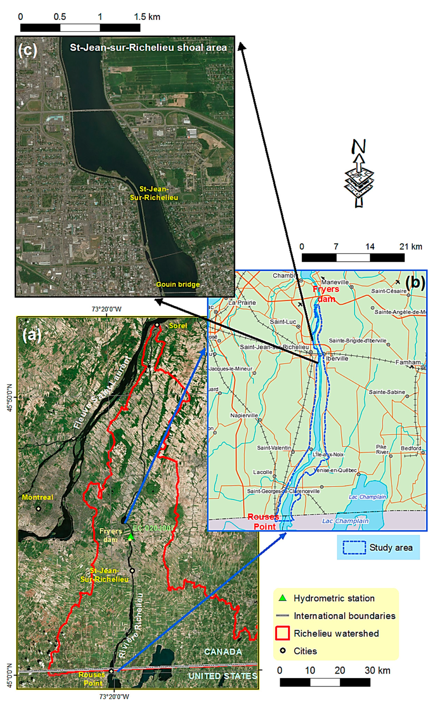
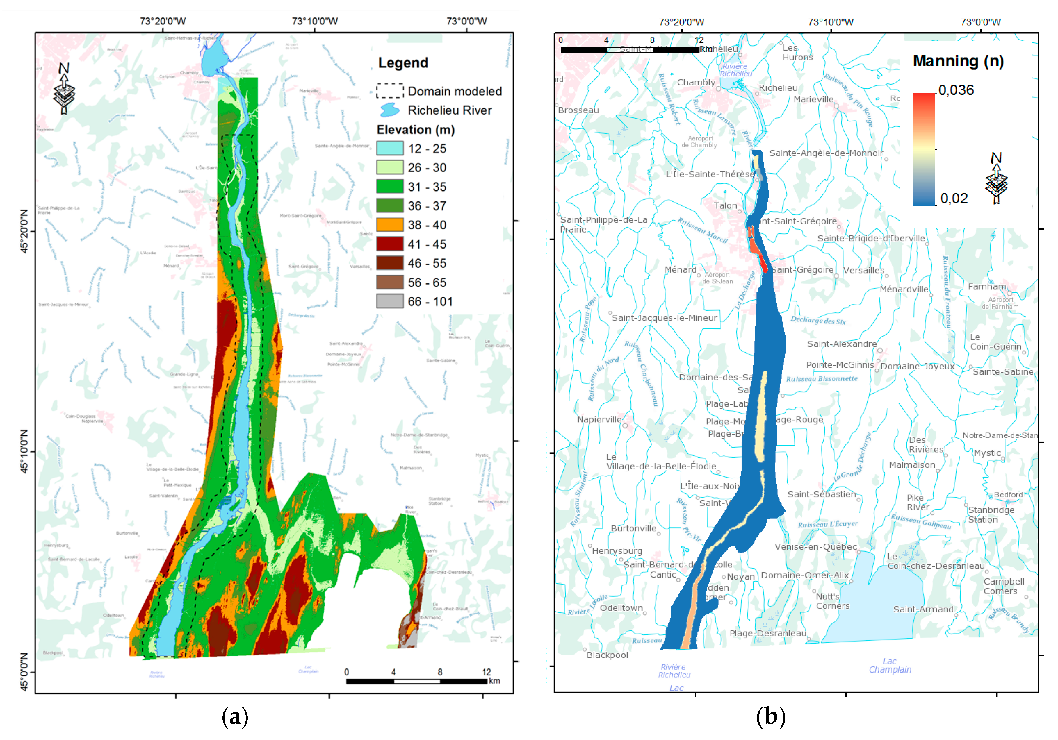
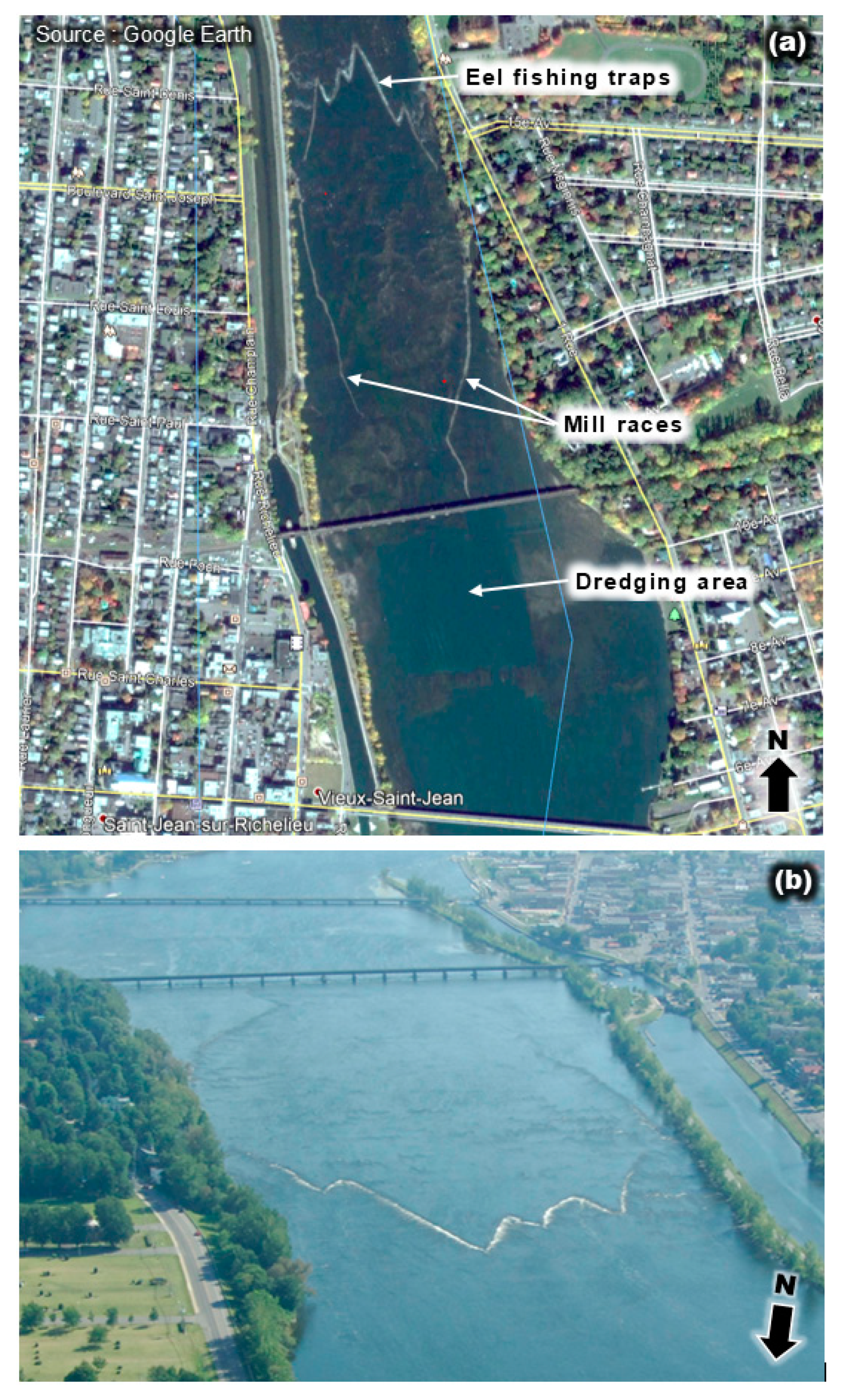
2. Hydraulic Model of Richelieu River

The Richelieu River watershed with a total area of 2506   km 2   is located about 20 km east of Montreal, Canada (Figure 1a). The Richelieu River takes its source from the Lake Champlain (at the U.S. border) and empties into the St. Lawrence River at the municipality of Sorel. The modelled 46 km long domain extends between Rouses point (NY) on the U.S–Canada border, and the Fryers Island Dam (QC), about 10 km downstream of the municipality of Saint-Jean-sur-Richelieu. The topography of the river is relatively flat with an average slope between these two points of about 0.3 m/km, including the relatively steep 24 m drop between the municipally of Saint-Jean-sur-Richelieu and the Fryer’s Dam through a series of rapids. The riverbed is mainly bedrock covered with shallow coarse sediments with a significant presence of shale clay and marine sediments dating from the post-glacial of Champlain Sea. The outflow rate from the Lake Champlain is controlled by a shoal located just downstream from Saint-Jean-sur-Richelieu (Figure 1c), forming a natural barrier to the flow. The study area has regularly experienced floods in the past. The most recent event occurred between 5 June and 4 August, 2011, registering a flow rate of up to 1539   m 3 / s , generating economic losses of more than 88 million dollars [58]. The May 2011 flood, as recorded at the Richelieu River at Rouses Point, was estimated to have a recurrence period equal to or greater than 1 in 500 years [59].
The starting point for the SA was the 2D finite element model H2D2 [60]. It was calibrated for the 2011 flood event under steady flow conditions and is assumed to best represent high flow rates [61]. The calibration accuracy itself is beyond the scope of this study. In the calibration process, the flow contributions from tributaries were ignored because of the significant storage capacity of the Champlain lake, which controls approximately 95% of the Richelieu River discharge into the Lawrence River [58]. The topography of the Richelieu River was determined with a DEM, generated from the available LiDAR data (Figure 2a). The DEM was with a 1 m grid with reported vertical accuracy of ±15 cm, whereas the vertical error specific to the airborne positioning system was estimated to be 3 cm. The river bathymetry was obtained from the Canadian Hydrographic Service (low river) and bathymetric transects were supplied by Parks Canada (mid river) [60].
For the present study, the topography and bathymetry data were assembled on an irregular hydrodynamic mesh with 97,261 nodes and 47,643 grid elements of 25 × 25 m. Significant man-made structures, including the Gouin Bridge at Saint-Jean-sur-Richelieu, were incorporated in the unstructured hydrodynamic mesh with the respective finite elements. Based on the available substrate sample observations, the calibrated Manning’s n coefficient for the Richelieu channel ranges from 0.02 to 0.036 (Figure 2b). The substrate upstream from the Gouin Bridge consists mainly of fine sand, silt, and some small boulders, while it is coarse and dominated by boulders and stones downstream from the Gouin Bridge. The flow data were available from the Fryers Rapids gauging station EC 02OJ007. The upstream boundary condition at Rouses Point was defined with a constant flow rate, while at the downstream end, near the station EC 02OJ007, a fixed water level was set, using the following stage-discharge relationship in Equation (1):
H   =   Q / 303.37 ( 1 / 1.727 )   +   25.52

3. The Sensitivity Analysis Method

The SA method proposed herein was conducted in the following successive steps: (i) Identification of the main input variables ( X 1   upstream flow rate, X 2   Manning’s n coefficient, and X 3 topography) for which the sensitivity of the depth of water as a model output is estimated; (ii) determination of the range of variation of the respective input variables; (iii) generation of samples of input values using the Gauss quadrature sampling; (iv) execution of the hydraulic model for each of these samples; and (v) estimation of the relative influence of each input variable in the model output by computing sensitivity indices.

3.1. Derivative-Based Sensitivity Indices

Central to the determination of the derivative-based sensitivity index is the perturbation of one input parameter at a time and computing, in parallel, the changes in the model output [62]. The output response to parameter perturbation may be quantified as a percentage of the selected output variable or as a relative change of the output versus input [63]. For determination of the sensitivity indices, a novel method of derivative-based sensitivity indices is proposed herein, based on the Gauss quadrature sampling.
First, the statistical properties of the input variables, such as the mean and standard deviation, are determined by respective probability distributions. In this study, the considered model output was the spatial distribution of the water depths produced by the 2D hydraulic model for each scenario. The SA is then performed varying the probability distribution of the model variables and analyzing the corresponding changes in the model output. For a model with i   input variables,   f ( X 1 , X 2 X i ) , the uncertain input normal random variable X i with a mean μ j , considered as a nominal parameter value, and a standard deviation, σ j , can be written as:
X i =   μ j + σ j ξ j ,
where   ξ j are independent identically distributed standard normal random variables corresponding to each input parameter. A nominal scenario f ( X i 0 ) is used to define the model output for the nominal value of X i . The focus is on the evaluation of the sensitivity index at the nominal value   μ i . The sensitivity can be defined as the partial derivative of f evaluated for the nominal scenario with respect to the input variable   X i .
S ( X i ) = [ f X i ] X i 0 ,
For easier understanding, the sensitivity can be considered as the rate of change of f due to change in X i . The relative sensitivity index S r can then be determined as a product of the absolute sensitivity and the ratio of the nominal input variable and the corresponding model output as follows:
S r ( X i ) = [ f X i ] X i 0   X i 0 f ( X i 0 ) ,
The relative sensitivity index (Sr) represents an estimate of the slope of the model response for the nominal value X   of the input variable in the parameter space [64]. Therefore, it was used to test the model sensitivity for each input variable. Higher value of the sensitivity indices indicates higher impact of an input parameter over the variability of the output [39]. An index value close to 0 indicates that the model output response to changes in the input is low or nil.
Given the complex nature of certain models, it can be difficult to approximate the partial derivatives with respect to the independent variables in Equation (4). To this end, a variety of methods exist to approximately compute the partial derivatives [65]. The finite difference method gradually varies each input variable by positive and negative increments around a nominal value, while keeping all the other input variables constant at their nominal value [66]. It is used as a sensitivity index in the context of local approaches [67]. Equation (4) can then be written in the following form:
S r ( X i ) =   [ Δ f ( X i ) Δ X i ] X j ,   j i 0   X i 0 f ( X i 0 ) ,
where Δ X i   is the range of variation around the nominal value, Δ f ( X i ) is the difference between the outputs for the two extremities of Δ X i , and X i 0   is the base scenario value. The input variables were each perturbed in turn by an amount of range of variation (interval) to compute the model outputs necessary to calculate the sensitivity index. While each input variable was perturbed, the other inputs were held at their mean values. Using an approximation of Equation (5), the computations of the sensitivity measures for i input variables require i + 1 model evaluations, using the difference method. This means that two runs of the model are needed for each of the three sensitivity coefficients and there is one sensitivity coefficient for each model input with respect to each model output. The computation of the derivative-based sensitivity indices is therefore computationally simple with relatively few model evaluations. The size of the applied perturbation assumed as an indication of the uncertainty needs to be sufficiently large to capture the whole set of variation of the model response and, at the same time, it has to be sufficiently small to avoid highly nonlinear or discontinuous changes in the output. The method is relatively simple in formulation when compared to other sensitivity analysis methods. In addition, it is relatively easy to execute, with the bulk of the effort required to utilize the method spent computing the sensitivity coefficients. The drawback of the method is that the derivative-based sensitivity indices provide information about local sensitivity only [39]. Certain shortcomings of the method also arise from the fact that it represents an approximate sensitivity analysis method.

3.2. Gaussian Quadrature Sampling

Global sensitivity analysis methods involve strategic sampling, e.g., such as the Sobol method with Latin hypercube sampling [68]. This strategy, however, needs many model runs in order to achieve the convergence. The sensitivity indices resulting from global sensitivity analysis are more accurate as they measure not only the individual effect of each input variable, but also the combined effect of the model inputs interacting with individual model inputs. In cases where it is not feasible to compute the sensitivity indices analytically with a large number of Monte Carlo simulations, an alternative sampling-based SA can provide useful information at acceptable computational costs. In this study, the method of Gauss quadrature was applied. The Gauss quadrature [69,70,71] is considered to be one of the best stratified sampling methods that use function values at sampling points with corresponding weights. An example of the application of the Gauss quadrature is the representation of random variables using Hermite polynomials of normally distributed random variables, known as Gauss–Hermite quadrature [72,73]. Three optimal sampling points based on Gauss quadrature were used. The choice of three points was made with a central point at x = μ x and two additional points of x + and x , symmetrically distributed at ± 3 σ   of the mean. The proposed method is therefore much simpler, as it significantly reduces the required number of model evaluations, constituting an efficient sampling strategy for considering scalar input variables (e.g., flow rate) and spatial variables (e.g., DEM and Manning’s n coefficient) at the same time.
In this study, the rate of change in each input variable was set to ± 3   of the corresponding standard deviation for the model input, reflecting their realistic possible ranges. Hence, three model runs are associated to each input variable, i.e., there are three perturbed DEMs, three flow rate values, and three sets of spatial distribution of the Manning’s n coefficient. The same interval was used in the calculations for the propagation of uncertainty. The applicability of this interval was found significant to lead a change in the calculation of a sensitivity index. In other words, the model outputs were calculated for three values of a given input variable: Nominal value, upper value ( + 3 uncertainty), and lower value ( 3 uncertainty). The sensitivity indices for each input variable of the 2D model were computed using Equation (5) independently.

3.3. Settings of Input Variables

3.3.1. Flow Rate

To consider the variation range of the flow rate, the reference flow for the hydraulic model was determined by performing frequency analysis of daily average flows measured at the Fryers Rapids station, available from 1970 to 2011. Frequency analysis was used to assess the specific flow rate uncertainty characteristics. To fully investigate the uncertainty in the potential flood events, four flow rates variables were imposed to constrain the model: 759, 824, 936, and 1113   m 3 / s . These values are related to return periods of 1.25, 1.4, 2, and 5 years, respectively. These scenarios are dynamic and defined as flood thresholds by Quebec’s Public Safety department. In addition, they were selected to study the effect of the shoal by increasing the flow rate from 759 to 1113   m 3 / s . The flow rate was assumed to be normally distributed, which is asymptotically true for most quantile estimators [74].
The respective mean discharge   μ Q , and the ± 3 σ flow rate values used as potential perturbed boundary condition realizations to compute the sensitivity indices are given in Table 1.

3.3.2. Manning’s n Coefficient

The Manning’s n coefficient in the 2D hydraulic model was inferred from substrate samples and land use maps. The Manning’s n coefficient varies spatially over the domain in the range between 0.02 and 0.036 for both the channel and the floodplain. These values are subject to uncertainty and therefore treated as random variables in the model. Changing the Manning’s n coefficient provides some control over the flow velocity. The 3 σ   rule [75] was applied, assuming statistically heterogeneous variation range with normal distribution [1,29,34]. The normal distribution has been used in similar studies [14] and, in the absence of information to contradict the normal assumption, it appears to be a reasonable approach. The calibrated Manning’s n values are assumed to be the mean values for the purposes of sensitivity analysis. The standard deviation of the probability density function (PDF) was calculated with the observed range [ M min , M max   ] of Manning’s n coefficient, using the following formula:
σ = ( M max M min ) / 6 ,
Equation (6) gives a standard deviation of the respective PDF for the domain of 0.0026. In this study, three Manning’s n coefficient maps were developed based on the Gauss quadrature to evaluate the sensitivity indices. It involves changing the Manning’s n coefficient along the river by the 3   σ error. An increase in the coefficient (upper scenario) yields a lower flow and a higher water level. Likewise, a decrease in the coefficient (lower scenario) includes shallow water depth, faster velocities, and supercritical flows.

3.3.3. Topography

The uncertainty related to terrain elevations in each DEM cell was generated by interpolating the standard deviation error assessed by kriging over the topographic measurements. The errors related to model topography were assumed with normal distribution and were introduced into the model evaluation using model simulations. To approximate the uncertainty in the topography, normal distribution was suggested [76,77]. The variance was then transformed into a standard deviation error using kriging, performed applying a locally adaptive variogram model with a sill of 0.8 and a nugget effect of 0.03 for the entire study area. In this way, a synthetic topographic surface was generated. To further assess the spatial sensitivity of the simulated water depths to the topography, the ± 3     krigged standard deviation of 21 cm was added and subtracted from the nominal topography model to obtain the upper and lower surfaces ( ± 3   σ ). Figure 3 gives the random field of the topography error together with the mean topography map and two realizations of the topography generated by perturbing the mean topography by the ± 3   random error.

4. Results and Discussion

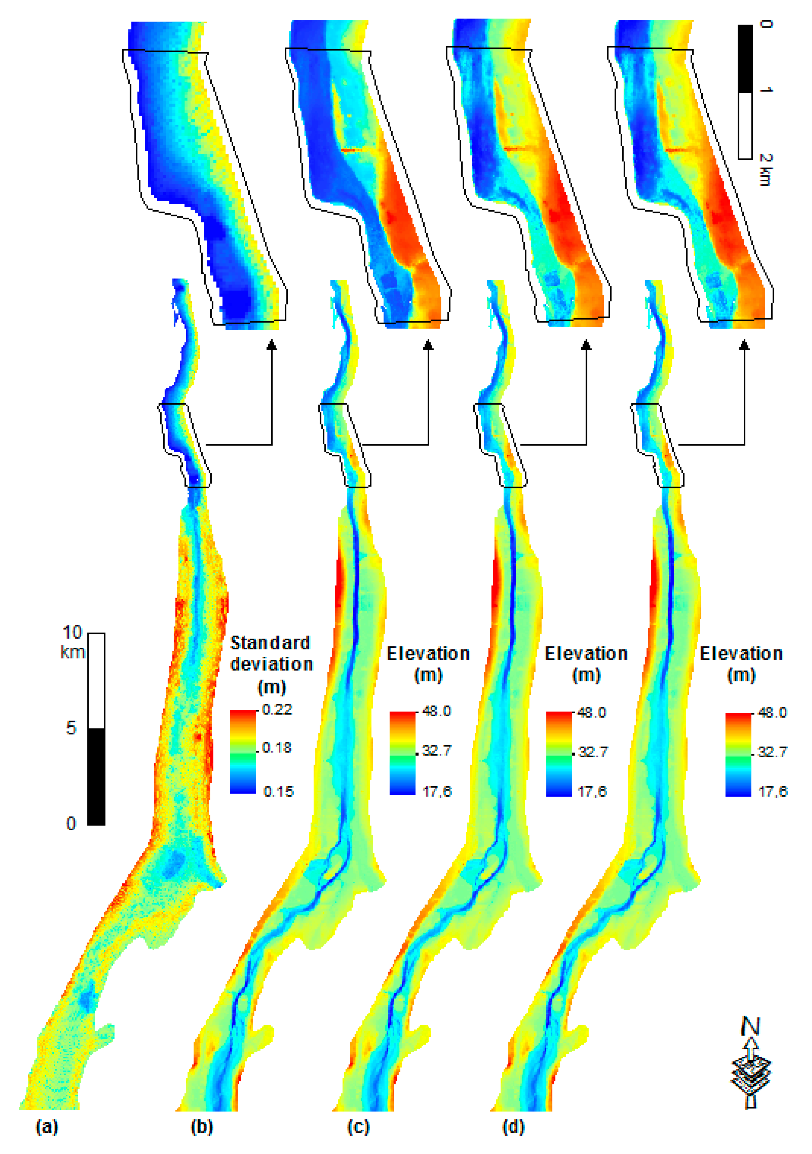
4.1. Water Depth Outputs

The sensitivity indices for each input variable were computed for the considered output model variable, the water depths in this case, predicted over the study domain. The water depth information under the surface was obtained by subtracting the local elevation of the ground (provided by the DEM) from the water surface elevation provided by the 2D hydraulic model. The simulated water depths for the nominal flow regimes of 759, 824, 936, and 1113 m 3 / s are shown in Figure 4. The respective overall mean water depths were computed as 4.38, 4.69, 4.83, and 4.68 m, respectively.
A visual comparison of Figure 4 brings out areas with high water depths located in the downstream section. The reach from Rouses Point to Saint-Jean-sur-Richelieu is characterized by shallower water depths, implying that this region can be considered an extension of Lake Champlain.

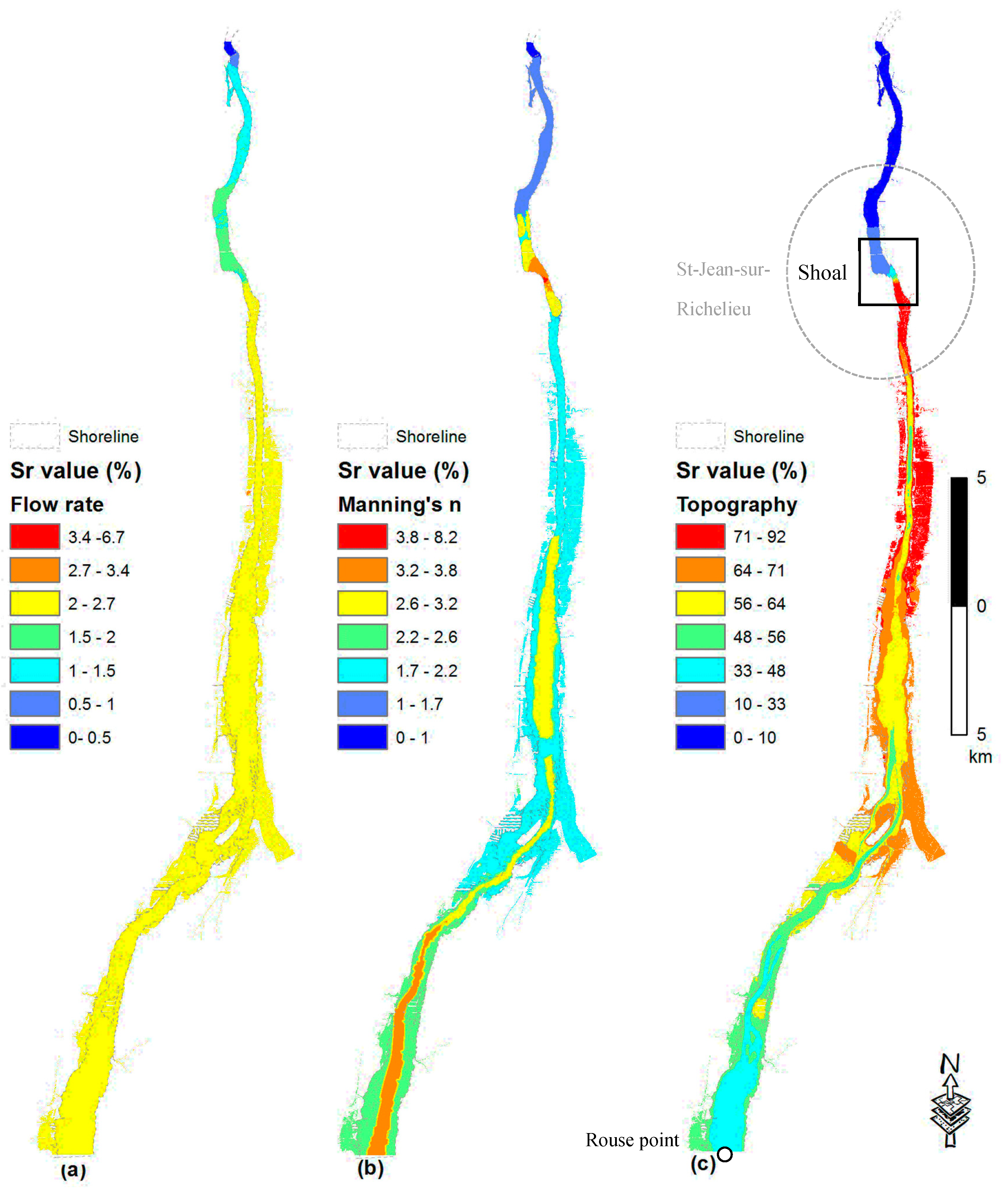
4.2. Results of Sensitivity Analysis

The spatial distribution of the relative sensitivity S r ( X i ) for each of the input variables, flow rate ( X 1 ) , Manning’s n coefficient   ( X 2 ) , and topography ( X 3 ) , was denoted respectively as   S r ( X 1 ) ,   S r ( X 2 ) ,   S r ( X 3 ) and obtained applying Equation (5). The computation of sensitivity index maps of water depths for the considered flow regimes of 759, 824, 936, and 1113 m 3 / s   is shown in Figure 5, Figure 6, Figure 7 and Figure 8. The sensitivity index reflects the degree of influence of the model inputs on the model outputs and does not indicate how much uncertainty the model input contributes. Positive coefficients mean that the computed value, water depth, changes in the same direction as the model input.
In general, the results show that the computed spatial distributions of the sensitivity indices for the input variables are different for different flow regimes (Figure 5, Figure 6, Figure 7 and Figure 8):
(i)
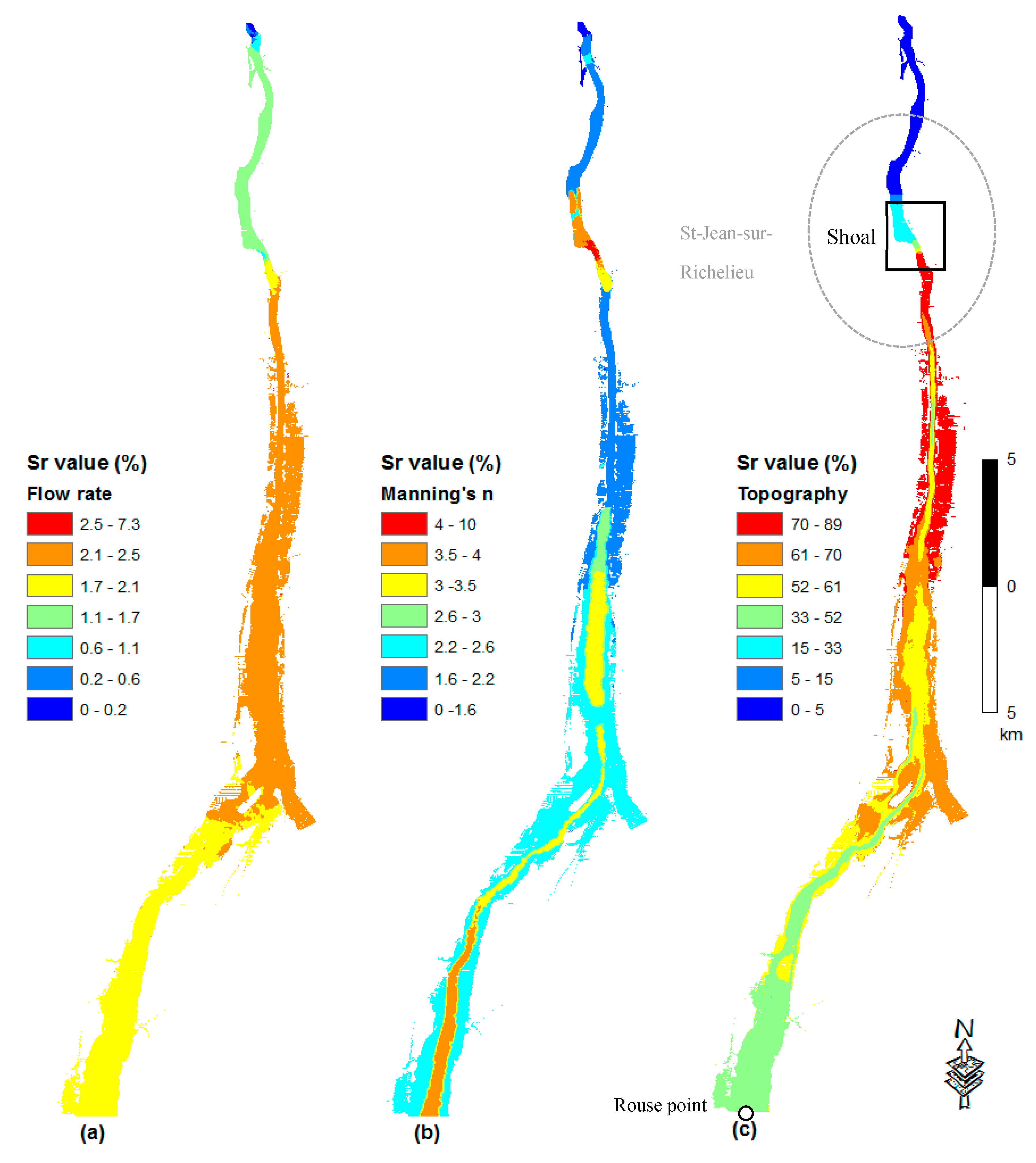
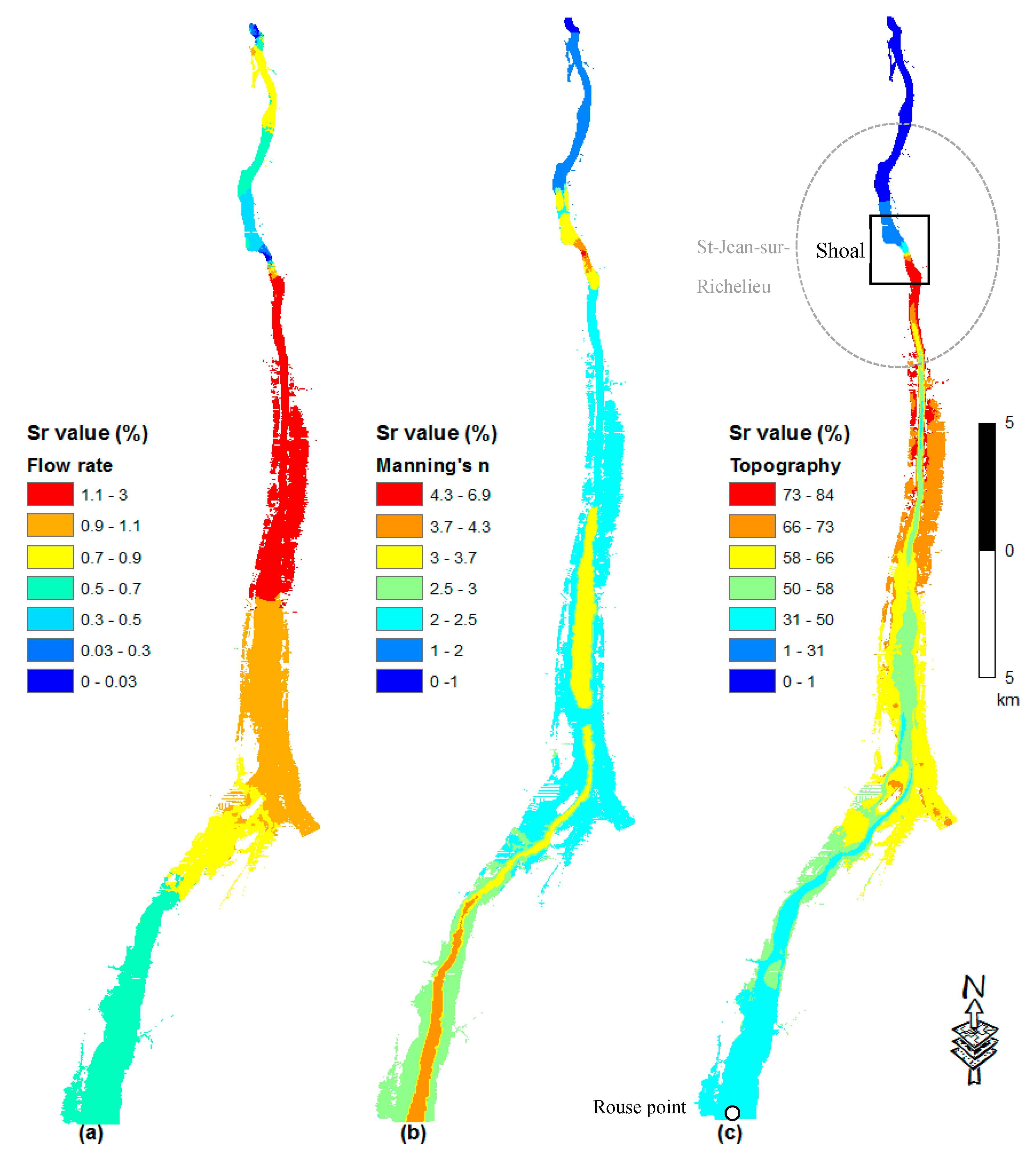
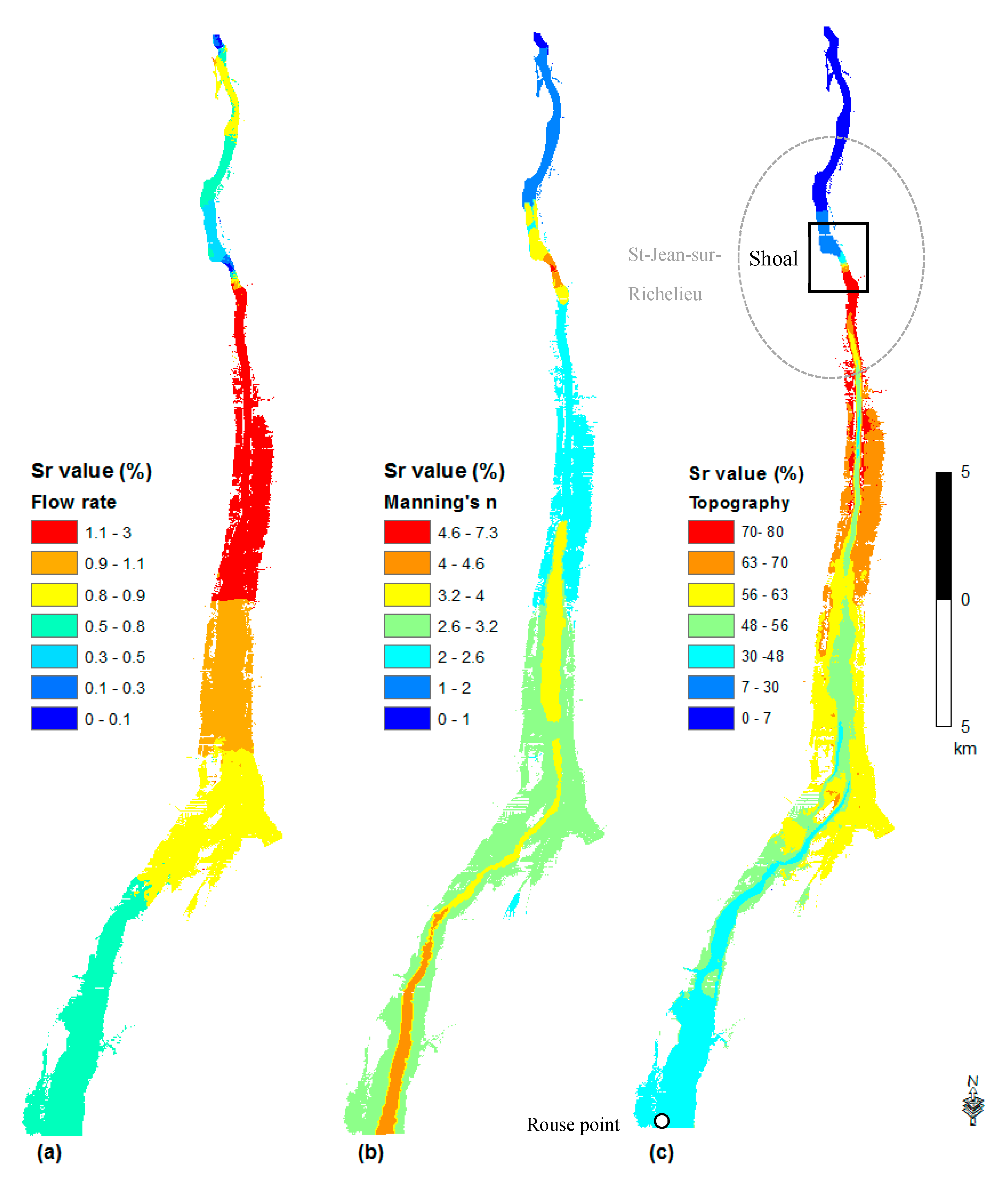
The sensitivity index for the topography values are the highest, indicating highest impacts on the computed water depths, particularly just upstream of the shoal. At the same time, the Manning’s n coefficient and the flow rate have comparatively lower Sr values. The sensitivity index for the computed water depths, with respect to the topography S r ( X 3 ) , is highest close to the Saint-Jean-sur-Richelieu shoal area, and decreases gradually further upstream (Figure 5c, Figure 6c, Figure 7c and Figure 8c). This observation suggests that upstream water depths are influenced by the shoal at Saint-Jean-sur-Richelieu, which exerts major control on the hydraulic system for all depth ranges and outflow rates from Lake Champlain;
(ii)
The sensitivity index for the flow rate,   S r ( X 1 ) , in each regime is lower in the upstream part and gradually increases in the downstream direction until the shoal, to drop again further downstream (Figure 5a, Figure 6a, Figure 7a and Figure 8a). Such spatial distribution of sensitivity indices for flow rates is most probably due to the influence of the upstream boundary at Rouses Point;
(iii)
On the other hand, the sensitivity index for Manning’s n coefficient, S r ( X 2 ) , is higher for areas where high values of the coefficient were measured, especially in a steep slope and where the riverbed is composed of a coarser substrate (Figure 5b, Figure 6b, Figure 7b and Figure 8b). Among these areas, the rapids of Saint-Jean located at shoal are the most sensitive to the Manning’s n coefficient. Thus, the impact of Manning’s n coefficient on water depth predictions is rather local. This can be explained by the fact that higher Manning’s n coefficients increase the frictional force of the water flow in the channel, reducing the flow velocity and consequently increasing the water level so that more water spreads outside of the bank. In the upstream direction, the sensitivity index to Manning’s n coefficient decreases to compensate the increased flow rate. At the upstream end of the studied reach, Manning’s coefficient contributes more to the uncertainty of the model output than the flow rate (Figure 5b, Figure 6b, Figure 7b and Figure 8b).
It can be observed in Figure 5, Figure 6, Figure 7 and Figure 8 that the effect of the shoal topography on the simulated water depths decreases for higher discharge rates. This can be explained by the fact that for river discharges higher than the bankfull discharge, the impact of modifications of river geometry on water depths mainly occurs in the main channel of the Richelieu River [78]. In addition, the Saint-Jean-sur-Richelieu shoal area contains some anthropogenic structures as steel traps for fishing nets and mill races (Figure 9). At low flow rates, these man-made structures fill with water without contributing to the flow because the velocities are very low, and probably act as a natural barrier at low flow rates. The preponderant effect of the shoal on both low and high flow regimes was the reason that the hydraulic model for the Richelieu River was calibrated solely for high water events of 6 May 2011, using a flow rate of 1539 m 3 / s . For this reason, and in order to build an accurate 2D hydraulic model, the topography of the model should be carefully considered, especially in the shoal proximity, by acquiring the best river bathymetry possible. The improved topography will help to improve model performance and therefore a good calibration for the entire range of the flow rate. If there are errors in the bathymetry, the Manning’s n values that are determined through calibration to water depths would compensate for these errors.
The quantified sensitivities reflect the degree of influence of the model inputs on the model outputs without indicating the contribution of the input uncertainty on the results. There are also limitations in extrapolating these findings to other hydrological settings. They are valid for a single model at a given location and flood event, and rely on the applied SA method. The obtained variability of the sensitivity of the water depth results is consistent with findings of Wilson and Atkinson [79], who showed that even a small degree of uncertainty in bed elevation can have a relatively large effect on water depth predictions. Horritt [28] came to a similar conclusion, pointing out the importance of the channel bathymetry in bank flow hydraulics. Despite this fact, one could intuitively expect that the computed sensitivities and ranking of input parameters should be different at different locations and different settings [17]. For example, for a smaller flood event with stages below bankfull conditions or where the bankfull level has been barely reached, uncertainties in the boundary conditions and Manning’s n parameters should be more important to consider, as they will be decisive to determine water depths and whether the bankfull discharge is attained or not. However, this may not be the case for large flood events. It would also be possible to apply a similar approach to assess the comparative influence of other discrete choices, such as the choice of hydraulic model (comparing 1D and 2D models), spatial resolution of DEM, etc. In any case, it is important for future studies to carefully consider the definition of the variability interval of input parameters to reduce or eliminate the influence on the sensitivity indices.

5. Conclusions

A sensitivity analysis (SA) was conducted for a 2D hydraulic model and individual impacts of three input variables: Topography, flow rate, and Manning’s n coefficient were quantified. Sensitivity coefficients were calculated for each input variable with respect to the simulated water depths. The method was tested and validated for a 2D hydraulic model of a 45 km long reach of the Richelieu River, Canada. This study provides an insight into models’ parameters and, in particular, their impacts on the simulated results.
The results indicate that the topography was the most critical input variable with the highest impact on the flood predictions. The effect of the topography on water depths was, however, attenuated for higher flow rates. On the other hand, Manning’s coefficient and the flow rate were comparatively less influential. In addition to the high quality LiDAR data, these results emphasize the need for accurate bathymetry and spatial distribution of the Manning’s coefficient in order to obtain better calibrated hydraulic models.
The standard SAs are based on hundreds or thousands of runs of the hydraulic model in order to test the numerous combinations of the system inputs. Applying traditional SA methods significantly increases the associated computational effort and often it is even impossible to run SA for practical cases where computer codes require several hours (or even several days) for a single simulation. Therefore, the scientific merits of the presented study are, first of all, in a considerably decreased computational effort, required to undertake SA of a 2D hydraulic model. Although the results are mathematically only approximate, this allows the user to test a number of perturbations to input variables, still obtaining results with satisfying accuracy. Therefore, instead of evaluating the sensitivity of one uncertain variable on the flood inundation, it is now possible to rapidly evaluate relative uncertainties among multiple variables and their propagation to the model outcome and, in this way, to provide improved understanding of the impacts of uncertain variables in flood inundation modelling. Subsequent work should focus on quantification of the sensitivity of model results to other input parameters, such as velocity, that differ for events of a different magnitude and at different locations. Additionally, it would be useful to explore the impact of the spatial resolution of DEM on the spatial variation in flood inundations. Overall, the study results contribute to informed decision-making, regarding the strategies for reducing model uncertainties.

Author Contributions

The authors designed and performed the research together. K.O. wrote the draft of the paper. K.C., M.N., Y.G., R.L., S.R., and J.P. made comments and corrections.

Funding

This research was funded by the Canadian Safety and Security Program led by Defence Research and Development Canada’s Centre for Security Science in partnership with Public Safety Canada (CSSP-2013-CP-1023).

Acknowledgments

This work was conducted by the Institut National de la Recherche Scientifique—Eau, Terre, Environnement in collaboration with Natural Resources Canada under the project entitled: Développement et application d’un outil de Gestion et Analyse du Risque d’Inondation sur le système transfrontalier du Lac Champlain—Rivière Richelieu (GARI). The authors gratefully acknowledge the contributions from Environment Canada and International Joint Commission.

Conflicts of Interest

The authors declare no conflict of interests.

References

  1. Cesare, M. First-order analysis of open-channel flow. J. Hydraul. Eng. 1991, 117, 242–247. [Google Scholar] [CrossRef]
  2. Neal, J.; Fewtrell, T.; Trigg, M. Parallelisation of storage cell flood models using OpenMP. Environ. Model. Softw. 2009, 24, 872–877. [Google Scholar] [CrossRef]
  3. Peña, F.; Nardi, F.J.H. Floodplain terrain analysis for coarse resolution 2D flood modeling. Dimensions 2018, 5, 52. [Google Scholar] [CrossRef]
  4. Sampson, C.C.; Smith, A.M.; Bates, P.D.; Neal, J.C.; Alfieri, L.; Freer, J. A high-resolution global flood hazard model. AGU 100 2015, 51, 7358–7381. [Google Scholar] [CrossRef] [PubMed]
  5. Sanders, B.F.; Schubert, J.E.; Detwiler, R.L. ParBreZo: A parallel, unstructured grid, godunov-type, shallow-water code for high-resolution flood inundation modeling at the regional scale. Adv. Water Resour. 2010, 33, 1456–1467. [Google Scholar] [CrossRef]
  6. Aronica, G.; Hankin, B.; Beven, K. Uncertainty and equifinality in calibrating distributed roughness coefficients in a flood propagation model with limited data. Adv. Water Resour. 1998, 22, 349–365. [Google Scholar] [CrossRef]
  7. Bates, P.D.; Horritt, M.; Hunter, N.; Mason, D.; Cobby, D. Numerical Modelling of Floodplain Flow; John Wiley and Sons Ltd.: Chichester, UK, 2005. [Google Scholar]
  8. Crosetto, M.; Tarantola, S.; Saltelli, A. Sensitivity and uncertainty analysis in spatial modelling based on GIS. Agr. Ecosyst. Environ. 2000, 81, 71–79. [Google Scholar] [CrossRef]
  9. Di Baldassarre, G.; Montanari, G.A.; Lins, H.; Koutsoyiannis, D.; Brandimarte, L.; Blöschl, G. Flood fatalities in Africa: From diagnosis to mitigation. Geophys. Res. Lett. 2010, 37, 1–5. [Google Scholar] [CrossRef]
  10. He, M.; Hogue, T.S.; Franz, K.J.; Margulis, S.A.; Vrugt, J.A. Characterizing parameter sensitivity and uncertainty for a snow model across hydroclimatic regimes. Adv. Water Resour. 2011, 34, 114–127. [Google Scholar] [CrossRef]
  11. Apel, H.; Merz, B.; Thieken, A.H. Quantification of uncertainties in flood risk assessments. JRBM 2008, 6, 149–162. [Google Scholar] [CrossRef] [Green Version]
  12. Apel, H.; Merz, B.; Thieken, A.H.; Blöschl, G. Flood risk assessment and associated uncertainty. Nat. Hazard. Earth Sys. 2004, 4, 295–308. [Google Scholar] [CrossRef] [Green Version]
  13. Alliau, D.; De Saint Seine, J.; Lang, M.; Sauquet, E.; Renard, B. Étude du risque d’inondation d’un site industriel par des crues extrêmes: De l’évaluation des valeurs extrêmes aux incertitudes hydrologiques et hydrauliques. HAL 2015, 2, 67–74. [Google Scholar] [CrossRef]
  14. Hall, J.; Tarantola, S.; Bates, P.; Horritt, M. Distributed sensitivity analysis of flood inundation model calibration. J. Hydraul. Eng. 2005, 131, 117–126. [Google Scholar] [CrossRef]
  15. Jung, Y.; Merwade, V. Estimation of uncertainty propagation in flood inundation mapping using a 1-D hydraulic model. Hydrol. Process. 2015, 29, 624–640. [Google Scholar] [CrossRef]
  16. Nguyen, T.-M.; Richet, Y.; Balayn, P.; Bardet, L. Propagation des incertitudes dans les modeles hydrauliques 1D. Houille Blanche. 2015, 5, 55–62. [Google Scholar] [CrossRef]
  17. Pappenberger, F.; Beven, K.J.; Ratto, M.; Matgen, P. Multi-method global sensitivity analysis of flood inundation models. Adv. Water Resour. 2008, 31, 1–14. [Google Scholar] [CrossRef]
  18. Abily, M.; Bertrand, N.; Delestre, O.; Gourbesville, P.; Duluc, C.-M. Spatial Global Sensitivity Analysis of High. Resolution classified topographic data use in 2D urban flood modelling. Environ. Model. Softw. 2016, 77, 183–195. [Google Scholar] [CrossRef]
  19. Savage, J.T.S.; Pianosi, F.; Bates, P.; Freer, J.; Wagener, T. Quantifying the importance of spatial resolution and other factors through global sensitivity analysis of a flood inundation model. AGU100 2016, 52, 9146–9163. [Google Scholar] [Green Version]
  20. Dimitriadis, P.; Tegos, A.; Oikonomou, A.; Pagana, V.; Koukouvinos, A.; Mamassis, N.; Koutsoyiannis, D.; Efstratiadis, A. Comparative evaluation of 1D and quasi-2D hydraulic models based on benchmark and real-world applications for uncertainty assessment in flood mapping. J. Hydrol. 2016, 534, 478–492. [Google Scholar] [CrossRef]
  21. Butler, M.P.; Reed, P.M.; Fisher-Vanden, K.; Keller, K.; Wagener, T. Identifying parametric controls and dependencies in integrated assessment models using global sensitivity analysis. Environ. Model. Softw. 2014, 59, 10–29. [Google Scholar] [CrossRef]
  22. Jakeman, A.J.; Letcher, R.A.; Norton, J.P. Ten iterative steps in development and evaluation of environmental models. Environ. Model. Softw. 2006, 21, 602–614. [Google Scholar] [CrossRef]
  23. Nguyen, T.; De Kok, J.; Titus, M. A new approach to testing an integrated water systems model using qualitative scenarios. Environ. Model. Softw. 2007, 22, 1557–1571. [Google Scholar] [CrossRef]
  24. Singh, R.; Wagener, T.; Crane, R.; Mann, M.; Ning, L. A vulnerability driven approach to identify adverse climate and land use change combinations for critical hydrologic indicator thresholds: Application to a watershed in Pennsylvania, USA. Water Resour. Res. 2014, 50, 3409–3427. [Google Scholar] [CrossRef] [Green Version]
  25. Pappenberger, F.; Matgen, P.; Beven, K.J.; Henry, J.-B.; Pfister, L.; Fraipont, P. Influence of uncertain boundary conditions and model structure on flood inundation predictions. Adv. Water Resour. 2006, 29, 1430–1449. [Google Scholar] [CrossRef]
  26. Apel, H.; Aronica, G.; Kreibich, H.; Thieken, A. Flood risk analyses—How detailed do we need to be? Nat. Hazards 2009, 49, 79–98. [Google Scholar] [CrossRef]
  27. Werner, M.; Blazkova, S.; Petr, J. Spatially distributed observations in constraining inundation modelling uncertainties. Hydrol. Process. 2005, 19, 3081–3096. [Google Scholar] [CrossRef]
  28. Horritt, M. Stochastic modelling of 1-D shallow water flows over uncertain topography. J. Comput. Phys. 2002, 180, 327–338. [Google Scholar] [CrossRef]
  29. Horritt, M. A linearized approach to flow resistance uncertainty in a 2-D finite volume model of flood flow. J. Hydrol. 2006, 316, 13–27. [Google Scholar] [CrossRef]
  30. Cobby, D.M.; Mason, D.C.; Horritt, M.S.; Bates, P.D. Two-dimensional hydraulic flood modelling using a finite-element mesh decomposed according to vegetation and topographic features derived from airborne scanning laser altimetry. Hydrol. Process. 2003, 17, 1979–2000. [Google Scholar] [CrossRef]
  31. Eilertsen, R.S.; Hansen, L. Morphology of river bed scours on a delta plain revealed by interferometric sonar. Geomorphology 2008, 94, 58–68. [Google Scholar] [CrossRef]
  32. Nicholas, A.; Mitchell, C. Numerical simulation of overbank processes in topographically complex floodplain environments. Hydrol. Process. 2003, 17, 727–746. [Google Scholar] [CrossRef]
  33. Woodhead, S.; Asselman, N.; Zech, Y.; Soares-Frazão, S.; Bates, P.; Kortenhaus, A. Evaluation of inundation models. FLOODsite Project Report T08-07-01. 2007. Available online: http://www.floodsite.net (accessed on 14 May 2019).
  34. Johnson, P.A. Uncertainty of hydraulic parameters. J. Hydraul. Eng. 1996, 122, 112–114. [Google Scholar] [CrossRef]
  35. Domeneghetti, A.; Castellarin, A.; Brath, A. Effects of rating-curve uncertainty on the calibration of numerical hydraulic models. In Proceedings of the First IAHR European Congress, Edinburgo, Scotland, 4 May 2010. [Google Scholar]
  36. Muleta, M.K.; Nicklow, J.W. Sensitivity and uncertainty analysis coupled with automatic calibration for a distributed watershed model. J. Hydrol. 2005, 306, 127–145. [Google Scholar] [CrossRef]
  37. Saltelli, A.; Tarantola, S.; Chan, K.S. A quantitative model-independent method for global sensitivity analysis of model output. Technometrics 1999, 41, 39–56. [Google Scholar] [CrossRef]
  38. Helton, J.C.; Davis, F.J. Latin hypercube sampling and the propagation of uncertainty in analyses of complex systems. Reliab. Eng. Syst. Saf. 2003, 81, 23–69. [Google Scholar] [CrossRef] [Green Version]
  39. Norton, J. An introduction to sensitivity assessment of simulation models. Environ. Model. Softw. 2015, 69, 166–174. [Google Scholar] [CrossRef]
  40. Devenish, B.; Francis, P.; Johnson, B.; Sparks, R.; Thomson, D. Sensitivity analysis of dispersion modeling of volcanic ash from Eyjafjallajökull in May 2010. J. Geophy. Res. Atmos. 2012, 117, 1–21. [Google Scholar] [CrossRef]
  41. Paton, F.; Maier, H.; Dandy, G. Relative magnitudes of sources of uncertainty in assessing climate change impacts on water supply security for the southern Adelaide water supply system. Water Resour. Res. 2013, 49, 1643–1667. [Google Scholar] [CrossRef] [Green Version]
  42. Tung, Y.K.; Yen., B.C. Hydrosystems Engineering Uncertainty Analysis; American Society of Civil Engineers: New York, NY, USA, 2005. [Google Scholar]
  43. Kucherenko, S.; Tarantola, S.; Annoni, P. Estimation of global sensitivity indices for models with dependent variables. Comput. Phys. Commun. 2012, 183, 937–946. [Google Scholar] [CrossRef]
  44. Oakley, J.E.; O’Hagan, A. Probabilistic sensitivity analysis of complex models: A Bayesian approach. J. R. Stat. Soc. Ser. B (Stat. Methodol.) 2004, 66, 751–769. [Google Scholar] [CrossRef]
  45. Helton, J.C.; Davis, J. Illustration of sampling-based methods for uncertainty and sensitivity analysis. Risk Anal. 2002, 22, 591–622. [Google Scholar] [CrossRef] [PubMed]
  46. Iman, R.L.; Helton, J.C. An investigation of uncertainty and sensitivity analysis techniques for computer models. Risk Anal. 1988, 8, 71–90. [Google Scholar] [CrossRef]
  47. Storlie, C.B.; Swiler, L.P.; Helton, J.C.; Sallaberry, C.J. Implementation and evaluation of nonparametric regression procedures for sensitivity analysis of computationally demanding models. Reliab. Eng. Syst. Saf. 2009, 94, 1735–1763. [Google Scholar] [CrossRef]
  48. Freer, J.; Beven, K.; Ambroise, B. Bayesian estimation of uncertainty in runoff prediction and the value of data: An application of the GLUE approach. Water Resour. Res. 1996, 32, 2161–2173. [Google Scholar] [CrossRef]
  49. Tang, T.; Reed, P.; Wagener, T.; Van Werkhoven, K. Comparing sensitivity analysis methods to advance lumped watershed model identification and evaluation. Hydrol. Earth Syst. Sc. Discussions 2006, 3, 3333–3395. [Google Scholar] [CrossRef]
  50. Borgonovo, E. A new uncertainty importance measure. Reliab. Eng. Syst. Saf. 2007, 92, 771–784. [Google Scholar] [CrossRef]
  51. Borgonovo, E.; Tarantola, S.; Plischke, E.; Morris, M. Transformations and invariance in the sensitivity analysis of computer experiments. J. Roy. Stat. Soc. Ser. B (Stat. Methodol.) 2014, 76, 925–947. [Google Scholar] [CrossRef]
  52. Pianosi, F.; Wagener, T. A simple and efficient method for global sensitivity analysis based on cumulative distribution functions. Environ. Model. Softw. 2015, 67, 1–11. [Google Scholar] [CrossRef] [Green Version]
  53. Pappenberger, F.; Beven, K.; Horritt, M.; Blazkova, S. Uncertainty in the calibration of effective roughness parameters in HEC-RAS using inundation and downstream level observations. J. Hydrol. 2005, 302, 46–69. [Google Scholar] [CrossRef]
  54. Kucherenko, S. Derivative based global sensitivity measures and their link with global sensitivity indices. Math. Comput. Simulat. 2009, 79, 3009–3017. [Google Scholar]
  55. Parajuli, P.B. SWAT Bacteria Sub-Model Evaluation And Application. Ph.D. Thesis, Kansas State University, Manhattan, KS, USA, January 2007. [Google Scholar]
  56. Chaubey, I.; Haan, C.; Salisbury, J.; Grunwald, S. Quantifying Model Output Uncertainty Due To Spatial Variability Of Rainfall. JAWRA 1999, 35, 1–11. [Google Scholar] [CrossRef]
  57. Khanal, S.; Parajuli, P.B. Sensitivity Analysis and Evaluation of Forest Biomass Production Potential Using SWAT Model. J. Sustain. Bioenerg. Systems 2014, 4, 136. [Google Scholar] [CrossRef]
  58. Riboust, P.; Brissette, F. Climate change impacts and uncertainties on spring flooding of Lake Champlain and the Richelieu River. JAWRA 2015, 51, 776–793. [Google Scholar] [CrossRef]
  59. Bjerklie, D.M.; Trombley, T.J.; Olson, S.A. Assessment of the spatial extent and height of flooding in Lake Champlain during May 2011, using satellite remote sensing and ground-based information. USGS 2014. [Google Scholar] [CrossRef] [Green Version]
  60. Secretan, Y. H2D2 Software. 2013. Available online: http://www.gre-ehn.ete.inrs.ca/H2D2/contenu_download (accessed on 14 May 2019).
  61. Boudreau, P.J.-F.; Cantin, A.; Bouchard, O.; Champoux, P.; Fiset, J.-M.; Fortin, N.; Guy Mori, J.T. Création d’un modèle hydraulique 2D de la rivière Richelieu entre Rouses Point et Sorel. Available online: https://legacyfiles.ijc.org/tinymce/uploaded/LCRRTWG/T%c3%a2che_2-3_Rivi%c3%a8re_Richelieu_2D_mod%c3%a9lisation_EC-SHN_FR.pdf(accessed on 14 October 2015).
  62. Youn, B.D.; Choi, K.K.; Du, L. Enriched Performance Measure Approach for Reliability-Based Design Optimization. AIAA J. 2005, 43, 874–884. [Google Scholar] [CrossRef]
  63. Larocque, M.; Banton, O. Determining parameter precision for modeling nitrate leaching: Inorganic fertilization in nordic climates. Soil Sci. Soc. Am. J. 1994, 58, 396–400. [Google Scholar] [CrossRef]
  64. Chokmani, K.; Viau, A.; Bourgeois, G. Analyse de l’incertitude de quatre modèles de phytoprotection relative à l’erreur des mesures des variables agrométéorologiques d’entrée. Agronomie. HAL 2001, 21, 147–167. [Google Scholar]
  65. Turanyi, T.; Rabitz, H. Local Methods. Sensitivity Analysis; Wiley: New York, NY, USA, 2000; pp. 81–99. [Google Scholar]
  66. Mitchell, A.R.; Griffiths, D.F. The Finite Difference Method In Partial Differential Equations; John Wiley: New York, NY, USA, 1980. [Google Scholar]
  67. Hill, M.; Tiedeman, C. Effective Calibration of Groundwater Models, with Analysis of Data, Sensitivities, Predictions, and Uncertainty; John Wiely: New York, NY, USA, 2007. [Google Scholar]
  68. Sobol, I.M. Global sensitivity indices for nonlinear mathematical models and their Monte Carlo estimates. Math. Comput.Simulat. 2001, 55, 271–280. [Google Scholar] [CrossRef]
  69. Babolian, E.; MasjedJamei, M.; Eslahchi, M. On numerical improvement of Gauss–Legendre quadrature rules. Appl. Math. Comput. 2005, 160, 779–789. [Google Scholar] [CrossRef]
  70. Dagde, K.K.; Akpa, J.G. Numerical Simulation of an Industrial Absorber for Dehydration of Natural Gas. Using Triethylene Glycol. J. Eng. 2014. [Google Scholar] [CrossRef]
  71. Tørvi, H.; Hertzberg, T. Estimation of uncertainty in dynamic simulation results. Comput. Chem. Eng. 1997, 21, S181–S185. [Google Scholar] [CrossRef]
  72. Abramowitz, M.; Stegun, I.A. Handbook of Mathematical Functions: With Formulas, Graphs, and Mathematical Tables; Courier Corporation: New York, NY, USA, 1964. [Google Scholar]
  73. Christian, J.T.; Baecher, G.B. Point-estimate method as numerical quadrature. J. Geotech. Geoenviron. 1999, 125, 779–786. [Google Scholar] [CrossRef]
  74. Stedinger, J.R. Confidence intervals for design events. J. Hydraul. Eng-Asce. 1983, 109, 13–27. [Google Scholar] [CrossRef]
  75. Pukelsheim, F. The three sigma rule: The American statistician. ASA 1994, 48, 88–91. [Google Scholar]
  76. Goncalves, J.; Oliveira, A. Accuracy analysis of DEMs derived from ASTER imagery. Intern. Arch. Photogramm. Remote Sens. 2004, 35, 168–172. [Google Scholar]
  77. Kornus, W.; Alamús, R.; Ruiz, A.; Talaya, J. Assessment of DEM accuracy derived from SPOT-5 high resolution stereoscopic imagery. Intern. Arch. Photogramm. Remote Sens. 2004, 35, 445–453. [Google Scholar]
  78. Di Baldassarre, G.; Claps, P. A hydraulic study on the applicability of flood rating curves. Hydrol. Res. 2011, 42, 10–19. [Google Scholar] [CrossRef]
  79. Wilson, M.; Atkinson, P. The use of elevation data in flood inundation modelling: A comparison of ERS interferometric SAR and combined contour and differential GPS data. Intern. J. River Basin Manag. 2005, 3, 3–20. [Google Scholar] [CrossRef]
Figure 1. The Richelieu River watershed (a), the study area (b), and the shoal area at Saint-Jean-Sur-Richelieu (c).
Geosciences 09 00220 g001
Figure 2. Digital Elevation Model (DEM) for the study area (a) and Manning’s n value for the studied river reach (b).
Geosciences 09 00220 g002
Figure 3. Three realizations of the random field of the topography error: Mean error (a), lower topography scenario (b), nominal (mean) topography model (c), and upper topography scenario (d).
Geosciences 09 00220 g003
Figure 4. Predicted water depth with the two-dimensional (2D) hydraulic model for flow cases of 759   m 3 / s   (a), 824   m 3 / s   (b), 936   m 3 / s   (c), and 1113   m 3 / s   (d) for nominal values of the topography and Manning’s n coefficient.
Geosciences 09 00220 g004
Figure 5. Sensitivity of the simulated flow depths for each of the three input variables, (a) flow rate   Sr ( X 1 ) , (b) Manning’s n coefficient   Sr ( X 2 ) , and (c) topography Sr ( X 3 ) , for nominal flow rate of 759   m 3 / s .
Geosciences 09 00220 g005
Figure 6. Sensitivity of the simulated flow depths to each of the three input variables, (a) flow rat e , (b) Manning’s coefficient Sr ( X 2 ) , and (c) topography Sr ( X 3 ) , for nominal flow rate of 824   m 3 / s .
Geosciences 09 00220 g006
Figure 7. Sensitivity of the simulated flow depths to each of the three input variables, (a) flow rate   Sr ( X 1 ) , (b) Manning’s n coefficient Sr ( X 2 ) , and (c) topography Sr ( X 3 ) , for nominal flow rate of 936   m 3 / s
Geosciences 09 00220 g007
Figure 8. Sensitivity of the simulated flow depths for each of the three input variables, (a) flow rate Sr ( X 1 ) , (b) Manning’s n coefficient Sr ( X 2 ) , and (c) topography Sr ( X 3 ) , for nominal flow rate of 1113   m 3 / s .
Geosciences 09 00220 g008
Figure 9. (a) Man-made structures in the Saint-Jean-sur-Richelieu bedrock shoal area. (b) Water surface disturbances caused by the remains of eel fishing structures.
Geosciences 09 00220 g009
Table 1. Quadrature Gaussian sampling: Flow rate values are in   m 3 / s .
μ σ x i 3 σ x i + 3 σ
75939.4690.75827.24
82436761.64886.35
93633.7877.62994.37
111339.41044.751181.24

