Abstract
Climate change is one of the prominent factors that causes an increased severity of extreme precipitation which, in turn, has a huge impact on drainage systems by means of flooding. Intensity–duration–frequency (IDF) curves play an essential role in designing robust drainage systems against extreme precipitation. It is important to incorporate the potential threat from climate change into the computation of IDF curves. Most existing works that have achieved this goal were based on Generalized Extreme Value (GEV) analysis combined with various circulation model simulations. Inspired by recent works that used machine learning algorithms for spatial downscaling, this paper proposes an alternative method to perform projections of precipitation intensity over short durations using machine learning. The method is based on temporal downscaling, a downscaling procedure performed over the time scale instead of the spatial scale. The method is trained and validated using data from around two thousand stations in the US. Future projection of IDF curves is calculated and discussed.
1. Introduction
The fourth National Climate Assessment (NCA) report [1] again alerted the community about the potential risks associated with climate change and the urgent need to take action. As part of the conclusion, the report projected that over the coming century, the increase in extreme climate events will continue, if not become more severe. A special report [2] by the Intergovernmental Panel on Climate Change (IPCC) in 2018 also concluded that human-caused global warming has reached up to 1.2 degrees Celsius compared to the global temperature in the pre-industry era. In addition, the global warming impact will reach up to 1.5 degrees Celsius in about 20 to 40 years, given the current pace of human activities. Such an increase in global warming has led to significant increases in the frequency of extreme weather events, particularly extreme precipitation [3]. Extreme precipitation can, in turn, cause various disasters including flooding, land sliding, and degradation of water quality.
One substantial type of damage caused by extreme precipitation is flash flooding, which has been studied in numerous previous works [4,5,6,7,8]. Flash flooding, usually referring to excessive overflowing of water within a six-hour duration, is one of the most damaging causes of the deterioration of water infrastructures and drainage systems. Most current risk management solutions to protect urban drainage systems against flash flooding are designed in accordance with the level of service (LoS) as well as the intensity of extreme precipitation, which is often described by the Intensity–Duration–Frequency curves (IDF curves) [9]. An IDF curve summarizes the averaged expected precipitation intensity of a precipitation event for a given duration and frequency. IDF curves are commonly used to quantify how extreme the precipitation is in a region. Both the American Society of Civil Engineers 24 (ASCE 24) standard [10] and the Federal Highway Administration report [11] provide the minimum design requirements for buildings and structures in flood hazard areas based on IDF curves. The most important range for the length of duration of an IDF curve spans from tens of minutes to hours, since these durations are highly relevant to the expected performance of many parts of drainage systems and their related structures.
Most drainage systems are designed based on a long service life cycle of up to tens of decades, but currently, not all design standards take the effect of climate change into consideration [12]. Many of the standards are made based on IDF curves computed from historical data, which essentially assumes that the historical statistics on extreme precipitation remain unchanged, even for future use. Such an assumption has been used by numerous prior works. For example, Huard et al. [13] used Bayesian estimation of IDF curves on historical data; Langousis and Veneziano [14] developed other methods for IDF curve computation targeted for settings when historical data are not abundant. However, such an assumption is becoming more and more unfounded as human interference increases. Therefore, incorporating climate change into the design of IDF curves is necessary.
Improving IDF curves to reflect the effect of climate change has attracted a lot of attention in recent years. The state-of-the-art method for future projection of IDF curves is based on the downscaled Global Climate Models (GCMs) or Regional Climate Models (RCMs). For example, DeGaetano and Castellano [15] used the Coupled Model Intercomparison Project 5 (CMIP5) daily GCM data for downscaled projection of IDF curves in the New York state. Hassanzadeh et al. [16] studied downscaling based on genetic programming and applied it to IDF curves. Herath et al. [17] studied how downscaling methods can be used to obtain IDF curves with a daily temporal resolution. Rodríguez et al. [18] used downscaling methods for IDF curves in the area of Barcelona. Mailhot et al. [19] used the Canadian Regional Climate Model (CRCM) to project and assess future IDF curves. To determine the precipitation intensity over short durations, more effort is required. For example, Wang et al. [20] used RCMs with high temporal resolution to compute IDF curves with short duration. De Paola et al. [21] used two disaggregation models to generate hourly data from daily precipitation data. Based on these disaggregation techniques, future IDF curves with short durations were projected. Haerter et al. [22] studied the the tail distribution of precipitation intensity over different durations. They concluded that for durations shorter than 30 min, the tail distribution follows an exponential scaling pattern more closely, while the tail follows a power law scaling for longer durations.
This study proposes an alternative method for determining the future extreme precipitation intensity for short durations. The goal is to design a method that can produce IDF curves for short durations (less than six hours) using only daily precipitation data. This is inspired by the observation that some commonly used downscaling methods only output daily precipitation simulations. For example, a very recent downscaling effort, called the NASA Earth Exchange program (OpenNEX 2018) [23], provides three sets of data: NASA Earth Exchange Downscaled Climate Projections (NEX-DCP30), NEX Global Daily Downscaled Projections (NEX-GDDP), and Localized Constructed Analogs (LOCA). NEX-DCP30 provides monthly summaries of the data; NEX-GDDP and LOCA provide only daily summaries.
This work achieves the above goal by temporal downscaling, also known as temporal disaggregation [21]. Inspired by recent works that use machine learning techniques for spatial downscaling [24,25,26], this work proposes a machine-learning based method that performs temporal downscaling from the daily precipitation intensity to the precipitation intensity for short durations. Because this method only needs daily downscaled GCM data, many downscaled GCMs with daily simulations but not sub-daily simulations can now be used to compute IDF curves. The method is cross-validated by around two thousand observational stations in the US and projections are provided.
This paper is organized in the following way: In Section 2, a detailed discussion of some related background knowledge is provided. Then, Section 3 introduces the details of the proposed method as well as how it is validated. The following Section 4 presents the analysis of the method applied to observation data in the US as well as the projected IDF curves. Finally, the conclusion and possible future directions are discussed.
2. Background
2.1. Intensity–Duration–Frequency Curves
As discussed in the introduction section, IDF curves are fundamental to the design of water infrastructures and drainage systems to make them resilient to extreme precipitation and flash floods. However, it is a non-trivial task to obtain IDF curves that reflect the intensity of extreme precipitation accurately. There are primarily two approaches to compute IDF curves, each with different advantages.
The first method used to produce IDF curves is to make assumptions on the precipitation distribution and then use mathematical tools to derive a formula for the IDF curves [27]. This method has become a popular way to compute IDF curves, and it is widely used in practice. Many prior works have explored what types of distribution can be used to get a higher accuracy when this method is applied to analyze IDF curves. One important family of distribution is the Generalized Extreme Value (GEV) distribution family. For example, Tfwala et al. [28] assumed that the precipitation distribution for each time interval follows the GEV distribution. Then, they computed the IDF curve based on the assumed distribution for each intensity and duration. Bougadis and Adamowski [29] studied scale invariances for disaggregating daily rainfall to hourly rainfall based on the scaling of GEV. Blanchet et al. [30] developed a GEV simple-scaling model to correct extremes of aggregated hourly rainfall. The use of GEV assumes that the precipitation levels over consecutive time intervals are independent of each other. This can be guaranteed by, for example, using a subsampling method [31,32].
The second method is based on empirical analysis. The empirical analysis of an IDF curve directly makes assumptions about the formulas of IDF curves, which are summarized from historical observations. These formulas usually come with two or more degrees of freedom. Then, empirical results are gathered from historical results to fit the above formulas and determine the parameters in the formulas. There are many IDF empirical formulas, and some of the popular ones are listed below:
In the above equations, I represents the intensity of the precipitation, t represents the duration, and p is the return period. Other parameters must be decided and can vary depending on time and location. Equation (1) was initially proposed by Sherman [33] when studying precipitation in the Boston area. Equation (2) was studied by Chow et al. [34]. Note that these two equations do not have a return period as the input and thus can be used for a specific return period only. If more than one of the IDF curves is needed, then multiple fitting using their respective historical data is required.
The most widely used formula was initially proposed by Bernard [35] and is shown in Equation (3). Different from Equations (1) and (2), it also incorporates the return period and thus, needs one fitting to model all return periods. This equation is based on the fact that the tail distribution of the intensity follows the power law. When it comes to short durations, Haerter et al. [22] studied when such an assumption is true. They concluded that the power law holds when the duration is longer than 30 min. This paper mainly focuses on durations longer than 30 min when Equation (3) is reliable. If using this equation for durations much shorter than 30 min, a higher error is more likely to appear. The empirical approach has attracted much attention in the computing of IDF curves. For example, Singh and Zhang [36] explored the use of Equation (3) for empirical analysis in the context of urban drainage design. Jain and Pandey [37] reviewed numerous empirical methods, including both Equations (1) and (3); they also studied a copula-based method for IDF curve formation. Dar et al. [38] studied the application of Equation (3) with fitted parameters to study various areas in India.
2.2. Supervised Machine Learning
Supervised machine learning is one kind of machine learning algorithm. Such algorithms can learn a relational property from one dataset and then apply the relation to other datasets to predict how the data should look given the predicted relation. These algorithms have been used in many related works on studying precipitation. For example, Foresti et al. [39] used neural networks to model extreme precipitation; and a survey by Vandal et al. [24] used machine learning for statistical downscaling.
A supervised machine learning algorithm usually uses labeled data as the input and trains a model from it. This model can be used to predict the label of some unlabeled data. There are four concepts associated with any supervised machine learning algorithm:
- Features. Feature (X) refers to the properties of the data that are known for the training dataset and projection datasets.
- Label. Label (Y) refers to the property that is only known for the training dataset and is unknown in the projection dataset. The goal is to predict the label for projection data using their features.
- Training phase. This is a procedure where a set of data is available, such that both features and labels are given for each data entry. The training phase takes these data entries as input and produces a compact description, namely the ML model, which describes the input–output relationship.
- Prediction phase. This is a procedure where a set of data, namely the testing data, is given but with features without labels only. The procedure also takes the model obtained above as input and outputs a label for each entry of the training data.
A machine learning model is said to be good if the predicted labels are consistent with their actual values. The task of a supervised machine learning algorithm is to determine the labels of all data in the testing set by using information from the training dataset. Depending on the nature of the problem and the structure of the data, some machine learning algorithms can be more useful than others. State-of-the-art supervised machine learning algorithms include the supported vector machine, gradient boosting tree, deep neural networks, etc.
2.3. Spatial Downscaling
Projecting future climate is a difficult task because it depends on the human activity level, which is highly unpredictable. Additionally, the global climate system is very complicated, and it is difficult to model all variables in the system. Therefore, future projection of climate requires a significant amount of effort, which has led to the formation of the Coupled Model Intercomparison Project (CMIP), where numerous GCMs have been proposed. These models usually make a set of global simulations that are openly available to download for each Representative Concentration Pathway (RCP), and these simulations are one of the most reliable sources for the future projection of climate. One major drawback of these GCM simulations is that they are usually available on a daily basis and at a coarse spatial resolution, which limits their usage to the study of local areas. Downscaling is a commonly used procedure to incorporate localized spatial influence to the GCM simulation to obtain future projections with high spatial resolution. One popular approach is dynamic downscaling, where a simulation of high resolution is performed on the regions of interest to extrapolate details from global GCMs [40,41,42]. It is able to incorporate physical principles into the analysis easily, but it is computationally intensive and sensitive to bias.
Statistical downscaling is another popular approach for downscaling, which views the downscaling process from a statistical perspective to find the relational properties between global climate and local climate. Most existing statistical downscaling methods adopt an ad hoc way to find the downscaling relationship. Existing statistical downscaling methods all follow a similar paradigm, as summarized below:
- Find a parameterized model to abstract the downscaling relationship between the global climate and local climate. The model is usually parameterized by a set of values.
- Use historical data to fit the model and find the parameters for the model. These parameters are assumed not to change over time. Perform bias correction to the results using methods like the Constructed Analogue method [43].
- Compute the local climate data using the model with fitted parameters and the future global climate.
This paradigm has been used by many popular downscaling works, including the Bias Corrected Constructed Analogue (BCCA) [43], the Multivariate Adaptive Constructed Analogs (MACA) [44], LOCA [45,46], and NEX-GDDP [47]. They are mainly different in the way of bias correction. This paper uses downscaled GCM simulation results from the NEX-GDDP downscaling project to improve the geographic resolution. Other downscaling methods and GCM simulations can be used by the proposed method in a similar way.
3. Methods
3.1. Overview
The main goal of this study was to compute precipitation intensity over a short duration using only daily downscaled GCM simulation data by means of temporal downscaling. As the complexity of temporal downscaling can be high and temporal data is not as abundant as spatial data, some extra procedures are required. First, instead of obtaining downscaled hourly precipitation data for the duration of study, the downscaling is designed such that it can directly output the intensity of the precipitation for different lengths of time. This simplification hugely eliminates unnecessary steps. To compute such a mapping from projected daily data to the intensity of short durations, machine learning algorithms are adopted that can perform non-linear learning efficiently. A summary of the comparison among machine learning, spatial downscaling, and the proposed temporal downscaling is provided in Table 1.

Table 1.
Comparison of machine learning, statistical downscaling, and the proposed temporal downscaling.
All three procedures follow a similar sequence of steps, as follows:
- Obtain some number of entries with both properties and targets. Taking these entries as the input, compute a description of the relationship between the entry properties and the targets.
- Make the assumption that the relationship between properties and targets holds for the projected entries.
- Use the above relationship as well as the properties for the projected entries, then compute the target value of the projected entries.
The method discussed in the following text also works for the three steps above but in the context of short-duration intensity projection.
3.2. Detailed Steps
In the following, all steps of the proposed method are discussed in detail. In Figure 1, an overview of the procedure is illustrated.
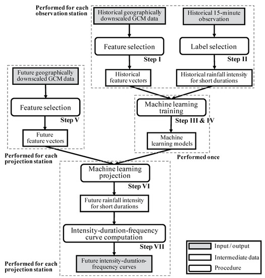
Figure 1.
Overview of the proposed method.
3.2.1. Step I: Historical Feature Selection
The first step is to select features for the use of machine learning training. Every station represents a different data entry, and a set of features is extracted. The source of the data used to extract the feature is downscaled GCM simulation data, which provide better geographic resolution. In principle, it is possible to use the downscaled GCM data directly as features, however in this case, the dimensions of the feature vector were too high for any machine learning algorithm to perform well. To reduce the dimensions of the features without affecting the learning accuracy, a set of features related to extreme precipitation and spatial information was selected. First, the following seven features were computed across all years for each station.
- 1.
- One-day and two-day precipitation intensities of the events with return periods of 2, 5, and 10 years.
- 2.
- Average daily precipitation.
Then, the average of the following 29 features across all years was computed for each station.
- 3.
- Number of rainy days.
- 4.
- Top 20 heaviest daily precipitation amounts in descending order.
- 5.
- Number of days with a daily precipitation of more than 5, 10, 15, 20, 30, 40, 50, and 60 mm.
Finally, the following 4 geographic features were extracted for each station.
- 6.
- Altitude of the location. This was obtained from the National Oceanic and Atmospheric Administration Climate Data Online (NOAA CDO).
- 7.
- The coordinates of the location, that is, latitude and longitude.
- 8.
- Climate division of the location. Since there are 344 climate divisions for the contiguous US [48], this feature had a value from 1 to 344. The use of climate division is to reinforce the geographic proximity between stations.
The above features are very popular in the analysis of extreme precipitation, including the US Climate Extremes Index (CEI) and the Expert Team on Climate Change Detection Monitoring and Indices (ETCCDMI) [49]. They result in a feature vector with 40 dimensions for each station. Note that due to the use of machine learning, it will be fairly easy to add more features in future research. This procedure needs to be performed for both historical observation stations as well as the stations used for future projections.
3.2.2. Step II: Label Selection
This paper uses the IDF formula based on Equation (3), where IDF curves for all durations can be expressed as a single equation: for a given duration t and return period p, the intensity is
For most regression models, the output label is a scalar number, but Equation (3) has 4 parameters to be determined. To be able to determine all parameters, the proposed method selects four different points on the IDF curve as the label (Y). In the proposed method, the four selected points are (1) return period 2 years, duration 30 min, (2) return period 2 years, duration 120 min, (3) return period 5 years, duration 30 min, and (4) return period 5 years, duration 120 min. The precipitation intensity for these four points needs to be extracted from the training data. It is done by calculating the precipitation intensity of the corresponding events from the historical data directly.
Note that choosing any 4 or more points can be used to fit Equation (3). However, if points are selected to be separated as much as possible then the resulting curves are more robust to potential noise in the data. The above four points are selected to be separated at the same time still located in short durations, which is the focus of this paper.
Another potential method for selecting ML labels is to select parameters in Equation (3) directly, namely the values of . In this potential method, all four parameters would be optimized by independent ML models. However, this can easily lead to local optimum parameter values that are far from being globally accurate. Therefore, this method is not selected, and the method based on the intensities of four selected points is used instead.
3.2.3. Step III: Model Selection
This step is used to select the ML model to learn the mapping from features to labels. Due to the nature of the projection, the machine learning algorithm should be able to work with continuous values, which means a regression algorithm is desired. As previously discussed in Section 2.2, the most powerful repression algorithms in machine learning are the Deep Neural Network (DNN) and the Gradient Boosting Tree (GBT). However, the DNN usually requires a very large amount of data because all layers of the neural network need to be fitted. Given these considerations, GBT is used as the main regression algorithm in this study.
3.2.4. Step IV: Future Feature Selection
This step is similar to Step I except that the feature selection is performed on future downscaled GCM data instead of the historical observation data.
3.2.5. Step V: Model Training
For each observation station, the features and label values are collected and used to train four models selected in previous steps. Each model can be used for projecting one data point on the future IDF curve.
3.2.6. Step VI: Machine-Learning Projection
To perform ML projection using GBT, three ML hyperparameters need to be decided: (1) The number of trees, which specifies the number of decision trees in the model; (2) the learning rate, which specifies the amount of contribution from each tree; and (3) the maximum depth, which specifies the maximum possible depth allowed in each decision tree. These hyperparameters can be determined by grid search with cross-validation, which is a common way for hyperparameter optimization and is supported in many ML software packages. After hyperparameters are decided, the model parameters can be decided as in the previous step. Note that due to the use of hyperparameter optimization, the validation is not completely independent to the data. There are numerous ways for validation to be conducted, which have been discussed in prior works in the context of hydrologic applications [50]. This work uses k-fold cross validation (see detailed discussion in Section 3.3). For each combination of model parameters, the validation is applied to find the best model parameters. After the model parameters have been selected and trained, projections are conducted on them. As a result, four data points on the projected IDF curves are obtained.
3.2.7. Step VII: IDF Curve Reconstruction
The last step is to use curve fitting to compute the IDF curves based on the four data points obtained above. The fitting algorithm used in this work is the expectation-maximization (EM) method with bounded conditions.
After step VI and the curve fitting as mentioned above, the parameters in Equation (3) are determined. Now, the precipitation intensity for other combinations of return periods and durations can be computed from the equation directly. This paper assumes that all combinations of return periods and durations follow this equation, which may not always be true. This assumption is validated in the next section before it is applied in the analysis.
3.3. Validation
3.3.1. k-Fold Cross Validation
A k-fold cross-validation method is applied, since it is widely used and has extensive software support. The detailed steps are as follows:
- Collect data from n stations. For a station, the data contains the downscaled GCM simulations of daily precipitation data and locally observed precipitation data with better resolution.
- Partition n stations of data into k disjoint and equal-sized sets, namely . Repeat the following step (step 3) k times.
- In the i-th repetition, use the i-th dataset as the test data (namely ), and the remaining data are used as training data (namely, ). Use the training data to train a machine learning model as described in the previous section and apply it to compute an IDF curve for stations in . Calculate the error based on the local precipitation testing data.
- Find the average of all errors in all k iterations above.
3.3.2. Validation of IDF Curves
Validation of the fitted IDF curves is performed by comparing the fitted precipitation intensity against the reference precipitation intensity provided from NOAA Atlas 14 [51], which provides the precipitation intensity for almost all states in the US.
The normalized root mean square error (NRMSE) metric and normalized mean absolute error (NMAE) are used, both of which measure the goodness-of-fit between the intensity from Atlas and the fitted ones. Similar metrics have been used to measure accuracy in prior works. For example, Chai et al. [52] compared RMSE and MAE when used for precipitation data and argued that both should be used when reporting errors. However, RMSE and MAE tend to be biased on data points with higher values. To avoid this bias, this paper uses these metrics with normalization where the relative differences are computed.
The definition of NRMSE is as follows: suppose is the intensity of precipitation with the time interval i and return period p in the observation; suppose is the same value computed from the analysis. For and ,
The definition of NMAE is similar and can be computed as
4. Analysis and Results
4.1. Data and Model Selection
Observation data were obtained from the data portal at the National Oceanic and Atmospheric Administration Climate Data Online (NOAA CDO) [53]. They provide historical year-round observations of data from 1970 to 2014 with a timescale of 15 min. Among all observation stations, only those with more than 25 years of observation were selected. The spatial distribution of all stations selected is shown in Figure 2. In total, 1936 stations were selected.
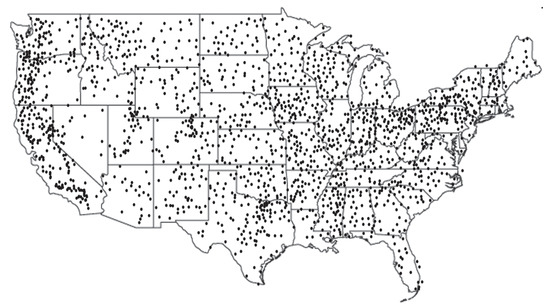
Figure 2.
Geographic distribution of all observation stations used to train the gradient boosting tree model. All data were obtained from the National Oceanic and Atmospheric Administration Climate Data Online (NOAA CDO) [53].
Reference precipitation intensity data used for validation were obtained from NOAA Atlas 14 project [51], where precipitation intensity data were available from all states except Washington, Oregon, Montana, Wyoming, and Idaho. These reference precipitation intensities were estimated by NOAA and were consistent with the actual precipitation intensity.
The downscaled GCM simulation data were based on Community Climate System Model 4 (CCSM4) with the NEX-GDDP downscaling method. The RCP 8.5 trajectory was extracted. The timescale of data was on a daily basis. The historical data were collected from 1970 to 2014, and from 2040 to 2099 for the future. The CCSM4 was developed by the National Center for Atmospheric Research (NCAR) in the USA. It consists of four different models, each simulating one component on the Earth’s atmosphere, ocean, land surface, and sea-ice—it also includes one central coupler component. Note that the downscaled GCM simulation results were used instead of the GCM results so that the obtained results had a better spatial resolution. All downscaling data can be obtained from NASA website [54]. Since this study mainly focused on the methodology, only one downscaled GCM result was used. Note that model-to-model variation can be high and can potentially influence the projection results.
The GBT models were trained based on data from 1936 stations. Eight representative stations were selected to show the projection results. They were selected to be spatially distributed across the US and have different IDF curve shapes. Details of the stations are summarized in Table 2.
Table 2.
Information about the eight representative stations.
4.2. Validation and Historical IDF Curves
Figure 3 shows the historical IDF curves for all eight representative stations. There are three sets of data shown in each figure:
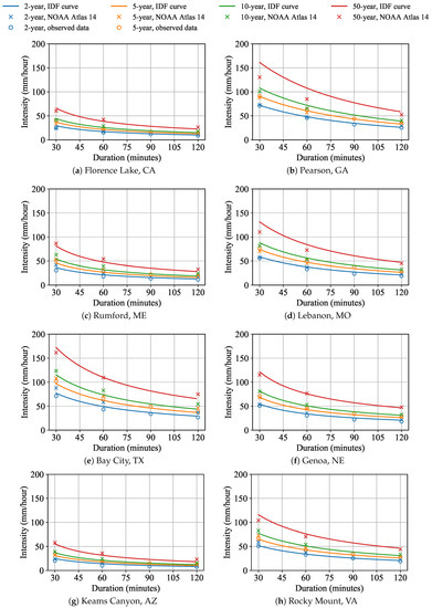
Figure 3.
Historical Intensity–Duration–Frequency (IDF) curves. The data points in “∘” are intensities computed using the observation data; data points in “×” are intensities extracted from NOAA Atlas 14. All solid lines were fitted using the observation intensity (in ∘) and plotted for high return periods.
- The ∘-shape data points represent precipitation intensity extracted from the historical data from NOAA CDO, with intensities of 30, 60, 90, and 120 min and return periods of 2 and 5 years.
- The solid lines are IDF curves fitted based on the above observed data using Equation (3). This equation was used for all return periods, and four IDF curves were plotted for return periods of 2, 5, 10, and 50 years.
- The ×-shape data points represent the precipitation intensity obtained from NOAA Atlas 14.
Since short-duration intensity is the focus of this study, duration was plotted from 30 min up to 120 min. The figure indicates that the shape of the IDF curves greatly depends on the location of the observation. Nevertheless, it is shown that the IDF curve for all figures fits well with the observed data, and the obtained IDF curves are consistent with the Atlas 14 precipitation intensity.
Each individual figure represents the historical precipitation intensity level in each region. The observation stations at Pearson, GA and Bay City, TX have the most extreme short-duration precipitation intensity, and with a 50-year return period, their 30-min intensity could be as high as 150 mm/h. Keams Canyon, AZ has a much lower level of precipitation intensity. Their 50-year return period 30-min intensity is about 50 mm/h.
To further quantitatively validate this approach, a comparison between the fitted IDF curve and the IDF data from NOAA Atlas 14 was performed. A relative difference ratio was computed as follows, where positive values represent overestimates and negative values represent underestimates.
Table 3 summarizes the computed ratios for all eight stations picked in this study. It can be observed from the table that most fitted intensity values are within of the Atlas 14 intensity values. Even for cases where a higher difference is observed, they are still within of the difference. It is also observed that the difference ratios for 120-min duration is higher than shorter durations in general. Because the intensities for 120-min are much smaller than shorter durations, the resulting difference ratios becomes larger given the same error in intensity. TX and ME have the largest error where many intensities are below the Atlas 14 intensities, resulting in negative difference ratios. For these locations, the observed intensities are also much less than the Atlas 14 intensities. This is believed to be the reason for a larger error for these locations.
Table 3.
Relative difference between fitted IDF intensity and NOAA Atlas 14 intensity.
Table 4 shows the goodness-of-fit between the IDF curve fitted from the observations and the intensity data from NOAA Atlas 14. As discussed in Section 3.3, NRMSE and NMAE were used. Smaller values of NRMSE and NMAE means higher accuracy. The table shows that the fitting errors are relatively small compared to the actual values of intensity. In Table A1 from the Appendix A, 44 stations from different states in the US are examined in a similar way with NRMSE and NMAE presented. NOAA Atlas 14 data from 5 states are not available and thus not included. Alaska is also not included due to lack of data. This table shows that even across a wide selection of areas, the error is relatively small with an average NRMSE and NMAE of about 0.1.
Table 4.
NRMSE and NMAE between fitted IDF intensity and the NOAA Atlas 14 intensity.
4.3. Projection Results
Future precipitation intensity was projected following the steps described in the previous section. The projected results are shown in Figure 4 for years 2040 to 2069; and in Figure 5 for years 2070 to 2099. The historical IDF curves are also shown with dotted lines for comparison. These figures show that the precipitation intensities are projected to increase in all locations, although the amount of increase is different. In more detail, Bay City, TX, and Pearson, GA are projected to suffer from greater increases in precipitation intensity. The intensity will increase by around 50 mm/h. The increases in Florence Lake, CA, and Keams Canyon, AZ are projected to be the smallest. More discussion on the relation between the intensity and the return period is included in the Appendix A.
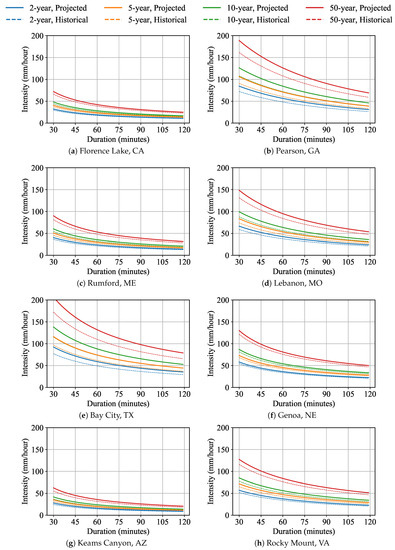
Figure 4.
Projected IDF curves from 2040 to 2069. Dotted lines are for historical IDF curves; solid lines are for projected IDF curves.
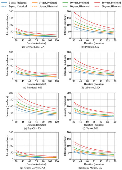
Figure 5.
Projected IDF curves from 2070 to 2099. Dotted lines are for historical IDF curves; solid lines are for projected IDF curves.
The increase ratio is further calculated based on the projection, which demonstrates the relative amount of increase across short durations. These ratios are shown in Table 5. From the table, it is observed that the ratio of increase is higher for locations with historically higher precipitation intensity (e.g., GA, TX, MO). It means that locations that suffers the most from the damage of extreme precipitation will witness even more extreme precipitation in the future, possibly because locations with higher intensities will be more vulnerable to climate change. The ratios are computed following the equation, as the average of all ratios at different locations on the IDF curves.
where and .
Table 5.
Ratio of increase for the projected IDF curves for the future based on downscaled GDDP GCM results using the CCSM4 downscaling method.
5. Conclusions
The expected precipitation intensity of short durations significantly affects the design of drainage systems. This work proposed an alternative method to improve the projection of IDF curves for short durations. The method is based on a temporal downscaling approach, which produces information for short durations based on the information from long durations. In more detail, a machine-learning based approach is used, where daily precipitation downscaled GCM data are used as feature values, and the precipitation intensity is used as the label values. By obtaining multiple intensity points, future IDF curves are projected with different duration and return period. One caveat of this method is the use of IDF equation to derive precipitation intensity, where it is assumed that the precipitation intensity of different return periods and durations follow some mathematical equation. This should always be validated first before used.
By using this method, downscaled GCM simulation data obtained from NASA NEX-GDDP project were used for future IDF curve projection. The historical precipitation intensity was obtained from NOAA CDO 15-min precipitation observed data. The data and IDF formula were further validated based on eight stations across the US. By comparing the fitted precipitation intensity against the Atlas 14 intensity, high accuracy was found. The projection results show that an increase in precipitation intensity of 10% to 20% may be observed in the next few decades.
Author Contributions
Conceptualization, H.H., B.M.A.; methodology, H.H., B.M.A.; validation, H.H.; data curation, H.H.; writing–original draft preparation, H.H.; writing–review and editing, B.M.A.; supervision, B.M.A.
Funding
This research received no external funding
Conflicts of Interest
The authors declare no conflict of interest.
Appendix A. Frequency Analysis on Precipitation Intensity
Figure A1 and Figure A2 show the same IDF-curves data but with x-axis as return period and different curves for different durations. It can be observed that for the each duration, the intensity increases as the return period increases.
Table A1.
NRMSE and NMAE between fitted IDF intensity and the NOAA Atlas 14 intensity. For 44 stations from different states in United States. Data from states AK, WA, OR, ID, MT, WY are not included due to lack of observation data or NOAA Atlas 14 data.
Table A1.
NRMSE and NMAE between fitted IDF intensity and the NOAA Atlas 14 intensity. For 44 stations from different states in United States. Data from states AK, WA, OR, ID, MT, WY are not included due to lack of observation data or NOAA Atlas 14 data.
| Station | Location | State | NRMSE | NMAE |
|---|---|---|---|---|
| 010140 | ALBERTA | AL | 0.109 | 0.077 |
| 034839 | MILLWOOD DAM | AR | 0.122 | 0.11 |
| 026119 | ORACLE 2 SE | AZ | 0.057 | 0.051 |
| 048025 | SAWYERS BAR RANGER STATION | CA | 0.145 | 0.117 |
| 052790 | EVERGREEN | CO | 0.111 | 0.104 |
| 066942 | ROCKVILLE | CT | 0.09 | 0.077 |
| 076410 | NEWARK UNIVERSITY FARM | DE | 0.142 | 0.12 |
| 083538 | GRACEVILLE 1 SW | FL | 0.067 | 0.062 |
| 093312 | FARGO | GA | 0.133 | 0.117 |
| 510055 | AHUIMANU LOOP | HI | 0.061 | 0.053 |
| 130608 | BELLEVUE L AND D 12 | IA | 0.087 | 0.075 |
| 114355 | ILLINOIS CITY DAM 16 | IL | 0.064 | 0.06 |
| 120830 | BLUFFTON 6 N | IN | 0.149 | 0.128 |
| 146024 | ONAGA 12 SSW | KS | 0.049 | 0.04 |
| 153929 | HODGENVILLE LINCOLN | KY | 0.169 | 0.12 |
| 161411 | CALHOUN RES STATION | LA | 0.144 | 0.134 |
| 190998 | BUFFUMVILLE LAKE | MA | 0.182 | 0.174 |
| 180700 | BELTSVILLE | MD | 0.11 | 0.078 |
| 170273 | AUGUSTA | ME | 0.048 | 0.039 |
| 200662 | BELLAIRE | MI | 0.06 | 0.054 |
| 218323 | TRACY | MN | 0.111 | 0.107 |
| 230204 | APPLETON CITY | MO | 0.076 | 0.065 |
| 227276 | RALEIGH 6 N | MS | 0.052 | 0.045 |
| 311241 | BURLINGTON | NC | 0.126 | 0.118 |
| 325993 | MINOT EXPERIMENT STATION | ND | 0.048 | 0.044 |
| 250075 | ALBION 7 W | NE | 0.107 | 0.089 |
| 273182 | FRANKLIN FALLS DAM | NH | 0.085 | 0.075 |
| 281351 | CAPE MAY 2 NW | NJ | 0.155 | 0.141 |
| 292700 | EAGLE NEST | NM | 0.215 | 0.207 |
| 264698 | LOVELOCK | NV | 0.2 | 0.193 |
| 309442 | WHITNEY POINT DAM | NY | 0.058 | 0.049 |
| 332272 | DOVER DAM | OH | 0.103 | 0.097 |
| 340179 | ALTUS IRIG RES STATION | OK | 0.07 | 0.062 |
| 369367 | WAYNESBURG 1 E | PA | 0.136 | 0.126 |
| 375215 | NEWPORT ROSE | RI | 0.209 | 0.208 |
| 383468 | GEORGETOWN 2 E | SC | 0.158 | 0.146 |
| 391452 | CARPENTER 4 NNE | SD | 0.066 | 0.06 |
| 406170 | MONTEREY | TN | 0.157 | 0.129 |
| 414679 | JUSTIN | TX | 0.105 | 0.077 |
| 420086 | ALTON | UT | 0.14 | 0.123 |
| 446475 | PAINTER 2 W | VA | 0.108 | 0.1 |
| 433914 | HIGHGATE FALLS | VT | 0.101 | 0.09 |
| 473038 | GENOA DAM 8 | WI | 0.049 | 0.044 |
| 463238 | FREEMANSBURG 5 NE | WV | 0.096 | 0.074 |
| Average | 0.110 | 0.097 |

Figure A1.
Projected intensity curves from 2040 to 2069. Dotted lines are for historical IDF curves; solid lines are for projected IDF curves.
Figure A1.
Projected intensity curves from 2040 to 2069. Dotted lines are for historical IDF curves; solid lines are for projected IDF curves.


Figure A2.
Projected intensity curves from 2070 to 2099. Dotted lines are for historical IDF curves; solid lines are for projected IDF curves.
Figure A2.
Projected intensity curves from 2070 to 2099. Dotted lines are for historical IDF curves; solid lines are for projected IDF curves.

References
- U.S. Global Change Research Program (USGCRP). Impacts, Risks, and Adaptation in the United States: Fourth National Climate Assessment, Volume II; USGCRP: Washington, DC, USA, 2018. [CrossRef]
- Intergovernmental Panel on Climate Change (IPCC). Summary for Policymakers. In Global warming of 1.5 °C. An IPCC Special Report on the Impacts of Global Warming of 1.5 °C above Pre-Industrial Levels and Related Global Greenhouse Gas Emission Pathways, in the Context of Strengthening the Global Response to the Threat of Climate Change, Sustainable Development, and Efforts to Eradicate Poverty; IPCC: Geneva, Switzerland, 2018. [Google Scholar]
- Ali, H.; Mishra, V. Increase in Subdaily Precipitation Extremes in India Under 1.5 and 2.0° Warming Worlds. Geophys. Res. Lett. 2018, 45, 6972–6982. [Google Scholar] [CrossRef]
- Newby, M.; Franks, S.W.; White, C.J. Estimating urban flood risk-uncertainty in design criteria. Proc. Int. Assoc. Hydrol. Sci. 2015, 370, 3–7. [Google Scholar] [CrossRef][Green Version]
- Madsen, H.; Lawrence, D.; Lang, M.; Martinkova, M.; Kjeldsen, T. Review of trend analysis and climate change projections of extreme precipitation and floods in Europe. J. Hydrol. 2014, 519, 3634–3650. [Google Scholar] [CrossRef]
- Krishnamurthy, L.; Vecchi, G.A.; Yang, X.; van der Wiel, K.; Balaji, V.; Kapnick, S.B.; Jia, L.; Zeng, F.; Paffendorf, K.; Underwood, S. Causes and probability of occurrence of extreme precipitation events like Chennai 2015. J. Clim. 2018. [Google Scholar] [CrossRef]
- Nogal, M.; O’Connor, A.; Martinez-Pastor, B.; Caulfield, B. Novel probabilistic resilience assessment framework of transportation networks against extreme weather events. ASCE-ASME J. Risk Uncertain. Eng. Syst. Part A Civ. Eng. 2017, 3, 04017004. [Google Scholar] [CrossRef]
- Tabari, H.; Willems, P. Anomalous Extreme Rainfall Variability Over Europe—Interaction between Climate Variability and Climate Change. In New Trends in Urban Drainage Modelling; Mannina, G., Ed.; Springer International Publishing: Cham, Switzerland, 2019; pp. 375–379. [Google Scholar]
- Mailhot, A.; Duchesne, S. Design criteria of urban drainage infrastructures under climate change. J. Water Resour. Plan. Manag. 2009, 136, 201–208. [Google Scholar] [CrossRef]
- Committee, A.S. Flood Resistant Design and Construction; Technical Report; American Society of Civil Engineers: Reston, VA, USA, 2005. [Google Scholar]
- Kilgore, R.T.; Herrmann, G.R.; Thomas, W.O., Jr.; Thompson, D.B. Highways in the River Environment- Floodplains, Extreme Events, Risk, and Resilience; Technical Report; Federal Highway Administration: Washington, DC, USA, 2016. [Google Scholar]
- Saini, A.; Tien, I. Impacts of climate change on the assessment of long-term structural reliability. ASCE-ASME J. Risk Uncertain. Eng. Syst. Part A Civ. Eng. 2017, 3, 04017003. [Google Scholar] [CrossRef]
- Huard, D.; Mailhot, A.; Duchesne, S. Bayesian estimation of intensity–duration–frequency curves and of the return period associated to a given rainfall event. Stoch. Environ. Res. Risk Assess. 2010, 24, 337–347. [Google Scholar] [CrossRef]
- Langousis, A.; Veneziano, D. Intensity-duration-frequency curves from scaling representations of rainfall. Water Resour. Res. 2007, 43. [Google Scholar] [CrossRef]
- DeGaetano, A.T.; Castellano, C.M. Future projections of extreme precipitation intensity-duration-frequency curves for climate adaptation planning in New York State. Clim. Serv. 2017, 5, 23–35. [Google Scholar] [CrossRef]
- Hassanzadeh, E.; Nazemi, A.; Elshorbagy, A. Quantile-based downscaling of precipitation using genetic programming: Application to IDF curves in Saskatoon. J. Hydrol. Eng. 2013, 19, 943–955. [Google Scholar] [CrossRef]
- Herath, H.; Sarukkalige, P.R.; Nguyen, V. Downscaling approach to develop future sub-daily IDF relations for Canberra Airport Region, Australia. Proc. Int. Assoc. Hydrol. Sci. 2015, 369, 147–155. [Google Scholar] [CrossRef]
- Rodríguez, R.; Navarro, X.; Casas, M.C.; Ribalaygua, J.; Russo, B.; Pouget, L.; Redaño, A. Influence of climate change on IDF curves for the metropolitan area of Barcelona (Spain). Int. J. Climatol. 2014, 34, 643–654. [Google Scholar] [CrossRef]
- Mailhot, A.; Duchesne, S.; Caya, D.; Talbot, G. Assessment of future change in intensity–duration–frequency (IDF) curves for Southern Quebec using the Canadian Regional Climate Model (CRCM). J. Hydrol. 2007, 347, 197–210. [Google Scholar] [CrossRef]
- Wang, X.; Huang, G.; Liu, J. Projected increases in intensity and frequency of rainfall extremes through a regional climate modeling approach. J. Geophys. Res. Atmos. 2014, 119, 13–271. [Google Scholar] [CrossRef]
- De Paola, F.; Giugni, M.; Topa, M.E.; Bucchignani, E. Intensity-Duration-Frequency (IDF) rainfall curves, for data series and climate projection in African cities. SpringerPlus 2014, 3, 133. [Google Scholar] [CrossRef] [PubMed]
- Haerter, J.; Berg, P.; Hagemann, S. Heavy rain intensity distributions on varying time scales and at different temperatures. J. Geophys. Res. Atmos. 2010, 115. [Google Scholar] [CrossRef]
- NASA. The NASA Earth Exchange—OpenNex2018. 2018. Available online: https://nex.nasa.gov/OpenNEX (accessed on 15 February 2019).
- Vandal, T.; Kodra, E.; Ganguly, A.R. Intercomparison of machine learning methods for statistical downscaling: The case of daily and extreme precipitation. Theor. Appl. Climatol. 2017, 1–14. [Google Scholar] [CrossRef]
- Najafi, M.R.; Moradkhani, H.; Wherry, S.A. Statistical downscaling of precipitation using machine learning with optimal predictor selection. J. Hydrol. Eng. 2010, 16, 650–664. [Google Scholar] [CrossRef]
- Anandhi, A.; Srinivas, V.; Nanjundiah, R.S.; Nagesh Kumar, D. Downscaling precipitation to river basin in India for IPCC SRES scenarios using support vector machine. Int. J. Climatol. 2008, 28, 401–420. [Google Scholar] [CrossRef]
- Koutsoyiannis, D.; Kozonis, D.; Manetas, A. A mathematical framework for studying rainfall intensity-duration-frequency relationships. J. Hydrol. 1998, 206, 118–135. [Google Scholar] [CrossRef]
- Tfwala, C.; van Rensburg, L.; Schall, R.; Mosia, S.; Dlamini, P. Precipitation intensity-duration-frequency curves and their uncertainties for Ghaap plateau. Clim. Risk Manag. 2017, 16, 1–9. [Google Scholar] [CrossRef]
- Bougadis, J.; Adamowski, K. Scaling model of a rainfall intensity-duration-frequency relationship. Hydrol. Process. 2006, 20, 3747–3757. [Google Scholar] [CrossRef]
- Blanchet, J.; Ceresetti, D.; Molinié, G.; Creutin, J.D. A regional GEV scale-invariant framework for Intensity–Duration–Frequency analysis. J. Hydrol. 2016, 540, 82–95. [Google Scholar] [CrossRef]
- Das, S. Distribution selection for hydrologic frequency analysis using subsampling method. IOP Conf. Ser. Earth Environ. Sci. 2016, 39, 012059. [Google Scholar] [CrossRef]
- Hidalgo-Muñoz, J.M.; Argüeso, D.; Calandria-Hernández, D.; Gámiz-Fortis, S.; Esteban-Parra, M.; Castro-Díez, Y. Extreme Value Analysis of Precipitation Series in the South of Iberian Peninsula; Universidad de Granada: Granada, Spain, 2010; Available online: https://ams.confex.com/ams/pdfpapers/159994.pdf (accessed on 9 May 2019).
- Sherman, C.W. Frequency and intensity of excessive rainfalls at Boston, Massachusetts. Trans. Am. Soc. Civ. Eng. 1931, 95, 951–960. [Google Scholar]
- Chow, V.T. Hydrologic Determination of Waterway Areas for the Design of Drainage Structures in Small Drainage Basins; Technical Report; University of Illinois at Urbana Champaign, College of Engineering, Engineering Experiment Station: Champaign County, IL, USA, 1962. [Google Scholar]
- Bernard, M.M. Formulas for rainfall intensities of long duration. Trans. Am. Soc. Civ. Eng. 1932, 96, 592–606. [Google Scholar]
- Singh, V.P.; Zhang, L. IDF curves using the Frank Archimedean copula. J. Hydrol. Eng. 2007, 12, 651–662. [Google Scholar] [CrossRef]
- Jain, A.; Pandey, R. Progressive improvements in basic Intensity-Duration-Frequency curves deriving approaches: A review. Int. Res. J. Eng. Technol. 2017, 4, 1739–1743. [Google Scholar]
- Dar, A.Q.; Maqbool, H.; Raazia, S. An empirical formula to estimate rainfall intensity in Kupwara region of Kashmir valley, J and K, India. In Proceedings of the 4th International Conference on Advancements in Engineering & Technology (ICAET-2016), Newark, NJ, USA, 11 May 2016; Volume 57. [Google Scholar]
- Foresti, L.; Pozdnoukhov, A.; Tuia, D.; Kanevski, M. Extreme precipitation modelling using geostatistics and machine learning algorithms. In geoENV VII–Geostatistics for Environmental Applications; Springer: Berlin, Germany, 2010; pp. 41–52. [Google Scholar]
- Xue, Y.; Vasic, R.; Janjic, Z.; Mesinger, F.; Mitchell, K.E. Assessment of dynamic downscaling of the continental US regional climate using the Eta/SSiB regional climate model. J. Clim. 2007, 20, 4172–4193. [Google Scholar] [CrossRef]
- Denis, B.; Laprise, R.; Caya, D.; Côté, J. Downscaling ability of one-way nested regional climate models: The Big-Brother Experiment. Clim. Dyn. 2002, 18, 627–646. [Google Scholar]
- Laprise, R. Resolved scales and nonlinear interactions in limited-area models. J. Atmos. Sci. 2003, 60, 768–779. [Google Scholar] [CrossRef]
- Maurer, E.P. The utility of daily large-scale climate data in the assessment of climate change impacts on daily streamflow in California. Hydrol. Earth Syst. Sci. 2010, 14, 1125–1138. [Google Scholar] [CrossRef]
- Abatzoglou, J.T.; Brown, T.J. A comparison of statistical downscaling methods suited for wildfire applications. Int. J. Climatol. 2012, 32, 772–780. [Google Scholar] [CrossRef]
- Pierce, D.W.; Cayan, D.R.; Thrasher, B.L. Statistical downscaling using localized constructed analogs (LOCA). J. Hydrometeorol. 2014, 15, 2558–2585. [Google Scholar] [CrossRef]
- Pierce, D.; Cayan, D. Downscaling humidity with localized constructed analogs (LOCA) over the conterminous united states. Clim. Dyn. 2016, 47, 411–431. [Google Scholar] [CrossRef]
- Bao, Y.; Wen, X. Projection of China’s near-and long-term climate in a new high-resolution daily downscaled dataset NEX-GDDP. J. Meteorol. Res. 2017, 31, 236–249. [Google Scholar] [CrossRef]
- NOAA. Climate Division. 2016. Available online: https://www.ncdc.noaa.gov/monitoring-references/maps/us-climate-divisions.php (accessed on 15 February 2019).
- Donat, M.G.; Alexander, L.V.; Yang, H.; Durre, I.; Vose, R.; Caesar, J. Global land-based datasets for monitoring climatic extremes. Bull. Am. Meteorol. Soc. 2013, 94, 997–1006. [Google Scholar] [CrossRef]
- Tripathi, S.; Govindaraju, R.S. On selection of kernel parametes in relevance vector machines for hydrologic applications. Stoch. Environ. Res. Risk Assess. 2007, 21, 747–764. [Google Scholar] [CrossRef]
- NOAA. NOAA Atlas 14. 2017. Available online: https://hdsc.nws.noaa.gov/hdsc/pfds/ (accessed on 27 March 2019).
- Chai, T.; Draxler, R.R. Root mean square error (RMSE) or mean absolute error (MAE)?—Arguments against avoiding RMSE in the literature. Geosci. Model Dev. 2014, 7, 1247–1250. [Google Scholar] [CrossRef]
- NOAA. Climate Data Online. 2016. Available online: http://www.ncdc.noaa.gov/cdo-web/ (accessed on 15 February 2019).
- NASA. The NASA Earth Exchange Global Daily Downscaled Projections. 2019. Available online: https://nex.nasa.gov/nex/projects/1356 (accessed on 15 February 2019).


© 2019 by the authors. Licensee MDPI, Basel, Switzerland. This article is an open access article distributed under the terms and conditions of the Creative Commons Attribution (CC BY) license (http://creativecommons.org/licenses/by/4.0/).