Abstract
The area chosen for study, Krishnagiri district, has a hard rock terrain and the aquifers located there are sparsely recharged by limited rainfall. The study area has a complex geology with hard rock aquifers. To have an overall view of the trace metals concentration in the groundwater of the study area, 39 groundwater samples were collected during Post Monsoon (POM) representing various lithologies. pH, EC, TDS, major ions and 22 heavy metals were analyzed for all the samples. Ca-Cl is the dominant water facies in the groundwater, which indicates the dissolution of ions by local precipitation. The analysis shows the dominance of trace metal levels in groundwater as follows: Zn > Ba > Sr > Fe > Al > B > Mn > Cu > Pb > Ni > V > Li > Rb > Cr > Mo > Se > As > Co > Cd > Ag > Sb > Be. The pollution indices, namely the heavy metal pollution index (HPI) and degree of contamination (Cd) were calculated to assess the drinking and agriculture water usage. The pollution indices show that 2% of samples are polluted with respect to HPI and 3% with respect to the degree of contamination. The heavy metals (Al-Cr-Mn-Fe-Ni-Co-Zn-Ba-Pb) in groundwater show significant correlations with these indices, suggesting that they are affected by weathering of rock matrix with less anthropogenic impact. Stable isotopes (Oxygen and Hydrogen) were analyzed to identify the possible recharge mechanisms in the groundwater. It has been identified that recharge is mainly due to the local precipitation, which is the result of release metals in the groundwater through weathering.
1. Introduction
Groundwater is a primary source of fresh water resources, which play a critical role in fulfilling drinking, domestic and irrigation purposes in many countries [1]. Groundwater contains a wide range of dissolved ions in varying concentrations and is often contaminated by chemical and biological pollutants from point and non-point sources. The chemical composition of groundwater is mostly controlled by lithology, residence of the water in the aquifers, weathering and dissolution, evaporation, seawater intrusion and anthropogenic impacts [2,3,4]. Heavy metal pollution in groundwater is a serious issue due to frequently detected pollutants, toxicity, persistence, bioaccumulation and potential risks to the whole ecosystem [5,6]. Heavy metals in water are well known for their bioavailability and potential eco-toxicity towards living beings [7,8]. The earth’s crust comprises of heavy metals, which are biodegradable and they can remain consistent in the ecosystem. Heavy metals are generated from natural sources, which may discharge from rocks and soils according to their geochemical character to move freely in the environment or from non-point sources as a result of anthropogenic activities [9,10]. Unquestionably, the presence of heavy metals in freshwaters reflects the natural sources like rocks and soils, but additional sources like industrial wastewater discharges and mining are also equally responsible for the concentration [11,12]. Furthermore, factors like atmospheric deposition give rise to a consequential amount, which also enters the freshwater sources through the hydrological cycle [13]. The suitability of water to sustain marine life and its usability for other purposes relies mainly on heavy metals. Higher concentrations of various metals like iron, manganese, nickel, zinc and copper play a very legitimate role in the physiological functions of living tissue and helps regulating many chemical and biological processes [14]. Additionally, heavy metals such as manganese and zinc are effective at minimal amount, whereas other metals such as arsenic, cadmium and lead are really toxic comparatively [15].
Aluminum (Al) has been subjected to several epidemiological studies and reports have also indicated the relationship of Al in drinking water to dementia [16]. The chronic effects of Cadmium (Cd) are mainly due to its carcinogenic properties and long biological half-life period, with expected bio-accumulation in the liver and renal cortex [17]. This can also be responsible for kidney damage along with the production of acute health effects due to high concentration. Lead (Pb) has been acknowledged for centuries as an accumulative metabolic threat [18]. It is the most general type of human metal toxicosis [19]. Various studies also linked exposure to lead with an increase in blood pressure even at minor concentrations [20]. Increased amounts of Barium (Ba) in water can cause potential health issues even hazards after consumption, specifically to the cardiovascular system [21]. Various species of Chromium (Cr) show specific chemical behaviors and are different in nature. Cr (III) stays stable at moderate pH – Eh potential and exists mostly in cationic forms. Strontium (Sr) is released basically from carbonate minerals and also can be released from K-feldspars during incongruent dissolution processes. The increased concentration of Sr may be due to the strong dissolution of feldspar rich gneiss, charnockite and granite rocks [22]. Sr has a similar biochemical behavior with calcium and it can cause disruption of bone development when Sr uptake is extremely high [23]. Natural presence of Boron (Bo) in groundwater is basically because of percolation of water through rocks and soils, which consists borates and borosilicates [24]. Iron (Fe) plays an important role for metabolism in animals and plants and places itself in an important category in water studies [25]. The higher contamination of zinc (Zn) in the water causes hematological disorders and weakens human metabolism [26]. At a high intake of copper (Cu) causes kidney, gastrointestinal tract or liver damage and is classified as a human carcinogen [27].
The heavy metal pollution index is a water quality indicator based on the concentration of metals in the water. Many attempts have been made by various researchers to rank water quality using a wide range of algorithms for the purposes of domestic utility and decision making [28,29,30,31,32].
Isotopic signatures are mostly used as tracers to identify the groundwater sources [33,34], contaminant sources [35], timing and recharge areas [36,37,38], surface water-groundwater interrelation [39,40], and mixing of different groundwater bodies [41]. Stable isotope such as oxygen (δ18O), deuterium (δD), chlorine (37Cl), carbon (13C) and sulfur (34S) and radioactive isotope tritium (3H) and carbon (14C) are the most commonly used environmental isotopes in water science. Altitude, latitude, amount of rainfall and continental effects were inferred to be the influencing factors for the variation of isotopes composition [42,43].
The Krishnagiri district contains various lithologies with a complex geology, where the groundwater chemistry is mainly controlled by the geogenic processes. Previous studies in this region has shown that the fluoride in the groundwater was released from the magnesium bearing minerals during weathering [44]. The groundwater quality of the area was also studied using major ions [45]. The heavy metals concentration, its back ground values and the status of pollution in the groundwater are not yet addressed. So, the present study focusses on the heavy metals concentration and to characterize the groundwater quality using pollution indices with reference to the water quality standards. This study was also extended to identify the recharge processes in the groundwater using stable isotopes.
2. Study Area
Krishnagiri District is surrounded by the Vellore and Thiruvannamalai districts in the eastern side, whereas Karnataka state covers the western border, between 11°12′ N and 12°49′ N Latitude, 77°27′ E and 78°38′ E Longitude. In the northern part the district is bordered by Andhra Pradesh State and bounded by Dharmapuri district in the south (Figure 1). It covers an area of about 5143 Sq. Km with the elevation ranging from 300 to 1400 m above the mean sea level. The predominant geological units are Quartzo feldspathic rock, Charnockite and Foliated Gneisses (Figure 1). The area also has gneisses rocks of Archaean period with prominent granitic intrusions. The density of lineaments is higher in SW and NW parts of the study area, which is the hilly terrains with higher altitude. The annual rainfall in this district ranges between 750 and 900 mm.
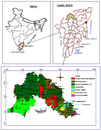
Figure 1.
Geology and sample location map of the study area.
The weathered zone thickness in the study area extends from <1 m to > 15 m. The yield of large diameter dug wells in the area ranges from 100 to 500 liters per minute (lpm), tapping the weathered layer of crystalline rocks. These wells are usually pumped for about 2 to 6 h a day, depending on the topography and weathered layer characteristics. The depth to the water level (DWL) throughout the pre-monsoon season stays within 0.5 and 9.9 m in below ground level (mbgl) in the district and the major part of the area has >5.5 mbgl. However, it stays within 2 and 9.9 mbgl throughout the post monsoon period. It can be generalized that the DTW in the study area ranges from 5–10 mbgl except for a few isolated pockets. Successful exploratory wells drilled in this region have a yield ranged between 0.78 liter per second (lps) and 26 lps. According to the earlier studies conducted by Central Groundwater Board (CGWB), the wells placed in granitic gneiss show higher yields than that of the wells placed within the Charnockites region. The specific capacity of various wells extents from 1.2 to a highest limit of 118.0 lpm/m/dd. The peizometric heads vary from 0.50 to 18.45 mbgl according to the thickness of the fracture zones.
3. Methods
A total of 39 groundwater samples were collected from different lithologies in the study area (Figure 1) and analyzed for various major ions and heavy metals. Prior to sampling, the sample bottles were rinsed with the sampled water. The collected samples were acidified by bringing the pH to ~2 with help of HNO3- and preserved at a temperature of 4 °C for metal analysis. Filtration was done with the use of a pre-conditioned plastic Millipore filter unit using a 0.45-μm filter membrane. pH, electrical conductivity (EC) and total dissolved solids (TDS) were measured in the field using portable meters (Thermo). Ca, Mg, Cl, HCO3 were analyzed by titrimetry; Na and K by Flame Photometer (Elico CL 378) and SO4 by Spectrophotometer (SL 171 minispec). The metal concentrations were determined in the samples by Inductively Coupled Plasma Mass Spectrometry (ICP-MS) (Model-ELAN DRC II, Perkin Elmer Sciex Instrument). Calibration was carried out to check the instrument drift. The National Institute of Standards and Technology Standard Reference Material (NIST-SRM) 1640 was adopted to minimize matrix and other interference effects along with the checking of the precision and accuracy of the analysis. Stable isotopes (Oxygen and Deuterium) present in the groundwater samples were analyzed using Isotopic Ratio Mass Spectrophotometer (Finnigan Deltaplus Xp, Thermo Electron Corporation, Bermen, Germany). The standard deviation of the measurements is ±1.72‰ for Oxygen and ±0.8‰ for Deuterium. All the measurements were carried out against laboratory substandard that were periodically calibrated against the international isotope water standards recommended by the IAEA (V-SMOW, GSIP and SLAP).
The isotope results obtained are reported in terms of δ units (Permil deviation of the isotope ratio from the international standard V-Smow) δ being defined by
where R = D/H or 18O/16O.
δ = [(Rsample − RSMOW/RSMOW)] × 103
4. Results
4.1. Hydrochemistry
The concentration of chemical constituents in groundwater is given in the box plot (Figure 2). pH is ranging from 6.5 to 8.1 with an average of 7.2, which indicate neutral to slightly alkaline in nature. EC values range from 602.1 to 1383.9 µs/cm with an average of 1010.4 µs/cm. Higher values were observed in SE and central parts of the study area (Figure 3). TDS ranging from 385.4 to 885.7 mg/L with an average of 646.6 mg/L and it follow the same trend of EC. Ca is the dominant cation followed by Na, Mg and K. Among the anions, Cl is the dominant ion followed by HCO3 and SO4. In the Piper plot [46], most of the samples represent Ca-Cl type (Figure 4), which indicate that the alkali earth exceeds the alkali and strong acid exceeds the weak acid. In the Gibbs plot [47], all the samples fall in the weathering dominance zone (Figure 5).
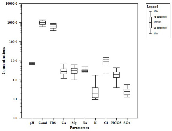
Figure 2.
Box plot for the chemical composition of groundwater (all values in mg/L, except pH and EC in µs/cm).
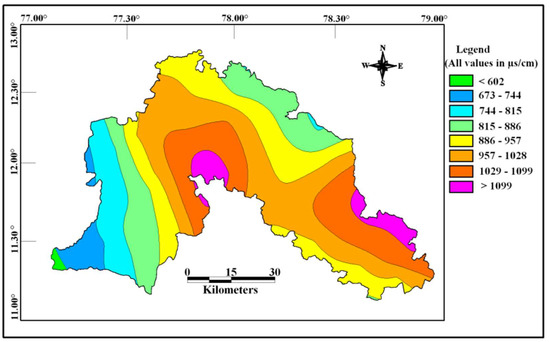
Figure 3.
Spatial distribution of EC in the study area.
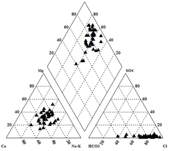
Figure 4.
Piper plot.
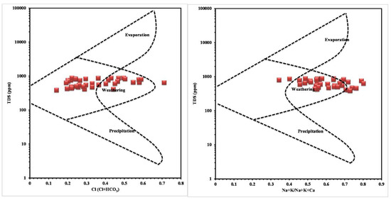
Figure 5.
Gibbs plot.
4.2. Heavy Metals
The concentration of heavy metals present in groundwater are shown in Table 1. The order of dominance of metals in groundwater is as follows: Zn> Ba> Sr> Fe> Al> B> Mn> Cu> Pb> Ni> V> Li> Rb> Cr> Mo> Se> As> Co> Cd> Ag> Sb> Be. The details of the individual metals are discussed below.

Table 1.
Trace metals concentration in groundwater of the study area (All values in ppb).
4.2.1. Aluminum (Al)
Aluminum is abundant in the earth’s crust. Few groundwater samples in the study area showing are above the permissible limit (200 ppb). Aluminum concentration in groundwater in most of the samples are within 200 ppb. Al ranges from 44.24 to 243.18 ppb along with a mean value of 151.80 ppb. 25% of the readings fall above the standard limits and 75% falls below the permissible limit.
4.2.2. Cadmium (Cd)
In the groundwater samples, Cd ranges from 0.09 to 0.36 ppb with a mean of 0.23 ppb and observed to be within the limit (5ppb) of WHO standard [48].
4.2.3. Lead (Pb)
The standard limit for the Pb in Groundwater is 0.5 ppb [49]. In the study area, it ranges from 3.60 ppb to 9.81 ppb with a mean value of 6.42 ppb. It is a matter of concern that that concentration of all the samples in the study area is above the permissible limit.
4.2.4. Zinc (Zn) and Copper (Cu)
In the study area, Zn limits varies from 333.44 ppb to 3267.50 ppb and has a mean value of 2049.87 ppb. The [48] recommended value for Zn is 3000 ppb. 10% of the water samples fall above the standard limit, whereas 90% of samples fall below the limit. Cu ranges from 3.92 to 11.02 ppb and has a mean value of 6.47 ppb. The permissible limit for Cu in groundwater is 2000 ppb [48]. Whereas, the majority of the samples are within the limit.
4.2.5. Selenium (Se)
In general, Selenium concentration in drinking water samples is strictly followed to be below the highest limit due to its toxicity. The Se ranges from 0.42 to 1.67 ppb with a mean value of 1.17 ppb in the study area. The permissible limit of the Se in groundwater is 50 ppb and it is observed that all the samples fall within the permissible limit.
4.2.6. Barium (Ba)
Barium in groundwater samples range from 28.48 to 684.80 ppb and has a mean value of 253.78 ppb. USEPA limit for Ba is 1000 ppb and all the samples in the study area are below the permissible limit.
4.2.7. Manganese (Mn)
In the study area, Mn ranges from 4.73 to 22.25 ppb and has a mean value of 14.61 ppb. World Health Organization (WHO) recommended limit of Mn is 300 ppb for drinking purpose [48] and all the samples fall within the standard limit.
4.2.8. Nickel (Ni) and Cobalt (Co)
The Ni and Co are common trace elements in basic rock and remain below 1000 ppb, are geochemically associated to Mn. The Ni concentrations in samples are between 2.41 and 9.67 ppb with a mean value of 6.16 ppb. Co ranges from 0.10 to 0.48 ppb and a mean value of 0.31 ppb. The recommended value for the Ni and Co in groundwater is 100 ppb and all samples fall below the permissible limit.
4.2.9. Arsenic (As)
As concentration in the study area ranges from 0.16 to 0.56 ppb and a mean value of 0.31 ppb. The permissible limit of As in groundwater is 10 ppb [48] and all the samples are at within the standard permissible levels.
4.2.10. Chromium (Cr)
In the study area, Cr ranges from 0.72 to 2.04 ppb and a mean value of 1.68 ppb. The [48] standard value for the Cr in groundwater is 50 ppb and all the samples are observed to be within the limit.
4.2.11. Molybdenum (Mo)
The concentration of the Mo in the study area ranges from 0.34 to 1.77 ppb and has a mean value of 0.70 ppb. The Permissible limit of Mo in groundwater is 10 ppb [50] and all the samples are within the limit.
4.2.12. Strontium (Sr)
Sr concentration in the study area ranges from 111.42 to 385.41 ppb and with a mean value of 225.67 ppb. The standard limit for Sr is 70 ppb [49] and it is observed that all the samples are above the permissible limit.
4.2.13. Boron (Br)
The concentration of the B ranges from 20.27 to 48.04 ppb with a mean value of 39.05 ppb. The permissible limit for B in groundwater is 300 ppb and values of all the samples fall below the permissible limit.
4.2.14. Iron (Fe)
The maximum permissible limit of Fe in public water supplies is 300 ppb. The concentration of Fe in the study area ranges from 47.87 to 244.46 ppb and a mean value of 144.67 ppb, which shows that all the samples are below the limits of permissible usage.
4.2.15. Lithium (Li) and Rubidium (Rb)
Feldspars and few clay minerals are the major sources of Lithium and Rubidium. The concentration of Li ranges from 0.54 to 5.36 ppb and has a mean value of 2.01 ppb. The Rb ranges from 0.30 to 2.28 ppb with a mean value of 0.81 ppb.
4.3. Stable Isotopes
25 groundwater samples were analyzed for stable isotopes (Oxygen and Hydrogen) during post monsoon period representing major lithologies in the study area. 11 groundwater samples from Quartzo feldspathic rocks, 6 samples from Epidote hornblende gneiss, 3 samples from Granite felsite/Pink migmatite, 1 sample from basic ultramafic rocks, 2 samples from Charnockite, 1 sample from Syenite complex and 1 sample from Amphibolite rock. The isotope results are given in δ units (per mil) from the international standard V-SMOW. Maximum, minimum and average values of isotopes for different lithologies are given in Table 2. Overall, the heavier (enriched) δ 18O value was recorded in epidote hornblende gneiss, and δD in granite felsite/pink migmatite.
Table 2.
Maximum, Minimum and Average values of δ18O and δD for different lithological unit (All values are in ‰).
5. Discussion
5.1. Major Ions
The order of dominance of ions are as follow: Cl > HCO3 > Ca > Na > Mg > K > SO4. Ca-Cl is the major water type in the study are, which indicates the dissolution of ions by the monsoonal rainfall recharge [51]. Gibbs plot also indicate the dominance of weathering process by the water-rock interaction through the recharge water [52]. Overall, the higher concentration of ions in groundwater at the discharge region (i.e. SE and the central parts of the study area) indicate the longer residence time of water in the aquifer [53].
5.2. Heavy Metals
Based on the heavy metal results, Sr, Ba, Al, Zn and Cu show high concentrations which are above the permissible limit. High intake of these metals can affect the cardiovascular system, bone development and metabolism in the human body and also cause dementia and carcinogen. The natural source of the heavy metal in groundwater are chiefly due to weathering of rock forming minerals present in the study area. The common metals present in these minerals are summarized in Table 3. Among all the alkali feldspars particularly Ba, Sr tends to co-dissolve with K+, Na+ and Ca2+ [54]. The clay minerals along with few other elements are presumed to be carried as well, which includes Mg2+. K-Feldspar is comparatively enhanced in Ba, Pb, Sr and Rb as compared to Na-feldspars [55], which indicate towards active weathering. The majority of these samples are found along with Al, which indicates the presence of aluminosilicates and this infers that pollution is not associated with agricultural impacts in this region. Ni, which is relatively enriched with clay is more mobile in slightly acidic aquatic mediums. Studies done by reference [56] have also recognized similar output and major relations with Mg2+, Ca2+ and Sr, and indicated pH as a dominant controlling factor. The increasing ion reduction and suggested co-dissolution with Fe, Co and Ni with a distinct relation and this desorption may be due to lowering of pH, with successive adsorption resulting due to higher pH [57].
Table 3.
Mineralogical compositions of sediments, mineral abundances, and estimated contribution to the chemical composition of the groundwater.
5.3. Factor Analysis
Factor analysis was used to identify the possible geochemical process which controls the ions and heavy metals and their relationship in the groundwater [58]. Totally seven factors were extracted with the cumulative percentage of 84.09 (Table 4). Factor 1 was loaded with Al, Cr, Mn, Fe, Ni, Co, Zn, Sr, Cd, Ba and Pb, which indicate the geogenic weathering of rocks within the aquifer system [59]. Mn oxide partially associated with Fe oxides as Fe-Mn oxyhydroxides in the sediments, where the Fe and Mn are the good scavengers of other metals [60].
Table 4.
Factor analysis.
Factor 2 was loaded with EC, TDS, Ca, Mg, Na and Cl which indicates the significant contribution of major ions to the overall groundwater chemistry. Each factor from 3 to 7 indicate the dissolution of minerals in the aquifer by the weathering process with less anthropogenic impacts. In general, the 1st factor was mostly controlled by the metals and the second factor by major ions in the groundwater chemistry.
5.4. Pollution Indices
The estimation of pollution indicators is usually determined to find the suitable utility of water for various purposes. The indices for the study including the heavy metal pollution index (HPI) and degree of contamination (Cd), are evaluated to determine the usage of water for drinking and agriculture purposes. Lower elemental concentrations than the permissible limits were not taken into consideration, because these metals do not pose any hazardous threat to the water quality. The HPI method has been used to obtain an overall quality of water specifically related to heavy metals. With the help of the analyzed value of metals, this method is evaluated considering the number of metals considered and their maximum allowable concentrations of the considered metals. In the Cd method, quality evaluation is done by computing the spanning of contamination. The Cd is calculated for each sample and is computed as the sum of the contamination factors of every component above the upper permissible limit. Hence the Cd summarizes the merged effects of a number of quality parameters considered to be unsafe for domestic water.
5.4.1. Heavy Metal Pollution Index
The heavy metal pollution index was created with the help of chosen variables along with the selection of pollution parameter on which the index was assigned a rating or weightage (Wi) for each parameter. The rating can be defined as the arbitrary value that stays between 0 and 1, whose selection shows the respective importance in the case of individual quality consideration. It is inversely proportional to the recommended standard (Si) for each parameter [61,62].
The maximum desirable value (li) for each parameter and the highest permissible value for drinking water (Si) were considered in this study based on the WHO standard. The highest permissible value for drinking water (Si) is shown to be the highest allowable limit in drinking water. The maximum desirable limit (li) shows the standard value permitted for drinking purpose.
The expression below [62] determines the HPI with the help of assigning a rating or weightage (Wi) for each of the parameter selected for this purpose.
Here, Wi and Qi represent the sub-index and unit weight of the ith parameter respectively, whereas n represents the number of parameters considered. The sub-index (Qi) is evaluated by
where Mi, Ii and Si represents the analyzed metal, it’s ideal value and the standard value of the ith parameter respectively. The sign (−) represents numerical difference between the two values and ignoring the algebraic sign.
The computation of the heavy metal pollution index was done by following the international standard [63]. HPI values ranges from 5.07 to 264.80 with a mean value of 132.33. The results show that the HPI values for 14 samples have lesser values compared to the critical limit of 100 for drinking standards [64].
5.4.2. Degree of Contamination
The contamination index (Cd) concludes the mixed effects of various quality parameters and contemplated unsafe to household water [64], and is evaluated as follows:
where
Cfi, CAi and CNi represent contamination factor, analytical value and upper permissible concentration of the ith component respectively, and N denotes the ‘normative value’. CNi is taken from maximum acceptable concentration (MAC).
The degree of contamination (Cd) was used as a standard to evaluate the extent of metal contamination in water [65]. The mean values of Cd are 115.79 and it ranges from 54.59 to 183.27, from which it is estimated that 54% of the samples have values under the mean value. Cd can be grouped into three categories, which are low (Cd < 1), medium (Cd = 1–3), and high (Cd > 3). In most of the samples, over the values exceed 3, which is an indication of high level of pollution. Therefore, Cd concentration categorizes all the samples as polluted, whereas HPI indicates that only part of the samples falls under polluted category. According to HPI, 64% of groundwater samples fall under the polluted category. Computation of the percentage deviations and mean deviation (Table 5) shows that HPI and Cd values are under their respective mean values. Furthermore, their related negative percentage of deviations points towards relative better quality of water, has also been distinguished previously by different authors [63,64].
Table 5.
Pollution indices for the groundwater samples.
In the present study, modified HPI and Cd were also done using the mean approach method [63] and the results are shown in Table 6. The value of HPI and Cd in the groundwater samples indicate 41% and 15% are classified as low, 56% and 82% are classified as medium, and 3% and 2% are classified under the highly polluted category respectively.
Table 6.
Classification of groundwater quality of the study area on modified categories of pollution indices.
In order to examine the contribution of metals to the computed indices, correlation analysis was done between the indices (Cd and HPI) and the heavy metal concentrations. As a result, Al-Cr-Mn-Fe-Ni-Co-Zn-Ba-Pb show good correlations with the indices, reveal the fact that these metals are the major contributors of pollution (Table 7). It also indicates the weathering of rock matrix is the dominant source of metals in the groundwater.
Table 7.
Correlation coefficients for metal concentrations and indices values.
Correlations seems to be very significant between the values of Cd and HPI. The indices values of Cd and HPI are presented on the spatial maps (Figure 6 and Figure 7). The Cd and HPI increases towards the northwest and western section of the study area. This region is covered with feldspathic gneiss and charnockites. The water level of this region is deeper and the rock type is less weathered, indicating a long residence time of water with less recharge. During weathering of plagioclase and clay minerals, trace and major elements releases with the help of an incongruent reaction and influences the composition of groundwater.
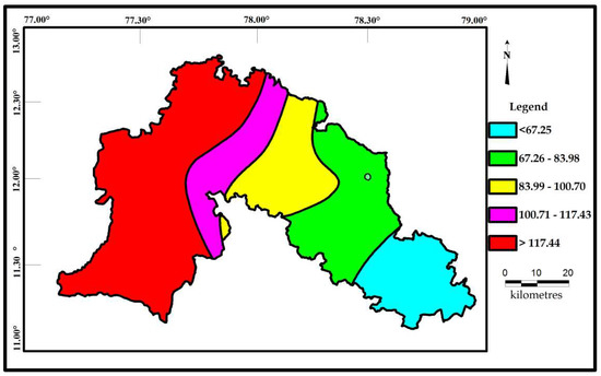
Figure 6.
Spatial distribution of Cd for the samples collected in the study area.
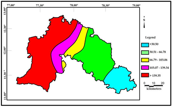
Figure 7.
Spatial distribution of HPI for the samples collected in the study area.
5.5. Isotope Signatures
5.5.1. Oxygen & Hydrogen
The isotopic data reveals that the isotopic variations are observed in different lithologies. Overall, the isotopic values of oxygen and hydrogen are higher in hornblende gneiss followed by Quartzo feldspathic rocks. δD and δ18O data provides information on the secondary processes acting on the water as it travels into the subsurface. The δD versus δ18O diagram (Figure 8) shows the groundwater data plot to the right of the GMWL [66]. Two clusters have been identified, in which Group A samples fall near the LMWL and parallel to the line, indicating that they are recharged by the local precipitation. Most of the groundwater samples have relatively depleted isotopic signatures (high negative values), which also indicates that the groundwater is recharged by the local precipitation. Group B samples deviate from the LMWL, indicating that these samples have undergone some evaporation prior to infiltration [67]. It is also noted that five samples in the study area (Hosur, Samalpatti, Hanumanthirtham, Anakodi and Thally) are relatively enriched with isotopes, indicating recharge from surface water or by evaporating water body [68].
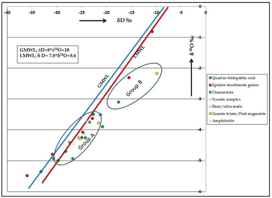
Figure 8.
Plot for δ18O versus δD.
The spatial distribution of δ18O in groundwater shows that the isotopically depleted groundwater samples occurs near northeast and northwest part of the study area and heavier isotopes in the south eastern part of the study area (Figure 9). Spatial variation of δD (Figure 10) showed that the region with lesser values are represented along the northeastern and western part, whereas heavier values are in the south as a small patch in the study area. It is interesting to observe a relative uniformity with minor variation in δ18O isotope composition in almost all the samples whose values range from −5.6 to −0.83 per mil and that of δD range from −36.1 and −9.8 per mil.
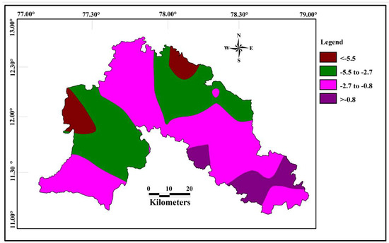
Figure 9.
Spatial distribution of δ 18O in the groundwater (in permil).
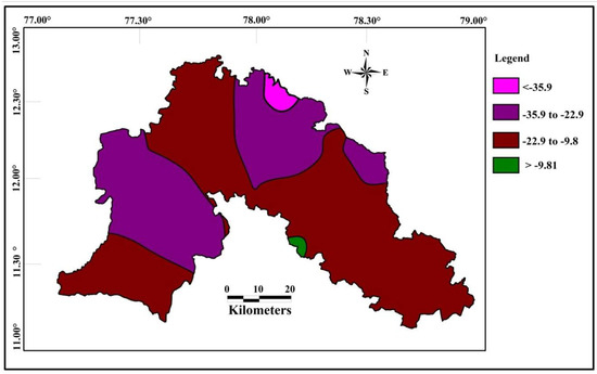
Figure 10.
Spatial distribution of δD in the groundwater (in permil).
Spatially both δ18O and δD are depleted along the same part of western and north eastern part of the study area. The western and north eastern part consist of hilly areas with higher altitudes, which indicate the influence of local precipitation on recharge. Heavier isotopes are noted along the south eastern part of the study area, with lesser elevation. The heavier isotopes in this part is mostly controlled by the evaporation of surface water body.
A comparison of the δ18O and chloride provides greater understanding of groundwater-surface water interaction processes in the study area. There is significant variation in the isotopic values with respect to Cl- concentration. The chloride- δ18O plot suggests that three types of groundwater occur in the study area (Figure 11.) namely: (i) Group A groundwater samples are characterized by low chloride and depleted δ18O representing the regions that are recharged frequently by rainfall [53]. (ii) Groundwater samples in Group B with high chloride and depleted δ18O, indicating that they rarely receive a recharge from meteoric water and are affected by minor anthropogenic activities. Higher concentration of chloride ion was attributed to the leaching of secondary salts present in the formation along the cracks and joints [69]. (iii) Group C samples show a higher concentration of chloride with enriched δ18O due to recharge from the evaporated water bodies or due to the evaporation taking place along the fractures or due to the diffusive recharge along the flow path [70].
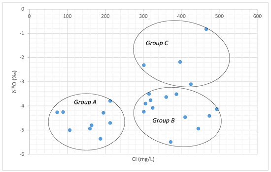
Figure 11.
Chloride vs. δ18O plot.
The chloride-deuterium plot also reflects the similar pattern characterized by high chloride and relatively enriched δD signatures in Group C samples (Figure 12), indicating recharge by evaporated water bodies [53]. Groundwater samples in Group B with high Cl− and depleted deuterium rarely receive recharge from meteoric water and may be recharged by the evaporated waters from a different source nearby or due to the evaporation taking place along the fractures in the aquifers. Group A is represented with low Cl− and depleted δD signatures show the recharge of local precipitation with less evaporated source.
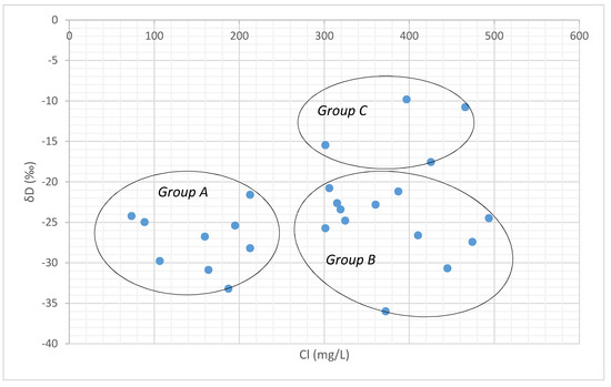
Figure 12.
Chloride vs. δD plot.
5.5.2. Deuterium Excess
The deuterium excess values are helpful to evaluate the origin of air masses from which precipitation resulted and they are also extensively used to identify the origin of vapor source [71]. If the d-excess values fall between 8% and 10‰, they indicate the primary precipitation and >10‰ represents the re-evaporation from the local surface water bodies under low humidity. The d-excess values for groundwater samples were calculated as [72]
d-excess = δD − 8x δ18O
Groundwater samples in the study area show d-excess values ranging from −4.2% to 12.76‰ and most of the samples fall below <10‰. It indicates the dominance of evaporation of rain water. Few samples are above 10‰, which could be the contribution from evaporation of local surface water. A plot of d-excess versus δ18O is given in Figure 13. From the plot, an inverse relation was observed between the d-excess and δ18O plots, which indicates the kinetic evaporation of surface water before recharging groundwater [70].
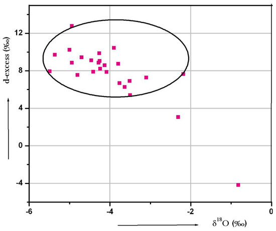
Figure 13.
Plot for d-excess versus δ18O.
6. Conclusions
The general chemistry of the groundwater indicates weathering and dissolution of ions through the local precipitation recharge. Trace metals results indicate that Sr and Ba in all the samples are greater than the permissible limit and few samples show Al, Zn and Cu are above the permissible limit and other metals analyzed are within the permissible limit. The higher concentration of these metals is inferred to be from geogenic sources, as the region is relatively free from industries. Based on HPI and Cd values in the groundwater, 41% and 15% of samples are considered as low, 56% and 82% as medium, and 3% and 2% are distinguished as being highly polluted. Al-Cr-Mn-Fe-Ni-Co-Zn-Ba-Pb show good correlations with the indices, which indicate that these metals are the major contributor to the water quality. Factor analysis indicates the weathering of rock matrix is the chief geochemical process to derive the metals into the groundwater with minimal anthropogenic impact. Isotopic signatures in the groundwater reveals that the recharge of the aquifers is mainly controlled by the precipitation and supported by evaporation of local surface water sources. Few metals are in an alarming concentration, which can cause risks to human health and the environment. So, there is a need for a sustainable management approach to treat the polluted water for sustainable usage.
Author Contributions
Data curation, S.M.; Formal analysis, S.C.; Investigation, S.C. and M.V.P.; Methodology, S.M.; Writing—original draft, S.C.; Writing—review & editing, M.V.P. and R.R.G.
Funding
This research was funded by Ministry of Environment and Forest (MoEF), India, 1-6/2007-CT dated 07.10.2009.
Acknowledgments
The authors thank the Jawaherlal Nehru University, New Delhi, India for the isotope analysis.
Conflicts of Interest
The authors declare no conflict of interest.
References
- Madhav, S.; Ahamad, A.; Kumar, A.; Kushawaha, J.; Singh, P.; Mishra, P.K. Geochemical assessment of groundwater quality for its suitability for drinking and irrigation purpose in rural areas of Sant Ravidas Nagar (Bhadohi), Uttar Pradesh. Geol. Ecol. Landsc. 2018, 2, 127–136. [Google Scholar] [CrossRef]
- Thilagavathi, R.; Chidambaram, S.; Thivya, C.; Prasanna, M.V.; Keesari, T.; Pethaperumal, S. Assessment of groundwater chemistry in layered coastal aquifers using multivariate statistical analysis. Sustain. Water Resour. Manag. 2017, 3, 55–69. [Google Scholar] [CrossRef]
- Devaraj, N.; Chidambaram, S.; Gantayat, R.R.; Thivya, C.; Thilagavathi, R.; Prasanna, M.V.; Panda, B.; Adithya, V.S.; Vasudevan, U.; Pradeep, K.; et al. An insight on the speciation and genetical imprint of bicarbonate ion in the groundwater along K/T boundary, South India. Arab. J. Geosci. 2018, 11, 291. [Google Scholar] [CrossRef]
- Rao1, K.N.; Latha, P.S. Groundwater quality assessment using water quality index with a special focus on vulnerable tribal region of Eastern Ghats hard rock terrain, Southern India. Arab. J. Geosci. 2019, 12, 267. [Google Scholar] [CrossRef]
- Jaishankar, M.; Tseten, T.; Anbalagan, N.; Mathew, B.B.; Beeregowda, K.N. Toxicity, mechanism and health effects of some heavy metals. Interdiscip. Toxicol. 2014, 7, 60–72. [Google Scholar] [CrossRef]
- Ritter, L.; Solomon, K.; Sibley, P.; Hall, K.; Keen, P.; Mattu, G.; Linton, B. Sources, pathways, and relative risks of contaminants in surface water and groundwater: A perspective prepared for the Walkerton inquiry. J. Toxicol. Environ. Health Part A 2002, 65, 1–142. [Google Scholar] [PubMed]
- Kungolos, A.; Samaras, P.; Tsiridis, V.; Petala, M.; Sakellaropoulos, G. Bioavailability and toxicity of heavy metals in the presence of natural organic matter. J. Environ. Sci. Health Part A 2006, 41, 1509–1517. [Google Scholar] [CrossRef]
- Jacob, J.M.; Karthik, C.; Saratale, R.G.; Kumar, S.S.; Prabakar, D.; Kadirvelu, K.; Pugazhendhi, A. Biological approaches to tackle heavy metal pollution: A survey of literature. J. Environ. Manag. 2018, 217, 56–70. [Google Scholar] [CrossRef]
- Abolude, D.S.; Davies, O.A.; Chia, A.M. Distribution and concentration of trace elements in Kubanni reservoir in Northern Nigeria. Res. J. Environ. Earth Sci. 2009, 1, 39–44. [Google Scholar]
- Okoya, A.A.; Asubiojo, O.I.; Amusan, A.A. Extractable metals and physicochemical properties of some Southwestern Nigerian Soils. In Biotechnology Development and Threat of Climate Change in Africa: The Case of Nigeria; Cuvillier Verlag: Gottingen, German, 2010; Volume 2, pp. 166–176. [Google Scholar]
- Sarma, G.K.; Gupta, S.S.; Bhattacharyya, K.G. Nanomaterials as versatile adsorbents for heavy metal ions in water: A review. Environ. Sci. Pollut. Res. 2019, 26, 6245–6278. [Google Scholar] [CrossRef]
- Bouhidel, K.-E.; Rumeau, M. Ion-exchange membrane fouling by boric acid in the electrodialysis of nickel electroplating rinsing waters: Generalization of our results. Desalination 2004, 167, 301–310. [Google Scholar] [CrossRef]
- Foster, I.D.L.; Charlesworth, S.M. Heavy metals in the hydrological cycle: Trends and explanation. Hydrol. Process. 1996, 10, 227–261. [Google Scholar] [CrossRef]
- Rainbow, P.S. Biomonitoring of heavy metal availability in the marine environment. Mar. Pollut. Bull. 1995, 31, 183–192. [Google Scholar] [CrossRef]
- Adriano, D.C. Trace Elements in Terrestrial Environments; Springer: New York, NY, USA, 2001; pp. 219–261. [Google Scholar]
- Rondeau, V.; Commenges, D.; Jacqmin-Gadda, H.; Dartigues, J.F. Relation between aluminum concentrations in drinking water and Alzheimer’s disease: An 8-year follow-up study. Am. J. Epidemiol. 2000, 152, 59–66. [Google Scholar] [CrossRef] [PubMed]
- Orisakwe, O.E.; Igwilo, I.O.; Afonne, O.J.; Maduabuchi, J.M.; Obi, E.; Nduka, J.C. Heavy metal hazards of sachet water in Nigeria. Arch. Environ. Occup. Health 2006, 61, 209–213. [Google Scholar] [CrossRef] [PubMed]
- Adepoju-Bello, A.A.; Alabi, O.M. Heavy metals: A review. Nig. J. Pharm 2005, 37, 41–45. [Google Scholar]
- Berman, E. Toxic Metals and Their Analysis; John Wiley & Sons: Hoboken, NJ, USA, 1980. [Google Scholar]
- Zietz, B.P.; Laß, J.; Suchenwirth, R. Assessment and management of tap water lead contamination in Lower Saxony, Germany. Int. J. Environ. Health Res. 2007, 17, 407–418. [Google Scholar] [CrossRef]
- Kojola, W.H.; Brenniman, G.R.; Carnow, B.W. A review of environmental characteristics and health effects of barium in public water supplies. Rev. Environ. Health 1979, 3, 79–95. [Google Scholar]
- Beaucaire, C.; Michard, G. Origin of dissolved minor elements (Li, Rb, Sr, Ba) in superficial waters in a granitic area. Geochem. J. 1982, 16, 247–258. [Google Scholar] [CrossRef]
- Zhang, H.; Zhou, X.; Wang, L.; Wang, W.; Xu, J. Concentrations and potential health risks of strontium in drinking water from Xi’an, Northwest China. Ecotoxicol. Environ. Saf. 2018, 164, 181–188. [Google Scholar] [CrossRef] [PubMed]
- Sankar, K.; Jagannath, B.; Sibasree, K. Boron Content in Shallow Ground Water of Andhra Pradesh and Telangana States, India. IOSR J. Environ. Sci. Toxicol. Food Technol. 2017, 11, 56–60. [Google Scholar] [CrossRef]
- Rout, G.R.; Sahoo, S. Role of iron in plant growth and metabolism. Rev. Agric. Sci. 2015, 3, 1–24. [Google Scholar] [CrossRef]
- Chidambaram, S.; Karmegam, U.; Prasanna, M.V.; Sasidhar, P.; Vasanthvigar, M. A study on hydrochemical elucidation of coastal groundwater in and around Kalpakkam region, Southern India. Environ. Earth Sci. 2011, 64, 1419–1431. [Google Scholar] [CrossRef]
- Chubaka, C.E.; Whiley, H.; Edwards, J.W.; Ross, K.E. Lead, Zinc, Copper, and Cadmium content of water from South Australian Rainwater Tanks. Int. J. Environ. Res. Public Health 2018, 15, 1551. [Google Scholar] [CrossRef]
- Prasanna, M.V.; Praveena, S.M.; Chidambaram, S.; Nagarajan, R.; Elayaraja, A. Evaluation of water quality pollution indices for heavy metal contamination monitoring: A case study from Curtin Lake, Miri City, East Malaysia. Environ. Earth Sci. 2012, 67, 1987–2001. [Google Scholar] [CrossRef]
- Halder, J.N.; Islam, M.N. Water pollution and its impact on the human health. J. Environ. Hum. 2015, 2, 36–46. [Google Scholar] [CrossRef]
- Tiwari, A.; Dwivedi, A.C.; Mayank, P. Time scale changes in the water quality of the Ganga River, India and estimation of suitability for exotic and hardy fishes. Hydrol. Curr. Res. 2016, 7, 254. [Google Scholar]
- Chaturvedi, A.; Bhattacharjee, S.; Singh, A.K.; Kumar, V. A new approach for indexing groundwater heavy metal pollution. Ecol. Indic. 2018, 87, 323–331. [Google Scholar] [CrossRef]
- Van Vliet, M.T.H.; Flörke, M.; Harrison, J.A.; Hofstra, N.; Keller, V.; Ludwig, F.; Spanier, J.E.; Wada, M.S.Y.; Wen, Y.; Williams, R.J. Model inter-comparison design for large-scale water quality models. Curr. Opin. Environ. Sustain. 2019, 36, 59–67. [Google Scholar] [CrossRef]
- Larsen, D.; Swihart, G.H.; Xiao, Y. Hydrochemistry and isotope composition of springs in the Tecopa basin, southeastern California, USA. Chem. Geol. 2001, 179, 17–35. [Google Scholar] [CrossRef]
- Yolcubal, I.; Gunduz, O.C.A.; Kurtulus, N. Origin of salinization and pollution sources and geochemical processes in urban coastal aquifer (Kocaeli, NW Turkey). Environ. Earth Sci. 2019, 78, 181. [Google Scholar] [CrossRef]
- Fernandes, P.; Carvalho, M.R.; Silva, M.C.; Rebelo, A.; Zeferino, J. Application of nitrogen and boron isotopes for tracing sources of anthropogenic contamination in Monforte-Alter do Chao aquifer system, Portugal. Sustain. Water Resour. Manag. 2019, 5, 249–266. [Google Scholar] [CrossRef]
- Kohfahl, C.; Rodriguez, M.; Fenk, C.; Menz, C.; Benavente, J.; Hubberten, H.; Meyer, H.; Paul, L.; Knappe, A.; López-Geta, J.A.; et al. Characterising flow regime and interrelation between surface-water and ground-water in the Fuente de Piedra salt lake basin by means of stable isotopes, hydrogeochemical and hydraulic data. J. Hydrol. 2008, 351, 170–187. [Google Scholar] [CrossRef]
- Oyarzún, J.; Núñez, J.; Fairley, J.P.; Tapia, S.; Alvarez, D.; Maturana, H.; Arumí, J.L.; Aguirre, E.; Carvajal, A.; Oyarzún, R. Groundwater Recharge Assessment in an Arid, Coastal, Middle Mountain Copper Mining District, Coquimbo Region, North-central Chile. Mine Water Environ. 2019. [Google Scholar] [CrossRef]
- Saltel, M.; Rebeix, R.; Thomas, B.; Franceschi, M.; Lavielle, B.; Bertran, P. Paleoclimate variations and impact on groundwater recharge in multi-layer aquifer systems using a multi-tracer approach (northern Aquitaine basin, France). Hydrogeol. J. 2018. [Google Scholar] [CrossRef]
- Kanduč, T.; Mori, N.; Kocman, D.; Stibilj, V.; Grassa, F. Hydrogeochemistry of alpine springs from North Slovenia: Insights from stable isotopes. Chem. Geol. 2012, 300–301, 40–54. [Google Scholar]
- Madlala, T.; Kanyerere, T.; Oberholster, P.; Xu, Y. Application of multi-method approach to assess groundwater–surface water interactions, for catchment management. Int. J. Environ. Sci. Technol. 2019, 16, 2215–2230. [Google Scholar] [CrossRef]
- Pu, T.; He, Y.; Zhang, T.; Wu, J.; Zhu, G.; Chang, L. Isotopic and geochemical evolution of ground and river waters in a karst dominated geological setting: A case study from Lijiang basin, South-Asia monsoon region. Appl. Geochem. 2013, 33, 199–212. [Google Scholar] [CrossRef]
- Apollaro, C.; Dotsika, E.; Marini, L.; Barca, D.; Bloise, A.; de Rosa, R.; Doveri, M.; Lelli, M.; Muto, F. Chemical and isotopic characterization of the thermo mineral water of Terme Sibarite springs (Northern Calabria, Italy). Geochem. J. 2012, 46, 117–129. [Google Scholar] [CrossRef]
- Vespasiano, G.; Apollaro, C.; de Rosa, R.; Larosa, F.M.S.; Fiebig, J.; Mulch, A.; Marini, L. The Small Spring Method (SSM) for the definition of stable isotope—Elevation relationships in Northern Calabria (Southern Italy). Appl. Geochem. 2015, 63, 333–346. [Google Scholar] [CrossRef]
- Manikandan, K.; Kannan, P.; Sankar, M. Evaluation and Management of Groundwater in Coastal Regions. Earth Sci. India 2012, 5, 1–11. [Google Scholar]
- Manikandan, K.; Natarajan, S.; Sivasamy, R.; Sankar, M.; Dadhwal, K.S. Spatial and Temporal Variation in Groundwater Characteristics of the Coastal Regions of Tamil Nadu. Indian For. 2011, 137, 1009–1014. [Google Scholar]
- Piper, A.M. A Graphic Procedure I the Geo-Chemical Interpretation of Water Analysis; US Geological Survey Groundwater: Washington, DC, USA, 1953; p. 63.
- Gibbs, R.J. Mechanisms controlling world water chemistry. Sci. J. 1970, 170, 795–840. [Google Scholar] [CrossRef]
- World Health Organization (WHO). Guidelines for Drinking-Water Quality; World Health Organization: Geneva, Switzerland, 2004; Volume 1. [Google Scholar]
- World Health Organization (WHO). Guidelines for Drinking Water Quality, 2nd ed.; World Health Organization: Geneva, Switzerland, 1998; p. 36. ISBN 9241545143. [Google Scholar]
- WHO. Guidelines for Drinking-Water Quality; World Health Organization: Geneva, Switzerland, 2011; Volume 216, pp. 303–304. [Google Scholar]
- Prasanna, M.V.; Nagarajan, R.; Chidambaram, S.; Kumar, A.A.; Thivya, C. Evaluation of hydrogeochemical characteristics and the impact of weathering in seepage water collected within the sedimentary formation. Acta Geochim. 2017, 36, 44–51. [Google Scholar] [CrossRef]
- Chidambaram, S.; Sarathidasan, J.; Srinivasamoorthy, K.; Thivya, C.; Thilagavathi, R.; Prasanna, M.V.; Singaraja, C. Assessment of hydrogeochemical status of groundwater in a coastal region of Southeast coast of India. Appl. Water Sci. 2018, 8, 27. [Google Scholar] [CrossRef]
- Prasanna, M.V.; Chidambaram, S.; Hameed, A.S.; Srinivasamoorthy, K. Study of evaluation of groundwater in Gadilam Basin using hydrogeochemical and isotope data. Environ. Monit. Assess. 2010, 168, 63–90. [Google Scholar] [CrossRef]
- Veer, G. Geochemical Soil Survey of The Netherlands. Atlas of Major and Trace Elements in Topsoil and Parent Material; Assessment of Natural and Anthropegenic Enrichment Factors; No. 347; Utrecht University: Utrecht, The Netherlands, 2006. [Google Scholar]
- Nagasawa, H.; Schnetzler, C.C. Partitioning of rare earth, alkali and alkaline earth elements between phenocrysts and acidic igneous magma. Geochim. Cosmochim. Acta 1971, 35, 953–968. [Google Scholar] [CrossRef]
- Navrátil, T.; Skřivan, P.; Minařík, L.; ŽIgová, A. Beryllium geochemistry in the Lesni potok catchment (Czech Republic), 7 years of systematic study. Aquat. Geochem. 2002, 8, 121–133. [Google Scholar] [CrossRef]
- Kjøller, C.; Postma, D.; Larsen, F. Groundwater acidification and the mobilization of trace metals in a sandy aquifer. Environ. Sci. Technol. 2004, 38, 2829–2835. [Google Scholar] [CrossRef]
- Prasanna, M.V.; Chidambaram, S.; Srinivasamoorthy, K. Statistical analysis of the hydrogeochemical evolution of groundwater in hard and sedimentary aquifers system of Gadilam river basin, South India. J. King Saud Univ. (Sci.) 2010, 22, 133–145. [Google Scholar] [CrossRef]
- Chidambaram, S.; Prasad, M.B.K.; Prasanna, M.V.; Manivannan, R.; Anandhan, P. Evaluation of metal pollution in groundwater in the industrialized environs in and around Dindigul, Tamilnadu, India. Water Qual. Expo. Health 2015, 7, 307–317. [Google Scholar] [CrossRef]
- Singh, S.K.; Subramanian, V.; Gibbs, R.J. Hydrous FE and MN oxides—Scavengers of heavy metals in the aquatic environment. Crit. Rev. Environ. Control 1984, 14, 33–90. [Google Scholar] [CrossRef]
- Trivedy, R.K. Encyclopedia of environmental pollution and control. Environ. Media 1995, 1, 342. [Google Scholar]
- Mohan, S.V.; Nithila, P.; Reddy, S.J. Estimation of heavy metals in drinking water and development of heavy metal pollution index. J. Environ. Sci. Health Part A 1996, 31, 283–289. [Google Scholar] [CrossRef]
- Edet, A.E.; Offiong, O.E. Evaluation of water quality pollution indices for heavy metal contamination monitoring. A study case from Akpabuyo-Odukpani area, Lower Cross River Basin (southeastern Nigeria). GeoJournal 2002, 57, 295–304. [Google Scholar] [CrossRef]
- Prasad, B.; Bose, J. Evaluation of the heavy metal pollution index for surface and spring water near a limestone mining area of the lower Himalayas. Environ. Geol. 2001, 41, 183–188. [Google Scholar] [CrossRef]
- Al-Ani, M.Y.; Al-Nakib, S.M.; Ritha, N.M.; Nouri, A.H. Water quality index applied to the classification and zoning of Al-Jaysh canal, Baghdad–Iraq. J. Environ. Sci. Health Part A 1987, 22, 305–319. [Google Scholar] [CrossRef]
- Craig, H. Isotopic variations in meteoric waters. Science 1961, 133, 1702–1703. [Google Scholar] [CrossRef] [PubMed]
- Baskaran, S.; Ransley, T.; Brodie, R.S.; Baker, P. Investigating groundwater–river interactions using environmental tracers. Aust. J. Earth Sci. 2009, 56, 13–19. [Google Scholar] [CrossRef]
- Simpson, H.J.; Herczeg, A. Salinity and evaporation in the river Murray River basin, Australia. J. Hydrol. 1991, 124, 1–27. [Google Scholar] [CrossRef]
- Chidambaram, S.; Ramanathan, A.L.; Prasanna, M.V.; Anandhan, P.; Srinivasamoorthy, K.; Vasudevan, S. Identification of hydrogeochemically active regimes in groundwaters of Erode district, Tamilnadu—A statistical approach. Asian J. Water Environ. Pollut. 2007, 5, 93–102. [Google Scholar]
- Thivya, C.; Chidambaram, S.; Rao, M.S.; Gopalakrishnan, M.; Thilagavathi, R.; Prasanna, M.V.; Nepolian, M. Identification of recharge processes in groundwater in hard rock aquifers of Madurai district using stable isotopes. Environ. Process. 2016, 3, 463–477. [Google Scholar] [CrossRef]
- Deshpande, R.D.; Bhattacharya, S.K.; Jani, R.A.; Gupta, S.K. Distribution of oxygen and hydrogen isotopes in shallow groundwaters from Southern India: Influence of a dual monsoon system. J. Hydrol. 2003, 271, 226–239. [Google Scholar] [CrossRef]
- Dansgaard, W. Stable isotopes in precipitation. Tellus 1964, 16, 436–468. [Google Scholar] [CrossRef]


© 2019 by the authors. Licensee MDPI, Basel, Switzerland. This article is an open access article distributed under the terms and conditions of the Creative Commons Attribution (CC BY) license (http://creativecommons.org/licenses/by/4.0/).