Atmospheric Control of Deep Chlorophyll Maximum Development

Abstract

The evolution of the near-surface phytoplankton bloom towards a Deep Chlorophyll Maximum (DCM) in mid-latitudes and subpolar regions of the global ocean is a well-known biological feature. However, our knowledge about the exact mechanism that determines the end of the bloom and its irreversible evolution towards a DCM is still limited. In this work, combining satellite and in-situ oceanographic data together with reanalysis data, we investigate why and when this transition between the near-surface phytoplankton bloom and the development of a DCM occurs. For this aim, we investigate the links between changes in air-sea heat exchanges, the near-surface signature of phytoplankton bloom, and the water column vertical structure by calculating the mixed layer depth (MLD) and depth of the DCM on hydrographic and chlorophyll profiles. We find that the occurrence of the last convective mixing event (heat loss by the ocean surface) at the end of the spring which is able to reach the base of the MLD and inject new nutrients into the mixed layer marks the end of the near-surface bloom and its transition towards a DCM. Identified in this way, the spring bloom duration and the start of the transition towards a DCM can be systematically and objectively determined, providing sensitive indexes of climate and ecosystem variability.

1. Introduction

In mid-latitude, subpolar, and polar regions, phytoplankton growth and biomass exhibit a marked seasonal cycle. The “critical depth” theory proposes that after winter mixing restores the nutrient content in the mixed layer, blooms commence when the ocean surface mixed-layer restratifies [1]. More accurately, the onset of the spring bloom can be identified when air-sea heat fluxes become positive (heat gain by the ocean surface), allowing incipient stratification to be established at the ocean surface along with phytoplankton growth [2,3], although this classical approach has been challenged by Behrenfeld [4]. Quickly (days–weeks), phytoplankton depletes nutrients in the well-illuminated mixed layer, becoming less abundant in the near-surface layer and accumulating at depth [5]. This process leads to the formation of persistent layers of elevated chlorophyll a concentrations, coinciding with the nutricline, which are nearly ubiquitous in stratified surface waters. These deep layers of elevated Chl are known as the Deep Chlorophyll Maximum (DCM) and the typical water column vertical structure of these regions have been characterized as the “Typical Tropical Structure” (TTS) by Herbland & Voituriez [6]. However, the TTS pattern is not exclusive to the tropics, however rather is observable in all waters that remain stable long enough for the development of a DCM. Accordingly, as proposed by Cullen [7], the term Typical Stable Water Structure (TSWS) seems more appropriate than TTS.

Both the importance of biomass accumulation associated with near-surface phytoplankton blooms and DCM have been largely recognized as ecological hot spots, determinant in the population dynamics of higher trophic levels and in global biogeochemical cycles [8,9]. Changes in bloom phenology have been reported as having potential catastrophic implications for higher trophic levels ([9] and references therein). Accordingly, they have been extensively studied, particularly with regard to changes in the onset of the spring bloom. However, the mechanisms that at some point make the bloom evolve irremediably towards a DCM have remained barely studied. Commonly, as noticed from what was put forth earlier, it is considered that quickly (days–weeks), phytoplankton depletes nutrients in the well-illuminated mixed layer concentrating at depth. Thus, our knowledge about the timing surrounding when the near surface bloom ends definitively and evolving irreversibly towards a DCM is only approximate.

In this work, combining satellite and in-situ oceanographic data together with reanalysis data, we investigate why and when the near-surface phytoplankton bloom evolves irremediably towards a DCM. The results of this investigation may allow the systematic and objective determination of spring bloom duration and the start of the transition towards a DCM, providing sensitive indexes of climate and ecosystem variability.

2. Materials and Methods

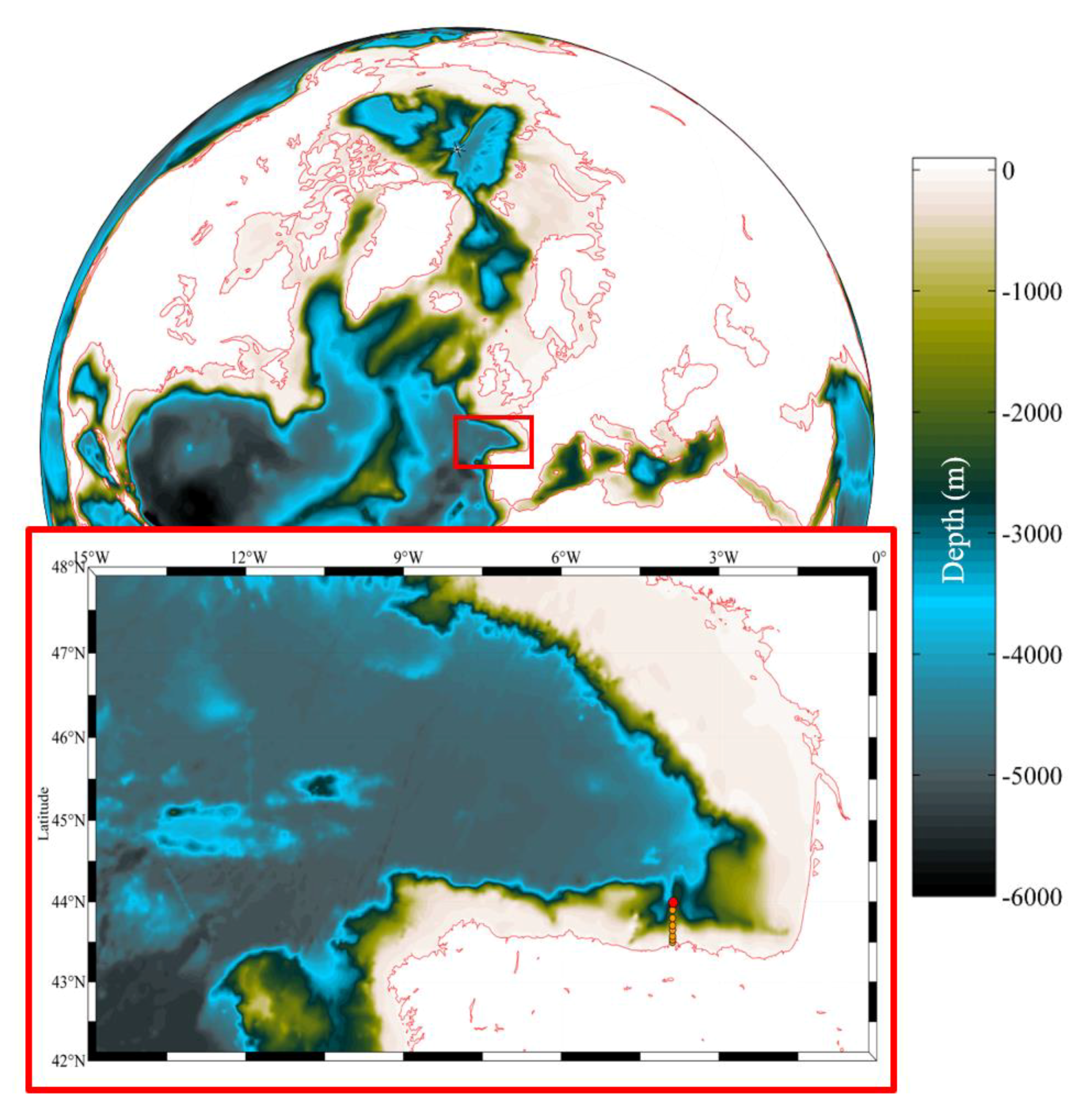
2.1. Study Area and Data Sources

The study focuses on the determination of the causes and timing of the transition between the end of the near-surface phytoplankton bloom and the development of a DCM that occurs in mid-latitudes and subpolar regions of the global ocean. For this aim, we will make use of the data of the long-term oceanographic time series at ocean observatory Santander Atlantic-Time-Series (SATS). These data are particularly suitable for this study because: (1) SATS is located at mid-latitudes (Figure 1); and (2) SATS data include the measurements of an oceanic-meteorological buoy (AGL buoy) equipped with oceanographic and biogeochemical sensors and its associated oceanographic station. The AGL buoy was deployed in 2007 by the Spanish Institute of Oceanography (IEO) at 2800 m depth in the Southern Bay of Biscay (43.8° N, 3.8° W) and, since then, it provides hourly data of the main atmospheric, oceanographic, and biogeochemical parameters as air pressure and temperature; relative humidity, wind direction, and speed (at a 2 m height); sea surface temperature (SST) and salinity (SSS); and dissolved oxygen and chlorophyll (at 3 m depth). Its mooring position was chosen to coincide with the ship-based monthly hydrographic and biogeochemical sampling of the Santander standard section running since 1991 by the IEO. The oceanographic station associated with the AGL buoy has been sampled since 1994. In each monthly sampling, hydrographic and biogeochemical parameters, such as temperature, salinity, chlorophyll, and oxygen, are measured by a CTD and water samples are taken for salinity, oxygen, and chlorophyll determinations. Thus, SATS data provides high-frequency repeated observations of interlinked meteorological, oceanographic, and biogeochemical variables that enable obtaining a comprehensive description of ocean processes from the seafloor to the atmosphere at a site that is representative of the mid-latitudes of the Eastern North Atlantic [10,11,12,13,14].

2.2. Changes in Air-Sea Exchanges, Near-Surface Chlorophyll, Depth of DCM, and Mixed-Layer Depth

As previously mentioned, the onset of the spring bloom can be accurately identified based on the moment at which the net heat flux from the ocean to the atmosphere becomes positive (ocean heat gain) and incipient stratification is established at the ocean surface [2,3]. The resulting water column stability allows at that moment bursts in phytoplankton biomass and its bloom. Similarly, the presence of a DCM is linked to waters that remain stable long enough for its development. Such stability requires the absence of mixing deep enough to reach the base of the mixed layer depth (MLD) and to provoke the erosion of the seasonal pycnocline. In view of that, we investigated the link between changes in air–sea heat exchanges, the heat storage in the water column, the water column vertical structure (MLD), and the transition between the near-surface phytoplankton bloom and the development of a DCM.

To assess changes in air–sea heat exchanges, we calculated the net heat flux from the ocean to the atmosphere (Q₀), which is given by the sum of four components: Q_E, the latent heat flux; Q_H, the sensible heat flux; Q_lw, the net longwave radiation flux; and Q_sw, the net shortwave radiation flux (solar radiation) (Figure 2). Q_lw and Q_sw (radiative heat fluxes) can be obtained from the NCEP/NCAR reanalysis data set [15] as daily values with a spatial resolution of 1.9° × 1.9°. Q_E and Q_H (turbulent heat fluxes) can be computed from atmospheric and oceanic AGL buoy measurements using the so-called bulk formulae (see [16] for further information). In this case, we used the Fairall algorithm [17], which is one of the most popular algorithms based on the bulk formulae, to compute turbulent heat fluxes from AGL buoy data.

The suitability of the use of alternative reanalysis data from e.g., ECMWF (https://www.ecmwf.int/) and OAFLUX project (http://oaflux.whoi.edu/) [18] have also been considered. Regarding the use of ECMWF reanalysis data, previous analyses have shown us limited sensitivity of the upper ocean response both e.g., in terms of SST or MLD variability to variation of atmospheric forcing reanalysis used for its investigation (NCEP/NCAR versus ECMWF) [12,14]. Thus, we do not repeat these sensitivity analyses here and refer the reader to these manuscripts [12,14]. On the other hand, OAFLUX project provides global time series of daily ocean latent and sensible heat fluxes at 1° × 1° spatial resolution combined with existing radiative heat flux products from ISCCP on OAFLUX grids. Radiative heat fluxes time-series provided by OAFLUX project ends in December 2009. Thus, their use for comparison with AGL buoy data starting in June 2007 is discarded, since they provide a short time-series for comparison. OAFLUX turbulent heat fluxes continue to present and have been compared with those provided by NCEP/NCAR reanalysis and estimated from AGL buoy data (Figure 3). As expected, it is observed how NCEP/NCAR reanalysis overestimates heat fluxes for large heat loss events (heat loss by the ocean surface is shown as positive values) [15]. However, in general, the cluster dispersion from OAFLUX data with respect to AGL buoy estimations is larger than from NCEP/NCAR reanalysis. Moreover, for the time period of the year of interest—between April and May—in this study, the mean values of Q_E(Q_H) vary between 50.16 ± 40.87 (5.74 ± 11.49) W·m⁻² estimated from AGL buoy data; 52.52 ± 46.56 (8.79 ± 14.39) W·m⁻² obtained from NCEP/NCAR reanalysis; and 48.03 ± 31.41 (10.60 ± 14.23) W·m⁻² from the OAFLUX project. Since large heat loss events overestimated by NCEP/NCAR Reanalysis are not the focus of this work, NCEP/NCAR Reanalysis data set shows better agreement with the AGL buoy heat flux estimations for the time-period of interest in this study. Thus, they are the only reanalysis data used hereinafter in this paper.

As mentioned, the transition from a near-surface phytoplankton bloom and development of a DCM requires the absence of mixing deep enough to reach the base of the mixed layer depth (MLD). To reach the MLD, heat loss events must be sufficiently negative to remove the accumulated heat above the MLD at that moment. Thus, to evaluate when these heat loss events take place, we calculate the time-series of heat storage (Q_strg) in the water column from hydrographic profiles from SATS oceanographic station as: Q_strg = ρ·C_p·h· δTa/δt, where ρ is the seawater density; Cp, the heat capacity of seawater; h, the depth determining the vertical extension of the mixed layer (MLD); and δTa/δt, the temporal evolution of the integrated temperature in the water column (Ta = $\frac{1}{h}{{\displaystyle \int }}_{-h}^{0}T\left(z\right)dz)$ (for further details, see [19,20]).

To identify the near-surface signal of the phytoplankton bloom, weekly and daily satellite-derived chlorophyll a concentration data provided by the GlobColour project (http://www.globcolour.info/) were used in combination with in-situ hourly chlorophyll concentration measurements provided by the AGL buoy. To evaluate the transition from the near-surface phytoplankton bloom towards a DCM and its relationship with the water column vertical structure, we employed fluorescence (chlorophyll) and density profiles from the SATS oceanographic station. For each chlorophyll profile, we estimate the depth of its chlorophyll maximum as the depth where the corresponding 5 m low-pass filter profile shows the maximum chlorophyll value as depicted in Figure 4. Chlorophyll is considered a proxy of phytoplankton biomass and so the depth of the chlorophyll maximum is the depth featuring the highest phytoplankton biomass. For each density profile, the MLD was obtained by applying the Gonzalez-Pola et al. [21] algorithm. Alternative estimates are not included in this work as robust performance of this algorithm and its comparison with other MLD determination methods have already been discussed in Somavilla et al. [14].

3. Results and Discussion

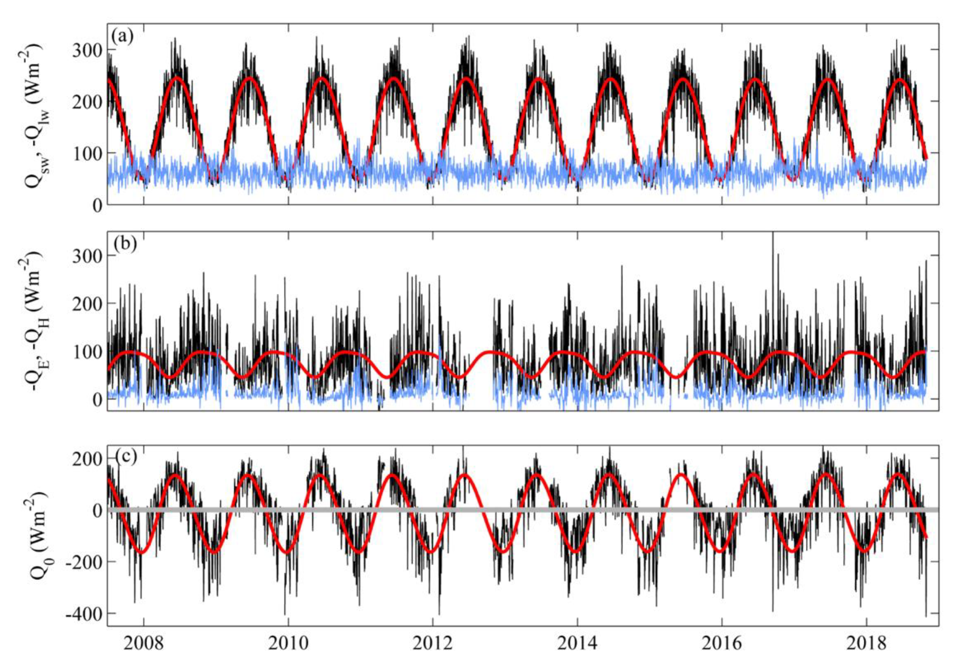
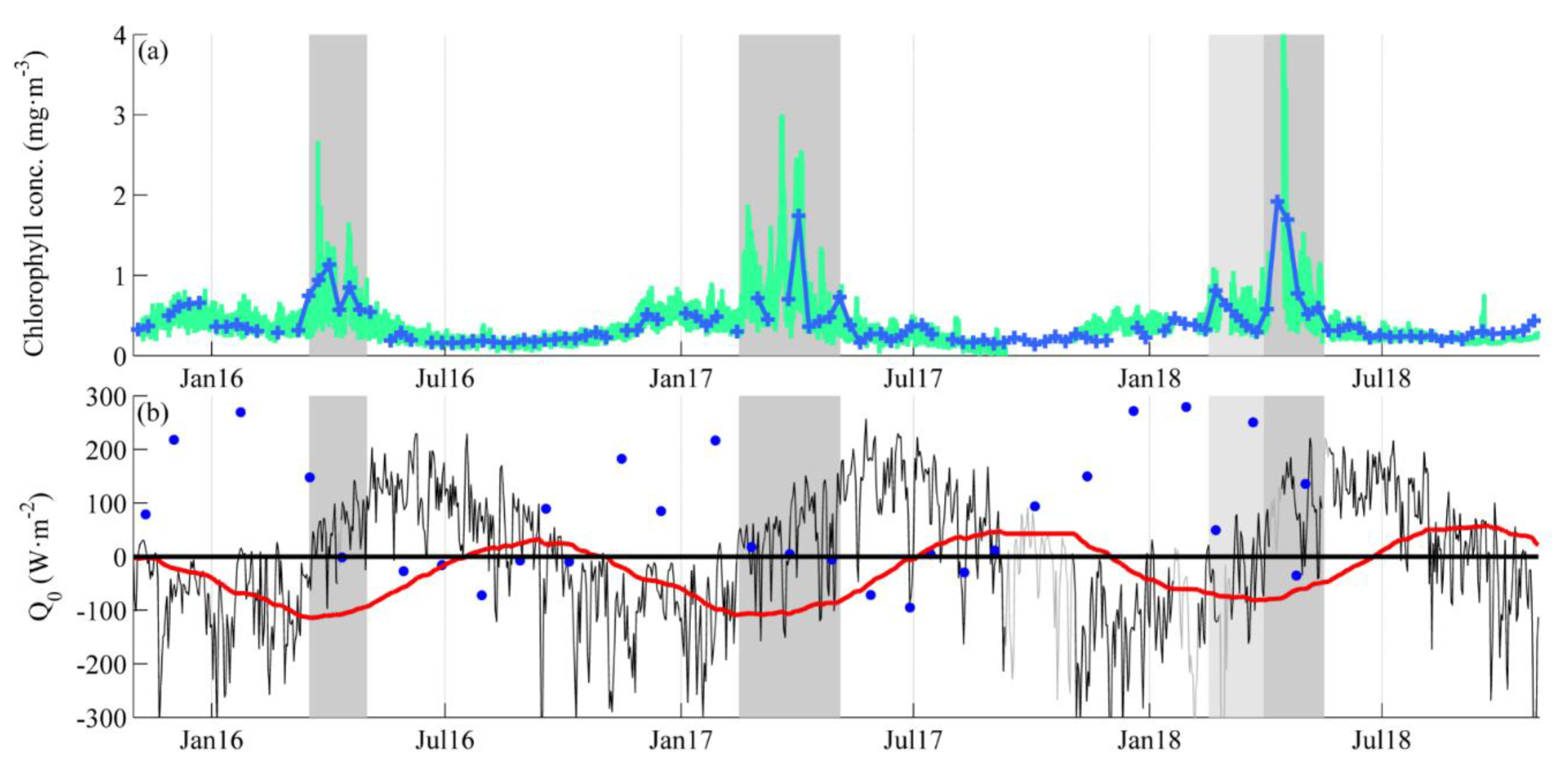
3.1. Near-Surface Phytoplankton Growth Signature and Changes in Air-Sea Exchanges

The near-surface chlorophyll concentration and Q₀ time-series (Figure 5) clearly show the reported link between the onset of the spring and Q₀ seasonal cycle. Bursts in phytoplankton biomass illustrated by the increase of near-surface chlorophyll concentration (Figure 5a) start every year when Q₀ passes initially from negative to positive values (Figure 5b; beginning of the grey shadow areas). At that moment, Q₀ passes from being a heat loss to a heat gain by the ocean surface (Q₀ changes from negative to positive values and the accumulated net heat flux reaches its minimum and starts to increase), indicating the beginning of spring warming and early stratification, thereby allowing phytoplankton growth [2,3]. Indeed, it is the marked Q₀ seasonal cycle oscillating within zero and so, between net heat gains and losses by the ocean surface, that tends to stabilize or destabilize the water column which drives not only the onset of the spring bloom, however, in general, the marked seasonal cycle in near-surface chlorophyll concentration. Thus, in order to facilitate the comprehension of the atmospheric control of the deep chlorophyll maximum development, it is convenient to remark on the drivers of Q₀ and mixing seasonal cycles.

Typically, at mid and high latitudes, solar radiation (net short-wave radiation flux, Q_sw) is the only component of the net heat flux between the ocean and atmosphere that represents a heat gain by the ocean (Figure 2a). The rest of the components extract heat from the ocean most of the time, experiencing small variations throughout the year (Figure 2a,b). On the other hand, Q_sw features a high amplitude seasonal cycle (195 W·m⁻²) that modulates the marked Q₀ annual cycle oscillating within zero. Q_E also shows a marked seasonal cycle although smaller in amplitude (52 W·m⁻²). Hence, during winter months, solar radiation is at its minimum and Q_sw and Q_lw, having opposite signs, tend to compensate one another (Figure 2a). Thus, their contribution to Q₀ is very small, however owing to the contribution of turbulent heat fluxes, Q_E and Q_H, Q₀ is negative and surface waters lose heat. Destabilizing buoyancy forcing from cooling (Q₀ < 0) making the ocean surface colder induces convective mixing of surface water with deeper water and controls the autumn–winter mixed layer deepening [12,23,24].

During spring and summer, Q_sw can be much higher than the sum of the remaining heat-loss terms (Figure 2). When Q₀ is positive, surface waters gain heat. Such heating—causing the ocean surface to become warmer—represents a stabilizing buoyancy, forcing stratification of the surface and isolating it from deeper waters [25]. However, between the end of the winter and late spring, Q₀ is not yet permanently positive and alternates with negative values (destabilizing) that can cause mixing to reach relatively deep values. After this period of alternation of convective mixing events (Q₀ < 0), stabilizing buoyancy forcing (Q₀ > 0) hinders upper ocean mixing and during the summer months, the vertical extension of the mixed layer is controlled by wind stress-induced mixing [12,14,23,24]. Such pure mechanical mixing is not as effective as convection to deepen the surface layer and MLD remains more or less stable during late spring and summer while Q₀ > 0 (Figure 5a,b). It is not until Q₀ is negative again (dark blue dashed line in Figure 5a) and so convective mixing is possible such that the mixed layer begins to thicken again in autumn and winter (Figure 5a,b).

With all that in mind, considering that the presence of a DCM is linked to waters that remain stable long enough for its development, the transition from the near-surface phytoplankton bloom towards a DCM could be established at the moment the last convective mixing episode that is able to reach the base of the MLD takes place in spring. To reach the MLD, Q₀ must be strong enough to remove the accumulated heat above the MLD at that moment shown by Q_strg in Figure 5b. Driven by negative Q₀ values in late spring, these last convective mixing events are highlighted in Figure 5b by the end of the grey shadow areas. They coincide every year with a last peak of the near-surface chlorophyll concentration and a drastic reduction afterwards. We interpret this as indicative of the end of the near-surface phytoplankton bloom and its transition towards a DCM.

Figure 5 shows data only from November 2015. A new chlorophyll sensor equipped with a bio-wiper that only exposes the instrument’s optical surface to the water during the time of the measurement (Wet Labs ECO Fluorometer FLS) was installed in the AGL buoy at that moment, showing very good performance. Previously, the sensors installed were largely affected by biofouling and the resulting chlorophyll time-series was useless. In order to provide higher confidence to the findings at the AGL buoy position, Figure 6 shows chlorophyll and Q₀ time-series at other locations in the mid-latitudes of the Eastern North Atlantic. It is also observed how at the different locations and for the different years the onset of the spring bloom coincides with the moment at which Q₀ passes from negative to positive values. In case later convective mixing events (Q₀ < 0) occur after the onset of the spring bloom, they resulted in additional peaks of the near near-surface chlorophyll concentration (or prolong the bloom duration). In the extreme case that there is no convective mixing event after the onset of the spring bloom (e.g., year 2016 at 46.67° N, 5.62° W; 44.76° N, 9.38° W; and 42.86° N, 11.25° W (Figure 6b–d)), the average bloom duration is ~40 days. The higher the number of alternation of stabilizing/destabilizing buoyancy events (positive/negative Q₀) after the onset of the spring bloom, the longer the duration of the bloom (e.g., the bloom duration in 2015 at the different locations shown in Figure 6 is approximately 85 days). For the years represented in Figure 5, the dates when the transition towards the DCM occurs vary between 29th April and 17th May. Considering them together with the dates establishing the onset of the bloom (varying between 15th February and 31st March), they imply that the duration of the bloom varies between 46 and 81 days. Thus, in general, the maximum duration of the bloom can even double the minimum. It brings to light how rough the common approximation is to consider that quickly phytoplankton depletes the nutrients in the well-illuminated mixed layer, becoming less abundant in the near-surface layer and concentrating at depth. On one hand, this implies that any estimate derived from a time integration of the bloom intensity could be affected by large biases. On the other hand, it questions the proposed mechanism primarily controlling the bloom duration. Just a “quick” nutrient consumption by the typical phytoplankton assemblage present at the beginning of the spring in the area cannot explain the almost doubling of bloom duration. In other words, the doubling of the bloom duration can only be explained by consecutive convective mixing episodes that are able to entrain additional nutrients into the mixed layer. It is the occurrence of the last convective mixing event driven by negative Q₀ that determines the last nutrient entrainment into the mixed layer, thereby sustaining an increase of the near-surface chlorophyll concentration (Figure 5a). From then onwards, the near-surface chlorophyll decreases irreversibly, not increasing again until the following winter, indicating the end of the near-surface bloom and the transition towards a DCM.

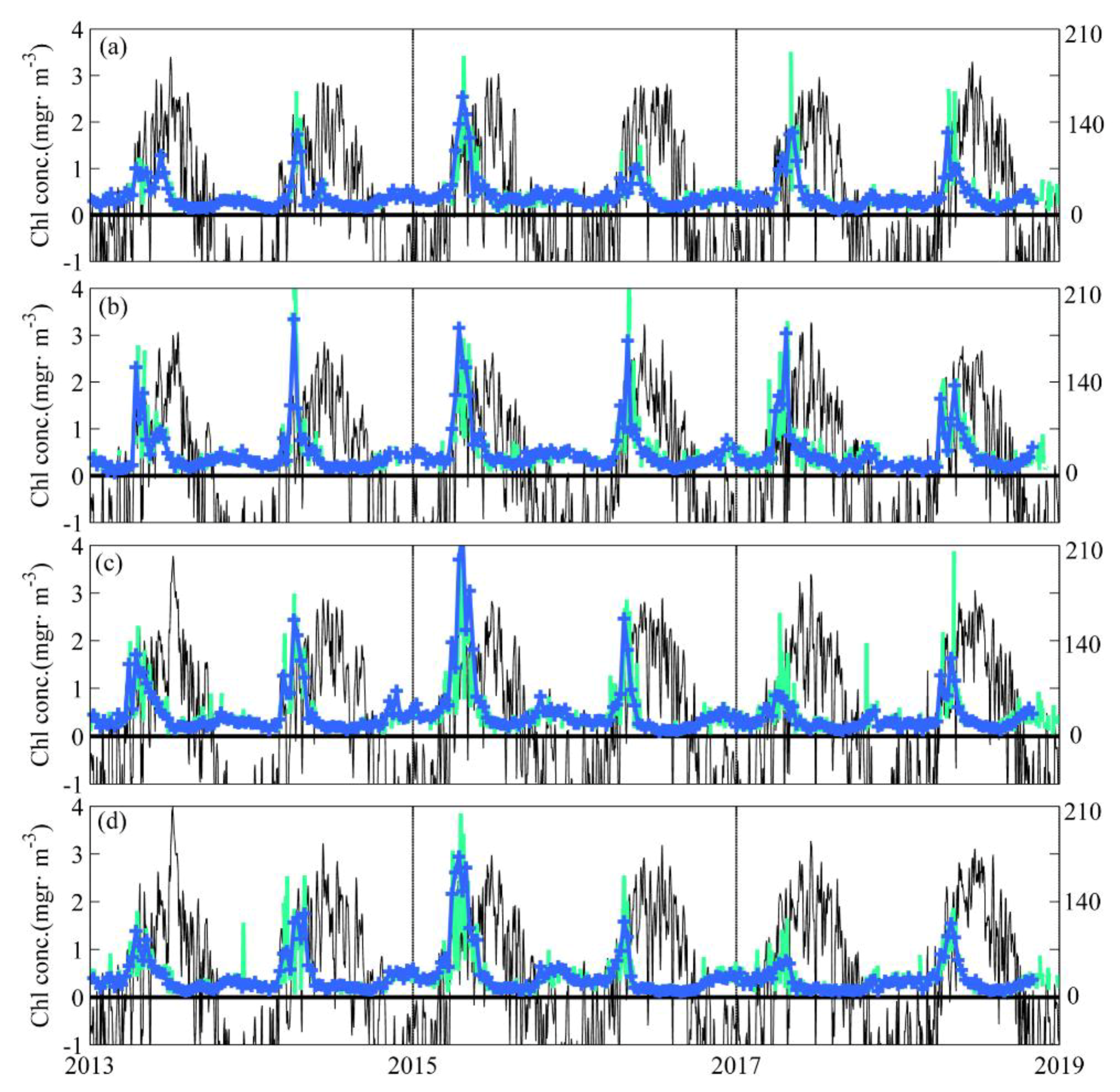
3.2. DCM Development: Change in Chlorophyll and Hydrographic Vertical Structure

Hydrological and chlorophyll vertical structure data confirm the previous conclusions surrounding the transition from the near-surface phytoplankton bloom towards a DCM. Climatologically, the onset of the spring bloom coincides with the moment at which Q₀ climatological seasonal cycle passes from negative to positive values (13th March; vertical red line in Figure 7a). In the water column, after the MLD reaches its maximum depth, a new, very shallow MLD begins to develop and the depth of chlorophyll (fluorescence) maximum during this time of the year is at its minimum (Figure 7b), exhibiting the highest annual values (the chlorophyll concentration at the depth of its maximum is the highest; Figure 4c,d). As typical at that time of the year, Q₀ is not permanently positive and oscillates between positive/negative values (stabilizing/destabilizing) and MLD alternates between very shallow and deep values (the stratification is still incipient and convective mixing can easily progress to the depths of the previous winter MLD) (Figure 7b; see additionally Figure 3 in [14]). Each deep mixing event entrains new nutrients into the mixed layer. Associated with stabilizing buoyancy moments (Q₀ > 0), in the new, very shallow MLD loaded with nutrients, phytoplankton burst occurs and the maximum chlorophyll concentration (proxy of phytoplankton biomass) is located above the MLD (Figure 4c,d and Figure 7b). Thus, phytoplankton growth responds to stabilizing/destabilizing buoyancy events (positive/negative Q₀), resulting in near-surface chlorophyll peaks observable from a satellite (Figure 5a and Figure 6) because they occur very close to the surface (Chl maximum is present from January to April within the layer that satellite ocean color observations integrates; Figure 4a–d). Overall, one can conclude that the initial cessation of convective mixing marks the onset of the spring bloom and its definitive shutdown determines its end. In between these two moments, when the alternation of convective mixing events (Q₀ < 0) entraining new nutrients in the mixed layer and stabilizing buoyancy moments (Q₀ > 0) allowing stratification to be established at the ocean surface enables phytoplankton growth in the near-surface layer, the spring bloom occurs.

While convective mixing events driven by negative Q₀ are able to reach the base of the MLD and inject new nutrients into the mixed layer, phytoplankton grows in this layer and the depth of the chlorophyll maximum is located above the MLD (Figure 7b and Figure 4b,c). Once no more convective mixing events take place until the following autumn–winter, no more new nutrients are entrained into the mixed layer. Then, phytoplankton growth occurs where there are still available nutrients: at the nutricline in the transition between the seasonal and permanent pycnocline (Figure 4f–i). Consequently, the depth where phytoplankton grows, and so the chlorophyll maximum deepens and passes from being located above the MLD—in an actively mixed layer—to being located below it in a comparatively stable parcel of the water column founding it permanently associated to the Typical Stable Water Structure (TSWS) [7] (Figure 7b and Figure 4f–i). It is from that moment that the near surface phytoplankton bloom evolves irremediably towards a DCM.

Climatologically, the last negative Q₀ event of the year able to reach the base of the MLD marks this transition. Based on the Q₀ −2STD climatological seasonal cycle (light blue line in Figure 5a), the definitive cessation of convective mixing late in spring is estimated to occur on the 11th of May (vertical light blue line in Figure 5a). It could be argued that it is a somehow arbitrary definition. However, consistently, this coincides with the moment at which the climatological seasonal cycle of Q_strg above the MLD in the water column becomes positive (4th of May; results not shown). As the last convective mixing episode must be strong enough to remove the accumulated heat above the MLD from the beginning of the spring, Q_strg above the MLD should be zero at that moment, increasing and becoming positive from then onwards.

3.3. Applicability of Our Results to other Ocean Regions and Further Remarks

Preliminary analyses using Bermuda Atlantic Time-series Study (BATS) oceanographic time-series data (see Figure A1 and Figure A2 in the Appendix A) seem to indicate that our conclusion is representative of other oceanic regions. In general, our approach is expected to be applicable to all those regions of the global ocean where air–sea heat exchange controls the seasonality of mixing and water column vertical structure (MLD and stratification). This is the case for all those regions of the open ocean of which their variation of the hydrographic (density) structure depends strongly on temperature, since the temporal evolution of the upper ocean temperature is dominated by its seasonal cycle, which is mostly driven by air–sea heat exchange (80%) [20]. In particular, it will be applicable to all those regions where there is a marked seasonal cycle in the net heat fluxes from the ocean to the atmosphere that determines a marked seasonal cycle of mixing in the upper layers where phytoplankton grows. These regions coincide with those denominated as temperate regions in biological studies. Ultimately, in these temperate regions, the seasonal cycle of the net heat flux from the ocean to the atmosphere and of the upper layer temperature are clearly related to varying solar heating (Q_sw). Alternatively, in tropical areas, in the absence of similar variations in solar inputs, the upper layer temperature and consequently the heat exchange with the atmosphere can vary seasonally due to subsurface cooling via mixing in tropical instability waves [26,27]. In this case, subsequent variations in the chlorophyll content of the water column and its vertical distribution (e.g., near-surface chlorophyll vs. DCM) will be determined by these mixing processes induced by tropical instability waves.

Apart from that, limitations to the applicability of our approach are expected especially if the study area moves from the ocean open to coastal zones. In ocean regions where upper ocean salinity dominates the density structure, and therefore the water column vertical structure, it is expected that air–sea heat exchange does not determine the onset of the spring bloom or its end and transition towards a DCM. In contrast to temperature, advection accounts for more than 70% of the budget terms for upper ocean salinity balance [20]. Thus, in regions where fresh water fluxes are significant, as in areas close to the coast, and affected by river discharges or melting glaciers, other processes may control the onset and duration of phytoplankton bloom. In the Labrador Sea, for example, offshore advection of Greenland meltwater flux, eddy activity, and their effects in haline stratification seems to be responsible for the early bloom in the northern Labrador Sea [28,29]. On the other hand, in the central basin of the Labrador Sea, the initiation of the surface spring bloom coincides closely with the timing of the first cooling-to-heating shift in air–sea heat fluxes [28,29] as in the study site used in this manuscript. SATS location, although apparently close to the coast, is not affected by the arrival of low salinity waters derived from river runoff until summer months when both the phytoplankton bloom and its transition towards a DCM have already occurred [20]. On this distinction between open ocean and coastal regimes, it must also be highlighted that, focused in the open ocean, our explanation of the end of the spring bloom and its transition towards a DCM is considered in a one-dimensional framework as in many other works [7]. At the transition between the continental shelf and the open ocean, other studies have pointed to allochthonous origins of DCMs through subduction of water masses along isopycnal surfaces ([30] and references therein).

Finally, we would like to emphasize that our findings regarding the drivers of the end of the spring phytoplankton bloom and its irreversible evolution towards a DCM do not contradict previous findings about the mechanisms that allow the development and maintenance of DCMs in relatively low mixed environments (e.g., subsurface production maxima caused by colimitation of photosynthesis by light and nutrients; photoacclimation processes; vertical migration, etc.) [7,31,32]. The occurrence of a DCM requires waters that remain stable long enough for its development (where phytoplankton grows), however different mechanisms can operate in the resulting Typical Stable Water Structure (TSWS) for its appearance and maintenance (how phytoplankton grows). Thus, our results just explain the relation between the definitive cessation of convective mixing and the end of the near-surface phytoplankton bloom -where phytoplankton grows in an actively mixed layer- and its transition towards a DCM -where phytoplankton grows in a comparatively stable parcel of the water column-.

4. Conclusions

The seasonal cycle of the net heat fluxes from the ocean to the atmosphere drives the seasonal cycle of mixing in the upper layers of the oceans where phytoplankton grows. It explains the finding that the onset of the spring bloom can be identified with the initial cessation of convective mixing when air–sea heat fluxes become positive (heat gain by the ocean surface), allowing incipient stratification to be established at the ocean surface along with phytoplankton growth [2,3]. Similarly, the definitive cessation of convective mixing (occurrence of the last heat loss event able to reach the base of the MLD) at the end of the spring that determines the last nutrient entrainment into the mixed layer marks the end of the near-surface bloom and its transition towards a DCM. From then onwards, phytoplankton grows below the MLD in a stable parcel of the water column evolving irreversibly towards a DCM.

Identified in this way, the spring bloom duration and the start of the transition towards a DCM can be systematically and objectively determined. At the study area, climatologically, this transition occurs on the 11th of May. Taking into account that climatologically the onset of the spring bloom occurs on the 13th of March, on average the spring bloom lasts 59 days. However, these dates can significantly vary from year to year (~± 20 days), making the maximum duration of the bloom able to double the minimum. Due to the importance of biomass accumulation associated with both the near-surface phytoplankton blooms and DCM for population dynamics of higher trophic levels and global biogeochemical cycles, precise knowledge about the timing when the near-surface bloom ends definitively and evolves irreversibly towards a DCM will provide sensitive indexes of climate and ecosystem variability.

Further investigation is needed to provide support that the definitive cessation of convective mixing and the end of the near-surface phytoplankton bloom and the transition towards a DCM is the likely mechanism operating in other oceanic regions, however preliminary analyses seem to indicate that our conclusion may be representative of mid-latitudes and subpolar regions of the global ocean.

References

1. Sverdrup, H. On conditions for the vernal blooming of phytoplankton. ICES J. Mar. Sci. 1953, 18, 287–295. [Google Scholar] [CrossRef]
2. Somavilla, R. Effects of Ocean-Atmosphere Interaction in the Upper Layers of the Bay of Biscay. Ph.D. Thesis, University of Cádiz, Cádiz, Spain, 2010. Available online: https://dialnet.unirioja.es/servlet/tesis?codigo=51752 (accessed on 10 July 2010).
3. Taylor, J.R.; Ferrari, R. Shutdown of turbulent convection as a new criterion for the onset of spring phytoplankton blooms. Limnol. Oceanogr. 2011, 56, 2293–2307. [Google Scholar] [CrossRef] [Green Version]
4. Behrenfeld, M.J. Abandoning Sverdrup’s Critical Depth Hypothesis on phytoplankton blooms. Ecology 2010, 91, 977–989. [Google Scholar] [CrossRef] [PubMed]
5. Latasa, M.; Cabello, A.; Morán, X.; Massana, R.; Scharek, R. Distribution of phytoplankton groups within the deep chlorophyll maximum. Limnol. Oceanogr. 2017, 2, 665–685. [Google Scholar] [CrossRef]
6. Herbland, A.; Voituriez, B. Hydrological structure analysis for estimating the primary production in the tropical Atlantic Ocean. J. Mar. Res. 1979, 37, 87–101. [Google Scholar]
7. Cullen, J.J. Subsurface chlorophyll maximum layers: Enduring enigma or mystery solved? Annu. Rev. Mar. Sci. 2015, 7, 207–239. [Google Scholar] [CrossRef] [PubMed]
8. Waniek, J.; Holliday, N. Large-scale physical controls on phytoplankton growth in the Irminger Sea, Part ii: Model study of the physical and meteorological preconditioning. J. Mar. Syst. 2006, 59, 219–237. [Google Scholar] [CrossRef]
9. Behrenfeld, M.; Boss, E. Resurrecting the Ecological Underpinnings of Ocean Plankton Blooms. Mar. Sci. 2014, 6, 167–194. [Google Scholar] [CrossRef] [PubMed]
10. González-Pola, C.; Lavín, A.; Vargas-Yánez, M. Intense warming and salinity modification of intermediate water masses in the southeastern corner of the Bay of Biscay for the period 1992–2003. J. Geophys. Res. Oceans 2005, 110, 1–14. [Google Scholar] [CrossRef]
11. Somavilla, R.; González-Pola, C.; Rodriguez, C.; Josey, S.A.; Sánchez, R.F.; Lavín, A. Large changes in the hydrographic structure of the Bay of Biscay after the extreme mixing of winter 2005. J. Geophys. Res. 2009, c01001. [Google Scholar] [CrossRef]
12. Somavilla, R.; González-Pola, C.; Villarreal, M.; Lavín, A. Mixed layer depth variability in the southern Bay of Biscay. Deepening of winter MLDs concurrent to generalized upper water warming trends? Ocean Dyn. 2011, 61, 1215–1235. [Google Scholar] [CrossRef]
13. Somavilla, R.; González-Pola, C.; Schauer, U.; Budéus, G. Mid-2000s North Atlantic shift. Heat budget and circulation changes. Geophys. Res. Lett. 2016, 43, 2059–2068. [Google Scholar] [CrossRef] [PubMed]
14. Somavilla, R.; González-Pola, C.; Fernández-Diaz, J. The warmer the ocean surface, the shallower the mixed layer. How much of this is true? J. Geophys. Res. Oceans 2017, 122, 7698–7716. [Google Scholar] [CrossRef] [PubMed] [Green Version]
15. Kalnay, E.; Kanamitsu, M.; Kistler, R.; Collins, W.; Deaven, D.; Gandin, L.; Iredell, M.; Saha, S.; White, G.; Woollen, J.; et al. The NCEP/NCAR 40-year reanalysis project. Bull. Am. Meteorol. Soc. 1996, 77, 437–471. [Google Scholar] [CrossRef]
16. Somavilla, R.; Lavín, A.; Rodriguez, C.; Cano, D. AGL buoy. A high frequency view of processes at the air-sea interface. In Proceedings of the IEEE Oceans 2011-Europe, Santander, Spain, 6–9 June 2011. [Google Scholar] [CrossRef]
17. Fairall, C.; Bradley, E.; Rogers, D.; Edson, J.; Young, G. Bulk parameterization of air-sea fluxes for tropical ocean global atmosphere coupled ocean atmosphere response experiment. J. Geophys. Res. 1996, 101, 3747–3764. [Google Scholar] [CrossRef]
18. Yu, L.; Jin, X.; Weller, R.A. Multidecade Global Flux Datasets from the Objectively Analyzed Air-Sea Fluxes (OAFlux) Project: Latent and Sensible Heat Fluxes, Ocean Evaporation, and Related Surface Meteorological Variables; OAFlux Project Technical Report: Woods Hole, MA, USA, 2008; OA-2008-01, 64. [Google Scholar]
19. Cronin, M.; McPhaden, M. The upper ocean heat balance in the western equatorial pacific warm pool during September–December 1992. J. Geophys. Res. 1997, 102, 8533–8553. [Google Scholar] [CrossRef]
20. Somavilla, R.; González-Pola, C.; Lavín, A.; Rodriguez, C. T and S variability in the south-eastern corner of the Bay of Biscay (NE Atlantic). J. Mar. Syst. 2013, 109–110 (Supplement), S105–S120. [Google Scholar] [CrossRef]
21. González-Pola, C.; Fernández-Diaz, J.M.; Lavín, A. Vertical structure of the upper ocean from profiles fitted to physically consistent functional forms. Deep Sea Res. Part I 2007, 54, 1985–2004. [Google Scholar] [CrossRef]
22. Sauzède, R.; Claustre, H.; Jamet, C.; Uitz, J.; Ras, J.; Mignot, A.; D’Ortenzio, F. Retrieving the vertical distribution of chlorophyll a concentration and phytoplankton community composition from in situ fluorescence profiles: A method based on a neural network with potential for global-scale applications. J. Geophys. Res. Oceans 2015, 120. [Google Scholar] [CrossRef]
23. Kantha, L.H.; Clayson, C.A. Small Scale Processes in Geophysical Fluid Flows; International Geophys; Academic Press: Cambridge, MA, USA, 2000; Volume 67. [Google Scholar]
24. Alexander, M.A.; Scott, J.D.; Deser, C. Processes that influence sea surface temperature and ocean mixed layer depth variability in a coupled model. J. Geophys. Res. 2000, 105, 16823–16842. [Google Scholar] [CrossRef] [Green Version]
25. Cronin, M.F.; Sprintall, J. Wind and buoyancy-forced upper ocean. In Encyclopedia of Ocean Sciences; Steele, J.H., Turekian, K.K., Thorpe, S.A., Eds.; Academic Press Ltd.: Cambridge, MA, USA, 2011; pp. 3219–3227. [Google Scholar]
26. Moum, J.; Lien, R.-C.; Perlin, A.; Nash, J.D.; Gregg, M.C.; Wiles, P.J. Sea surface cooling at the Equator by subsurface mixing in tropical instability waves. Nat. Geosci. 2009, 2, 761. [Google Scholar] [CrossRef]
27. Moum, J.N.; Perlin, A.; Nash, J.D.; McPhaden, M.J. Seasonal sea surface cooling in the equatorial Pacific cold tongue controlled by ocean mixing. Nature 2013, 500, 64. [Google Scholar] [CrossRef]
28. Frajka-Williams, E.; Rhines, P. Physical controls and interannual variability of the Labrador Sea spring phytoplankton bloom in distinct regions. Deep Sea Res. Part I Oceanogr. Res. Pap. 2010, 57, 541–552. [Google Scholar] [CrossRef] [Green Version]
29. Marchese, C.; Guardia, L.; Myers, P.; Bélanger, S. Regional differences and inter-annual variability in the timing of surface phytoplankton blooms in the Labrador Sea. Ecol. Indic. 2019, 96, 81–90. [Google Scholar] [CrossRef]
30. Erickson, Z.; Thompson, A.; Cassar, N.; Sprintall, J.; Mazloff, M. An advective mechanism for deep chlorophyll maxima formation in southern Drake Passage. Geophys. Res. Lett. 2016, 43, 10846–10855. [Google Scholar] [CrossRef]
31. Cullen, J.J. The deep chlorophyll maximum: Comparing vertical profiles of chlorophyll a. Can. J. Fish. Aquat. Sci. 1982, 39, 791–803. [Google Scholar] [CrossRef]
32. Mitchell, B.G.; Brody, E.A.; Holm-Hansen, O.; McClain, C.; Bishop, J. Light limitation of phytoplankton biomass and macronutrient utilization in the Southern Ocean. Limnol. Oceanogr. 1991, 36, 1662–1677. [Google Scholar] [CrossRef] [Green Version]
Figure 1. Upper: Map of the North Atlantic Ocean showing the location of the mid-latitudes of the Eastern North Atlantic (ml-ENA, red box in the map). Lower: Zoom to ml-ENA where Santander Atlantic-Time-Series (SATS) oceanographic station is located (red dot in the map). The location of the remaining stations of the Santander standard section are also shown (orange dots).
Geosciences 09 00178 g001
Figure 2. Air-sea heat fluxes registered by the oceanic-meteorological buoy (AGL) buoy since its deployment in June 2007. (a) Short (solar, Qsw) and long-wave (Qlw) radiative heat flux components (black and blue lines, respectively) obtained from NCEP/NCAR Reanalysis. (b) Latent (QE) and Sensible (QH) turbulent heat flux components (black and blue lines, respectively) estimated from AGL buoy data. Qlw, QH, and QE are expressed as heat loss by the ocean surface (heat loss implies negative values and are represented as −Qlw, −QE, and −QH for clarity). (c) Net heat flux (Q0) as a result of the sum of radiative and turbulent heat flux components. Red lines in (ac) show the climatological seasonal cycles of Qsw, QE, and Q0 through Fourier decomposition.
Geosciences 09 00178 g002
Figure 3. Comparison of latent (QE) and Sensible (QH) turbulent heat flux components estimated from AGL buoy data and obtained from NCEP/NCAR (orange dots) and OAFLUX (blue dots) reanalysis data sets.
Geosciences 09 00178 g003
Figure 4. Fluorescence profiles obtained at SATS oceanographic station from January to December. All profiles taken from January 1998 (beginning of the use of CTD equipped with fluorescence sensor) to December 2018 are included and plotted in the corresponding month (grey thin profiles). Randomly, for each month, one profile is highlighted (black profile), also showing its corresponding 5 m low-pass filter profile (thick grey) and the depth at which fluorescence shows its maximum value on this filtered profile (green line). For these randomly selected fluorescence profiles, their corresponding density profiles are also shown (red line) as well as the estimated MLD (purple horizontal line). The x-axis only shows the fluorescence scale (density profiles were re-scaled to be shown on this scale since the interest is the upper ocean vertical structure, which is observable just from density profiles topology). Note that the x-axis is not the same for the different subplots. The pink shadow area in each subplot shows the depth range integrated by satellite measurements (1/5 of the euphotic zone calculated as the depth at which 1% of the PAR at the surface penetrates [22]).
Geosciences 09 00178 g004
Figure 5. (a) Surface chlorophyll concentration derived from AGL buoy hourly fluorescence measurements at 3 m depth (green line) and from weekly satellite-derived Chlorophyll a concentration from GlobColour project (blue cross line). (b) Net heat flux (Q0) (black line) from the ocean to the atmosphere (negative values imply a heat loss by the ocean). Gaps in Q0 time-series estimated from AGL buoy data are filled with that obtained from NCEP/NCAR reanalysis (grey line). Blue dots show the accumulated heat storage above the mixed layer depth (MLD) (Qstrg) estimated from hydrographic profiles from SATS oceanographic station. It is shown as −Qstrg to facilitate the identification of net heat loss events sufficiently negative to remove Qstrg above the MLD (Q0 < −Qstrg). The red curve shows the accumulated net heat flux. The grey shadow areas mark the time period each year between: (1) the initial moment in which the net heat flux becomes “effectively” positive (Q0 (black line) passes from negative to positive values and the accumulated Q0 starts to increase) and (2) the definitive cessation of convective mixing when the last net heat loss event sufficiently negative to reach the base of the MLD occurs (sufficiently negative to remove Qstrg above the MLD). In 2018, a first small peak in near-surface Chl coinciding with a short-live Q0 > 0 event is highlighted in light grey. The largest peak occurs when Q0 becomes “effectively” positive.
Geosciences 09 00178 g005
Figure 6. Surface chlorophyll concentration from daily (green line) and weekly (blue cross line) satellite-derived Chlorophyll a concentration from GlobColour project and net heat flux (Q0) (black line) from the ocean to the atmosphere (negative values imply a heat loss by the ocean) at different locations in the mid-latitudes of the Eastern North Atlantic. (a) at the grid centered at 44.76° N, 15° W from NCEP/NCAR reanalysis data. Chlorophyll time-series are obtained as the average daily and weekly time-series within this grid 44.76°N ± 1.9 /2° N and 15° W ± 1.9/2° E (NCEP/NCAR spatial resolution is 1.9° × 1.9°). (bd) idem at the grids at 46.67° N, 5.62° W; 44.76° N, 9.38° W; and 42.86° N, 11.25° W. Chlorophyll concentration scale is shown in the left y-axis in mgr·m−3 and Q0 in the right y-axis in W·m−2.
Geosciences 09 00178 g006
Figure 7. (a) Net heat flux (Q0) from the ocean to the atmosphere. All mean daily values registered since 2007 by the AGL buoy are shown (black dots). The climatological seasonal cycle obtained from these values is shown by the red line. The blue line shows the Q0 −2STD climatological cycle. (b) Depths of the Deep Chlorophyll Maximum (DCM) (green dots) and MLD (black dots) estimated on chlorophyll and density profiles registered at SATS oceanographic station. The vertical red line in (a) and (b) marks the date in which Q0 climatological seasonal cycle becomes positive. Idem for the light blue line and the Q0 −2STD climatological seasonal cycle. The dark blue line in (a) marks the date at which Q0 climatological seasonal becomes negative in late summer.
Geosciences 09 00178 g007