Article

Transient Thermal Effects in Sedimentary Basins with Normal Faults and Magmatic Sill Intrusions—A Sensitivity Study

by
Magnhild Sydnes
1,2,*,
Willy Fjeldskaar
1,
Ivar Grunnaleite
1,
Ingrid Fjeldskaar Løtveit
1 and
Rolf Mjelde
2
1
Tectonor AS, P.O. Box 8034, NO-4068 Stavanger, Norway
2
Department of Earth Science, University of Bergen, Box 7803, 5020 Bergen, Norway
*
Author to whom correspondence should be addressed.
Geosciences 2019, 9(4), 160; https://doi.org/10.3390/geosciences9040160
Submission received: 13 March 2019 / Revised: 29 March 2019 / Accepted: 2 April 2019 / Published: 5 April 2019

Abstract

:
Magmatic intrusions affect the basin temperature in their vicinity. Faulting and physical properties of the basin may influence the magnitudes of their thermal effects and the potential source rock maturation. We present results from a sensitivity study of the most important factors affecting the thermal history in structurally complex sedimentary basins with magmatic sill intrusions. These factors are related to faulting, physical properties, and restoration methods: (1) fault displacement, (2) time span of faulting and deposition, (3) fault angle, (4) thermal conductivity and specific heat capacity, (5) basal heat flow and (6) restoration method. All modeling is performed on the same constructed clastic sedimentary profile containing one normal listric fault with one faulting event. Sills are modeled to intrude into either side of the fault zone with a temperature of 1000 °C. The results show that transient thermal effects may last up to several million years after fault slip. Thermal differences up to 40 °C could occur for sills intruding at time of fault slip, to sills intruding 10 million years later. We have shown that omitting the transient thermal effects of structural development in basins with magmatic intrusions may lead to over- or underestimation of the thermal effects of magmatic intrusions and ultimately the estimated maturation.

1. Introduction

Hydrocarbon discoveries associated with magmatic intrusions are common in many sedimentary basins throughout the world [1,2,3], and these intrusions may potentially affect all parts of the petroleum system [4]. The impact of magmatic intrusions has been studied in several basins worldwide, e.g., Vøring Basin, Norway (e.g., [5,6,7]), Karoo Basin, South Africa (e.g., [8,9,10]), Gunnedah Basin, Australia [11], Neuquén Basin, Argentina (e.g., [12,13]), Bohai Bay Basin, China (e.g., [14,15]). All these studies conclude that magmatic intrusions significantly influence the basin thermal history and thus the maturation of organic material in their vicinity.
Several studies have identified the pre-intrusion temperature of the host rock as an important variable for the ultimate thermal and maturation levels of sedimentary basins with magmatic intrusions [8,10,13,16,17,18]. However, this variable is one of the most difficult parameters to constrain, as the traces of pre-intrusion temperature and maturation are erased instantly in the thermal aureole of magmatic intrusions when magmatic emplacement occurs [19] and the basin has been subject to later geological development. As magmatic intrusions often are emplaced into structurally complex sedimentary basins, it is crucial to understand how the basin’s structural evolution affects the temperature development. With such knowledge it should be possible to discern temperature effects of the structural development from temperature effects of magmatic intrusions. This is important as the pre-intrusion temperatures have implications for the magnitude of the thermal effect of sills, i.e., size and temperatures of the thermal aureole, which eventually will have implications for the estimated maturation of the basin.
Magmatic intrusions and their effect on temperature and maturation in the surrounding host rocks have been subject of several studies (e.g., [8,13,19,20,21,22,23,24]). Only a few studies model sills intruding into structurally complex basins under development, while taking the temporary host-rock temperature and maturation into consideration (e.g., [7,25]). Structurally complex basins are characterized by numerous faults, changing lithologies with different physical properties and area specific heat flow. To estimate the basin’s thermal development as a function of time, the geohistory of the basin must first be established by reconstruction. In standard basin modeling, the impact of the structural development on the temperature history is seldom taken into account and this may give incorrect thermal and maturation predictions [26].
Several studies exist on temperature modeling in fault zones, but many of these focus on the effects related to uplift and erosion observed in the footwall part of the fault zone and not on the thermal transients in the hanging wall section (e.g., [27,28,29,30,31,32,33,34]). To our knowledge no studies includes magmatism in a fault setting. In our study the main focus is on the transient thermal effects of normal faults with syn- and post-rift deposits, and the influence such structural development has on the thermal effects of sills. Possible transient thermal effects due to erosion have not been pursued in this study.
The calculated pre-intrusion temperatures are dependent on the representation of the basin’s structural development [13,25,26]. The purpose of this study is to quantify the thermal effects of the most important factors affecting the thermal history in structurally complex sedimentary basins with magmatic sill intrusions. We do this by running a series of simple models. A more realistic model would require higher structural resolution with variation of lithological and geometrical properties in space and time. However, many simultaneously varying factors affecting the thermal evolution would obscure the magnitude and impact of the individual factors. We therefore first study the thermal effects on structural complex basin on a simple, synthetic profile followed by analysis of the subsequent sensitivity sets: (1) fault displacement, (2) time span of faulting and deposition, (3) fault angle, (4) thermal conductivity and specific heat capacity, (5) basal heat flow and (6) restoration method. The overall goal is to test the sensitivity of faulting, physical properties of the lithologies and choice of fault restoration method on the thermal effect of magmatic intrusions in complex sedimentary basins. We aim for some general conclusions that are applicable to sedimentary basins with normal faults and magmatic sill intrusions.

2. Methods

Our study investigates the relative effect faulting, different physical properties and choice of restoration method have on the resulting thermal and maturation history in structurally complex sedimentary basins intruded by sills. A simple, synthetic profile containing one listric fault and a number of horizons, including syn- and post-rift deposits, is used as the basis for this study (Figure 1). Throughout the simulations, one parameter is changed at a time which allows for evaluating the impact each parameter has on the modeling results. Table 1 shows the different modeling sets, the tested parameter values and default values of non-changing parameters. Shale and sandstone are the applied lithologies as these are common in sedimentary basins worldwide.

2.1. Thermal and Maturation Modeling

The geological, structural, thermal, and maturation history of the studied synthetic profile is performed with BMT (Basin Modelling Toolbox, Tectonor AS), a high-resolution 2D basin modeling software [26,35,36]. All thermal and maturation modeling simulations starts with present day geometry, where every horizon is given a specific age and all polygons are assigned a lithology with related porosity/depth trend, thermal conductivity and specific heat capacity (Table 2, upper part).
The first modeling step is a backstripping process, where one horizon at a time is removed, faults are restored and underlying deposits are decompacted. This process is repeated all the way down to top basement and in this way the section’s geohistory is built. All elements that characterize the basin, such as faults, horizons, and lithologies, are parts of the geohistory process, and must be carefully defined. For the geohistory reconstruction a special type of grid was developed in BMT [26]. The grids are vertical line segments that are connected to the base of a polygon. A grid is always created at each digitized point in the present-day polygon. Additional grid columns are added to the section automatically. The number of inserted grid points can be controlled by the user (the default is 70). The foundation for thermal and maturation modeling is established during the geohistory process, and it is therefore important that the geological reconstruction of the basin is accurate.
The next step in the modeling process is the thermal development of the basin. BMT utilizes finite difference calculations by conduction with a rectangular finite difference grid of varying sizes (cf., [7,26]). For every reconstructed timestep in the geohistory, BMT builds a new high-resolution thermal modeling grid. Where needed, grid lines are automatically inserted so that the geometry is accurately represented. Around small features, like sills, the grid size is especially fine to ensure realistic calculations. The finite difference grid in this study consists of minimum 400 × 400 cells of varying sizes with an average size of 80 m × 30 m (width and height). The spatial variation in rock properties and possible differences from one timestep to the next are adjusted for so that appropriate finite difference calculations are maintained.
The finite difference calculation by conduction is controlled by the temperatures from the previous timestep, thermal conductivity (vertical and horizontal) and specific heat capacity of the basin’s lithology/lithologies (see Appendix A for details on the numerical temperature model from Fjeldskaar et al. [7]). Temperature-dependent thermal conductivity is used, which commonly leads to reduction of the conductivity with increasing temperature. However, compared to conduction variations derived from differences in porosity and lithology, the temperature dependent variations are considered to be modest [35]. The lower boundary condition of the temperature calculations is the basal heat flow from the mantle, and the upper boundary condition is the paleo-surface temperature. The surface temperature is kept constant at 7 °C, and the heat flow is constant over the profile. Fjeldskaar et al. [7] tested BMT’s numerical model versus an analytical model on the temperature effect of sill emplacement, and documented good performance for high-resolution modeling, both spatially and temporally.
Maturity modeling is completed in BMT and all calculations in this study assume kerogen type II, the most common in marine shales [39]. Classical first-order kinetics for the decomposition reactions is the basis for the maturation model in BMT (see [7,26]). In this study the whole basin is set as source rock in order to study the potential maturation effect of magmatic sill intrusions. However, for a case study, only the potential source rock would be defined as such a sequence.

2.2. Restoration of Faults

Several algorithms exist for restoring the structural evolution of basins. The different algorithms result in different basin and fault geometries, which again impact the calculated thermal history. Commonly, basin modeling simplifies the structural reconstruction of basins, e.g., by not reconstructing the faults through time, regardless the fact that hydrocarbons often accumulate in complex geological structures associated with faults [26]. According to Dula [40] reconstruction with simple inclined antithetic shear of 20° is one of the methods that best represents the observed fault shape, but all tested reconstruction methods in that study gave adequate results.
The present study utilizes vertical shear as a standard fault reconstruction method. However, different segments of simple shear, including inclined antithetic and synthetic shear are explored (Figure 2). Furthermore, we investigate how the different resulting geometries impact the thermal history. Because BMT restore faults solely by vertical shear, and the software Move (Petex Ltd.) does not have the ability to perform thermal and maturation modeling, both Move and BMT were used to model the structural development of the section. In the restoration process BMT and Move both use the backstripping process, which removes layers one by one and decompact the underlying sequences based on the given porosity-depth trend for the assigned lithology/lithologies. The porosity calculations are based on exponential functions (cf., [37]) and the same values are used in both softwares (Table 2). Move is a commercial software restoring geological cross sections by kinematic algorithms. Six algorithms are available for fault restoration, these are: simple shear, fault parallel flow, fault bend fold, fault propagation fold, trishear, and detachment fold. BMT is a non-commercial basin modeling software with the ability to perform fault restoration (by vertical simple shear) so that structural effects on temperature estimates are accounted for (cf., [26]).
In our study Move was used to restore the fault by antithetic and synthetic inclined shear. The tested angles for inclined shear are summarized in Table 1. The resulting reconstructions from Move are replicated in BMT by utilizing a “volume editing” function (cf., [26]). This method enables calculations of the thermal histories for the different restoration methods. All models have the same starting geometry. However, through restoration by different algorithms the paleo geometries will differ and so will the temperature histories.

2.3. Thermal Effects of Sills

On reflection seismic data, upper and lower boundaries of sills can be difficult to discern due to limited vertical resolution (cf., [42,43,44,45]). Many sills may therefore be left out in seismic interpretations due to sill thicknesses below the detection limit of the data (e.g., [44,45]). Sill thickness, both when sills intrude individually or as clusters, has a large impact on the temperature and maturation in sedimentary basins (e.g., [8,25]). The relative timing between sills emplaced as clusters is especially important if potential source rocks are located between sills [25]. Reported sill thicknesses from the literature vary from ~10 cm to >400 m (e.g., [44,46,47,48,49,50,51,52,53,54,55]). In our study a modest sill thickness of ~50 m has been chosen for the modeled sills and we assume the sills to intrude during one pulse with a magma temperature of 1000 °C. In BMT this is done by changing the lithology in sill polygon from shale to sill lithology, with related physical properties at time of intrusion. The sills have been modeled to intrude at various times relative to fault slip. This is done to study the interaction of two transient thermal effects simultaneously. As the largest thermal and maturation impact of sill intrusions are found at 3–5 km depths [25], the sills are modeled to intrude within this depth range. Commonly magmatic sills observed in the field and on seismic images (e.g., [7,52]) are layer concordant. Therefore, the sills in the study are modeled accordingly.
Latent crystallization heat introduces an extra source of heat when magma cools and starts to crystallize [56,57]. This extra heat source is not taken into account, as it is the relative differences between scenarios that are of interest in our study. Heat advection by fluids in relation to magmatic intrusions is common (e.g., [5,58,59,60,61]). However, convection is not accounted for in our modeling, as convection is considered insignificant in low permeability rocks (e.g., [7,8,13,25,62]) and is beyond the scope of this study.

3. Modeling Strategy and Results

A basin not subjected to tectonic deformation undergoes a slow rate of erosion or sedimentation and has a gradual temperature increase with burial depth. Such a basin is in steady state [63]. On the other hand, structurally active basins may undergo sudden erosion or high influx of sediments, e.g., due to increased accommodation space during faulting, leading to abrupt changes in the geothermal gradient. When magmatic intrusions are emplaced into such active basins, the temporary, local change in temperature is not solely an effect of the hot magma intruding the system, but also due to transient thermal effects caused by structural development. Figure 3 shows the studied synthetic profile assuming thermal steady state with input parameters as given in Table 2.
Emplacement of sills and significant structural development may occur within the same timeframe (e.g., [30,64,65]). Therefore, we want to investigate the combined transient thermal contributions from the structural development and magmatic intrusions. The results should be considered as trends, not absolute values, as the study aim to give some general conclusions. The models are considered to have arrived at steady state when the whole basin show transient temperatures <1 °C from the steady state temperatures. However, for some cases exact steady state conditions are obtained right after reaching this limit, for other cases several million years (Myr) are required before actual steady state is obtained.

3.1. Thermal Effect of Slip along a Single, Normal Fault

Normal faulting causes downward displacement of sediments and generally deposition of syn-rift sediments (ref., Figure 1) in the hanging wall section of the fault zone. These down faulted sediments in the hanging wall are initially colder than the sedimentary rocks at the same depth in the footwall part, which result in transient thermal effects mostly in the hanging wall part (Figure 4). The basin is thermally unstable and results in a temperature difference up to 40 °C from one side of the fault zone to the other at the time of fault slip (Figure 4). Post-rift sediments deposited over the whole basin leads to thermal transient effects also in the foot wall section. However, these temperature differences will vary depending on physical properties and geometry of the basin. In the event of extension and normal faulting, the footwall temperatures are hardly influenced at time of fault slip. At 1000 years after the fault movement the isotherms in the footwall show a small downward bend towards the fault zone, indicating a small thermal influence by the neighboring colder sediments in the hanging wall (Figure 4).
The main temperature effect of magmatic sills lasts only some thousand years (see e.g., [25]). In accordance with this, we have here assumed that the syn- and post-rift sediments (Figure 1) of the timestep with fault movement are deposited over a period of only some thousand years. Deposition of these sediments leads to thermal instability in the basin. Figure 5 shows the temperature difference between steady state and transient models for deposition of these sediments at 10,000 years (10 kyr) and 500 kyr after fault slip. This causes larger parts of the basin to have transient temperatures up to 20 °C lower than under steady state conditions even up to 500 kyr after fault slip (Figure 5). Around 10 Myr is required for the basin to reach steady state temperatures.

3.1.1. Fault Displacement

The original model has a fault displacement of 1200 m with syn-rift deposits of the same thickness and about 600 m of post-rift deposits, taking place over one timestep (Figure1). These post-rift deposits are kept unchanged in all tested scenarios. Additional four fault displacement models were tested; 500 m, 1000 m, 2000 m, and 3000 m (Table 1). As expected, temperature differences across the fault zone increases with the fault displacement. With 3000 m fault slip there is a temperature difference of more than 50 °C across the fault zone immediately after fault slip (Figure 6a). In the footwall part, the isotherms make a gentle downward bend towards the fault zone. As time passes, a gradual heating of the sediments in the hanging wall section occurs and the bend of the isotherms from the footwall side ties with those of the hanging wall (~10 kyr after faulting) creating continuous isotherms (Figure 6b,c). There is also a slight temperature change in the footwall part due to the deposition of cold post-rift sediments over that area.
With increasing fault slip but within the same timeframe, the volume of deposited sediments and time needed for basin to regain steady state increases. For the modeled basin with 500 m of fault slip, large parts of the basin differ ~20 °C from the steady state basin 10 kyr after displacement (Figure 7a). Around 9 Myr later the basin obtains steady state. When fault displacement is 3000 m, large parts of the hanging wall section differ more than 50 °C from the steady state basin at 10 kyr after fault slip (Figure 7b). Steady state is achieved approximately 11 Myr after fault slip. As expected a basin with larger fault slip and higher influx of sediments requires more time to regain steady state, compared to a basin with smaller fault slip and less sediment deposits.

3.1.2. Time Span of Faulting and Deposition

So far the modeling assumes the fault slip to be almost instantaneous (taking place over 10 kyr). The next set of models explores four different time spans of faulting and deposition of the same amount of sediments: 1, 5, 10, and 20 Myr. The results show that slower faulting and deposition rates, as expected, keep the basin closer to a steady-state condition compared to high rates (Figure 8a,b). Adding 10 Myr to the faulting and deposition time results in a basin with transient temperatures much closer to those of steady state throughout the whole period. For a faulting and deposition rate over 20 Myr, the basin is never in a state of thermal instability. The resulting trend show that basins with the same amount of sediment input and faulting and deposition time up to 10 Myr regains steady state approximately 10 Myr after faulting initiated (Figure 8c). This means that from time of faulting and deposition to the process is finalized, more time is required for a basin with rapid fault slip and deposition to regain steady state compared to a basin with slow fault slip and deposition. It emphasizes how crucial the time relation is for faulting and deposition and basin’s thermal development after fault slip.

3.1.3. Fault Angle

The previous results show that the largest thermal differences between steady state and transient temperatures are found in the hanging wall part of the basin. For all the tested fault angles the results are broadly similar, but the temperature effect will change with the fault angle. As the fault angle is changed, so is the affected area of the hanging wall. With a steeper fault angle a smaller part of the basin experiences the largest thermal instabilities (Figure 9a). The opposite is the case for lower fault angles, a larger part of the basin will then experience higher thermal instabilities before the basin regain steady state (Figure 9b). Five different fault angles have been tested (Figure 9a,b). All scenarios show temperature differences up to 45 °C between transient and steady state models. Around 10 Myr after fault slip all scenarios regain steady state temperatures.

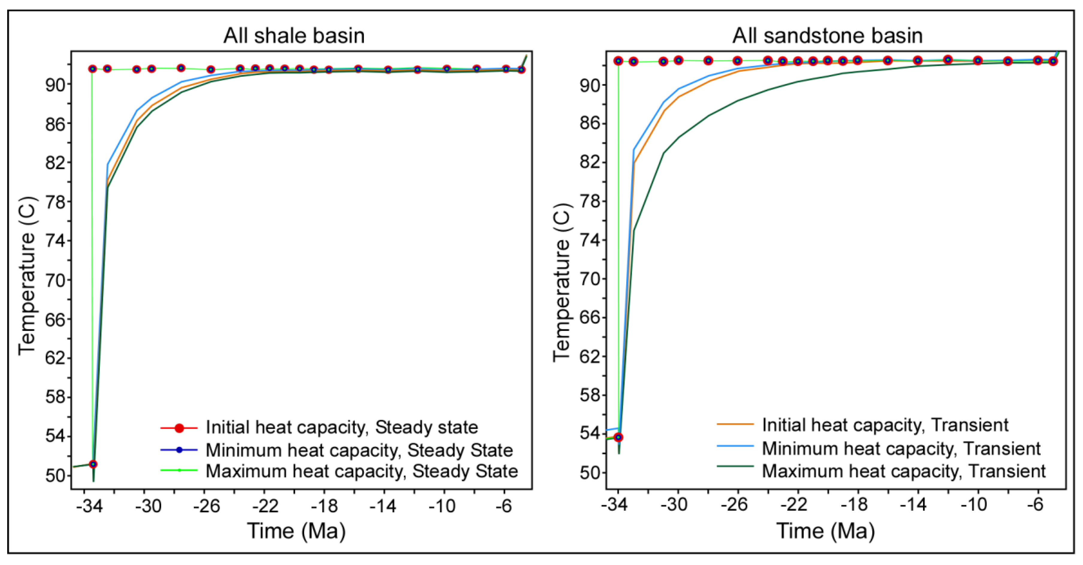
3.1.4. Thermal Conductivity and Specific Heat Capacity

The thermal conductivity (W·m−1·K−1) of a lithology relates to the rock’s ability to transfer heat. Rocks with low thermal conductivity result in warm basins, while high thermal conductivity rocks give colder basins. A lithology’s specific heat capacity (J·kg−1·K−1) is the physical property crucial for the time frame needed to transfer heat through the stratum and thus for the time needed for basins to regain steady state after sediment deposition or erosion. So far the section has been modeled as all shale with properties as listed in Table 2. Commonly, basins consist of altering layers of different lithology types, often shale and sandstone. Therefore, the following four scenarios have been compared: all shale, all sandstone, all shale with one sandstone layer, and all sandstone with one shale layer.
Thermal conductivities and specific heat capacities of shale and sandstone show a large variation (e.g., values in Table 2). The default values are given in Table 2 and to illustrate the span of values within the same lithology segment, we refer to Čermác and Rybach [38]. Their minimum and maximum specific heat capacities and the average and maximum thermal conductivities of sandstone and shale are used in this study (Table 2). In order to determine the thermal conductivity values based on the rock’s porosity, the mixing law arithmetic mean model [66] has been used:
k = ɸ·kf + (1 − ɸ)ks,
where the thermal conductivity (k) is obtained on the basis of the rock porosity (ɸ) by combining the thermal conductivity of rock matrix (ks) with that of the pore fluid (kf).
Generally, sandstones have higher thermal conductivities than shales, resulting in colder basins where they are abundant. The results from the homogeneous basins, either all shale or sandstone, coincide with this, showing high temperatures in the basin when the thermal conductivity is low, and lower temperatures when the thermal conductivities are high. A comparison between two basins with the same fixed specific heat capacity, but with one basin modeled with average shale conductivity, to another basin modeled with default shale conductivity, shows up to 140 °C difference between the two models shortly after fault slip (Figure 10a). With fixed specific heat and changing conductivity the results show that the basin needs longer time to regain steady state in basins with low thermal conductivity values due to the higher temperatures obtained in these basins (Figure 10b). This applies for both scenarios with all shale and all sandstone of varying thermal conductivity. Steady state is regained from 3–22 Myr after fault slip and the quickest scenario to regain steady state is the sandstone basin with maximum thermal conductivity.
In the case where the thermal conductivity is fixed and the specific heat capacities are changed in the different modeling scenarios (Table 2, lower part), the steady state temperatures for all the scenarios are, as expected, the same (Figure 11). However, with increasing specific heat, the time needed for the basin to obtain steady state increases (Figure 11). This is especially visible in the point plot for sandstone basin in Figure 11, because of large difference in the published heat capacity values of sandstone, but the effect is also visible for the shale basin. For all tested scenarios steady state is obtained between 8–18 Myr after fault slip.
To accommodate the fact that basins commonly consists of different lithologies, the polygon with syn- and post-rift deposits have been changed in the following simulation (Figure 12a). The thermal conductivity is fixed with values as for the default shale or sandstone (Table 2). However, the specific heat capacity is changed using default, minimum, and maximum values for the sandstone and shale (Table 2). With the presence of a sandstone layer in an otherwise shale basin, the results show that the temperatures in the basin increases. For the opposite case, a layer of shale in an otherwise sandstone basin, the temperatures in the basin decreases (Figure 12b).
The variation of specific heat capacity in a homogeneous basin resulted in quite a time gap (8–18 Myr) for the sandstone basin to regain steady state (Figure 11). However, the shale basin required less time to arrive at steady state for the tested specific heat capacities (8–10 Myr). For homogeneous basins, shale or sandstone, steady state was regained around 10 Myr after fault slip (Figure 12b). The presence of another lithology influences the basin temperatures and thus the time needed for the basins to regain steady state. For a shale basin with a sandstone layer, steady state was obtained around 13 Myr after fault slip for all the specific heat capacities. Sandstone basin with a shale layer regains steady state around 6 Myr after fault slip regardless of the specific heat capacities (Figure 12b). These results are related to the porosities at the depth at which the different lithology layers are modeled and the contrasting thermal conductivity for shale and sandstone.

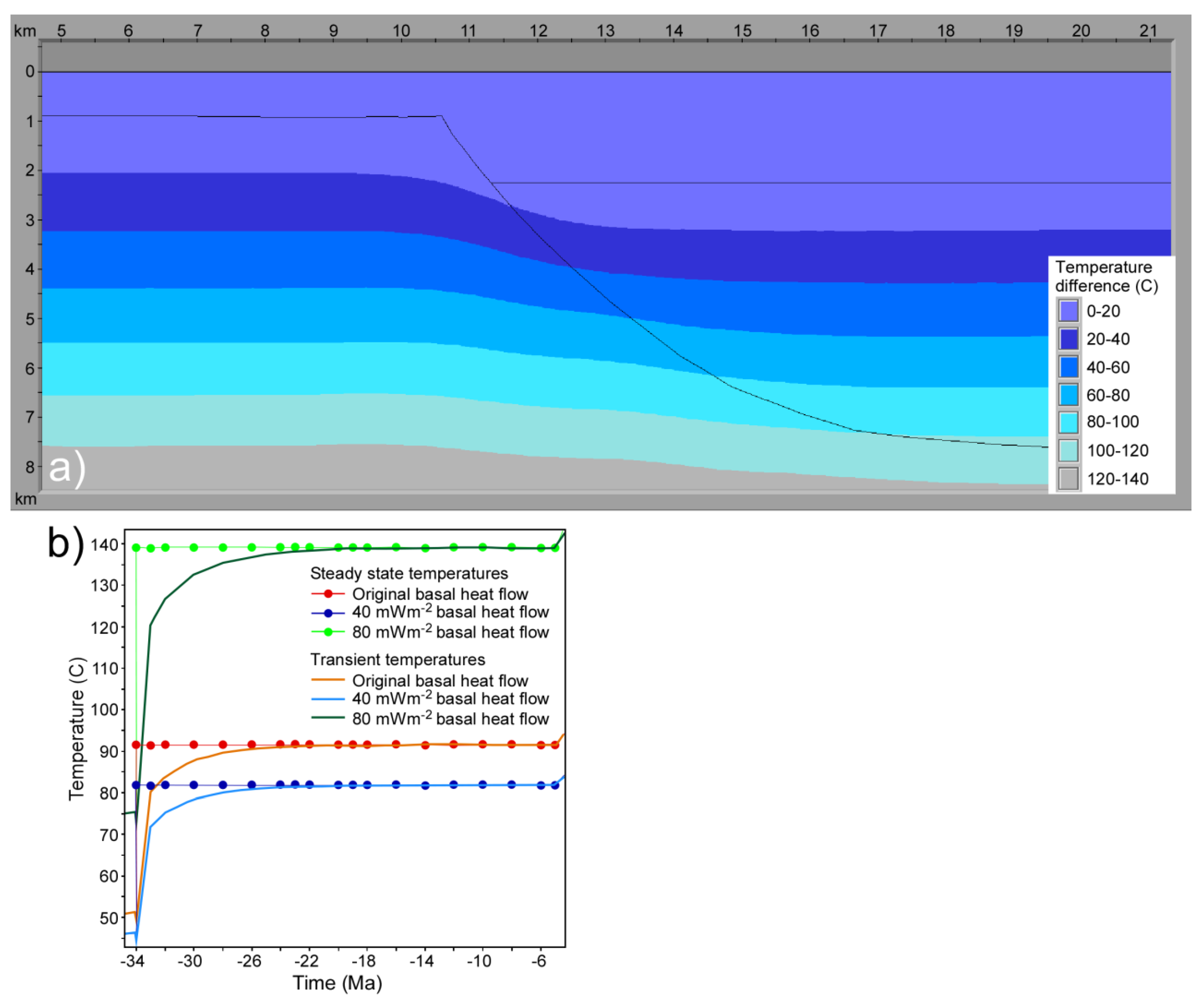
3.1.5. Basal Heat Flow

The basal heat flow, which is the heat sourced from the mantle, transferred through the basin and constitutes the lower boundary condition in the models, is so far kept constant at 47 mW·m−2. This basal heat flow value is slightly above one heat flow unit and is typical for some continental shelves, e.g., parts of the Norwegian Continental Shelf. However, to study the influence of the basal heat flow on the temperature development in the basin, three additional values were tested: 40 mW·m−2, 60 mW·m−2, and 80 mW·m−2 (Table 1). Figure 13b shows the results for 40 and 80 mW·m−2 together with the default heat flow (47 mW·m−2). Increased heat flow leads to higher steady-state temperatures and longer time is therefore needed for the basin to regain steady state (Figure 13b). The resulting transient temperatures of basins modeled with 80 mW·m−2 and 40 mW·m−2 show thermal differences up to 140 °C (Figure 13a). For the tested values, the models regain steady state approximately between 9 and 12 Myr after the fault slip. Increasing basal heat flow gives higher temperatures in the basin, and as a consequence, a longer time is needed for the basin to arrive at steady state after fault slip.

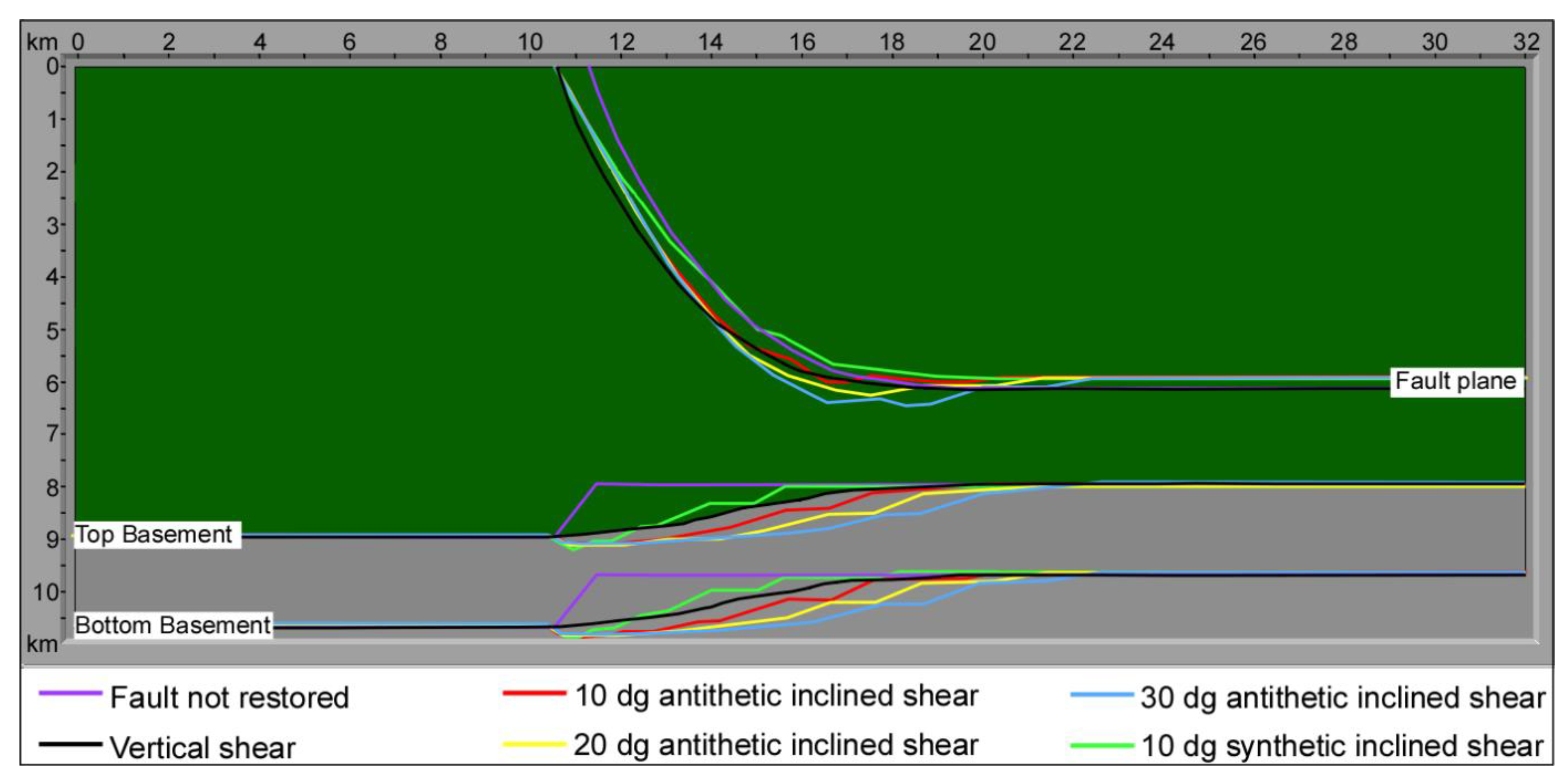
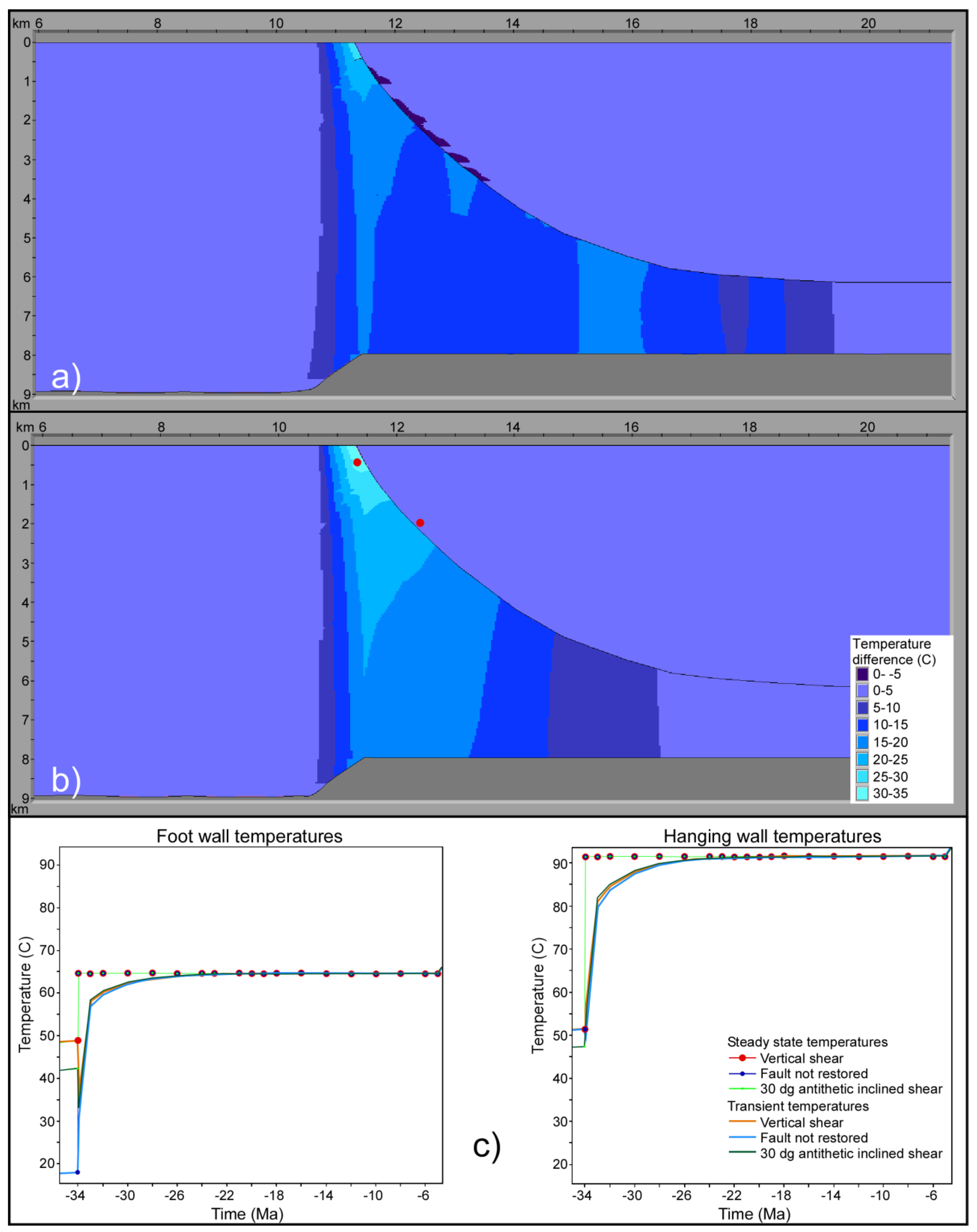
3.2. Restoration Methods

Different fault restoration methods cause different basin geometries. It is of interest to explore what effect these different geometries have on the resulting basin temperatures. In addition to vertical shear, we have therefore tested the basin reconstruction for 10° antithetic and synthetic shear, 20° and 30° antithetic shear and a case without fault reconstruction (Table 1). Basin reconstruction without fault restoration was done by moving the hanging wall section vertically up such that the timeline split by the fault zone is horizontally connected. This process gives no lateral mass movements of the basin. Vertical simple shear modeling was, as mentioned in the method section, done by BMT, while the alternative fault reconstructions were performed with Move. Antithetic simple shear results in a wider basin (Figure 2) and the larger the angle, the wider the basin. Synthetic simple shear results in a narrower basin (Figure 2 and Figure 14) relative to the other methods. Vertical simple shear falls in between these two, while basin reconstruction without fault restoration results in a geometry which is quite different from the other restored scenarios. Figure 14 shows the resulting geometries of the fault plane and top and bottom basement after fault slip of the six tested reconstruction methods. The basins with non-restored fault and restored by 10° synthetic inclined shear (purple and green line respectively, Figure 14) result in the shallowest hanging wall and top basement.
The geometry variations resulting from the tested restoration methods involve varying footwall and hanging wall area and burial depth, which result in differences in the thermal calculations, especially in the footwall section. Therefore, the thermal differences between them are concentrated in the footwall part of the basin at the time of fault slip (Figure 15). Figure 15c shows that the temperatures prior to fault slip show a larger difference on the footwall side compared to the hanging wall side. The comparison between the non-restored basin to basin restored by 30° antithetic shear, shows the largest area with thermal differences (Figure 15a), while the thermal differences between vertically- and non-restored basins are the most pronounced (Figure 15b). Although the thermal differences do not last long, ~1 Myr, such temperature differences might play a role concerning timing of generation and ultimately migration of hydrocarbons. For this particular case, the modeled thermal differences result in up to 40% maturation difference of the potential organic matter in a limited time and area of the footwall section (not shown here). All the tested restoration methods require approximately 10 Myr to achieve a steady state after fault slip. We therefore conclude that the tested restoration methods do not lead to large differences in time needed for the basins to achieve steady state. However, temperature differences due to different restoration methods may lead to temperature variations that might influence the maturation calculations.

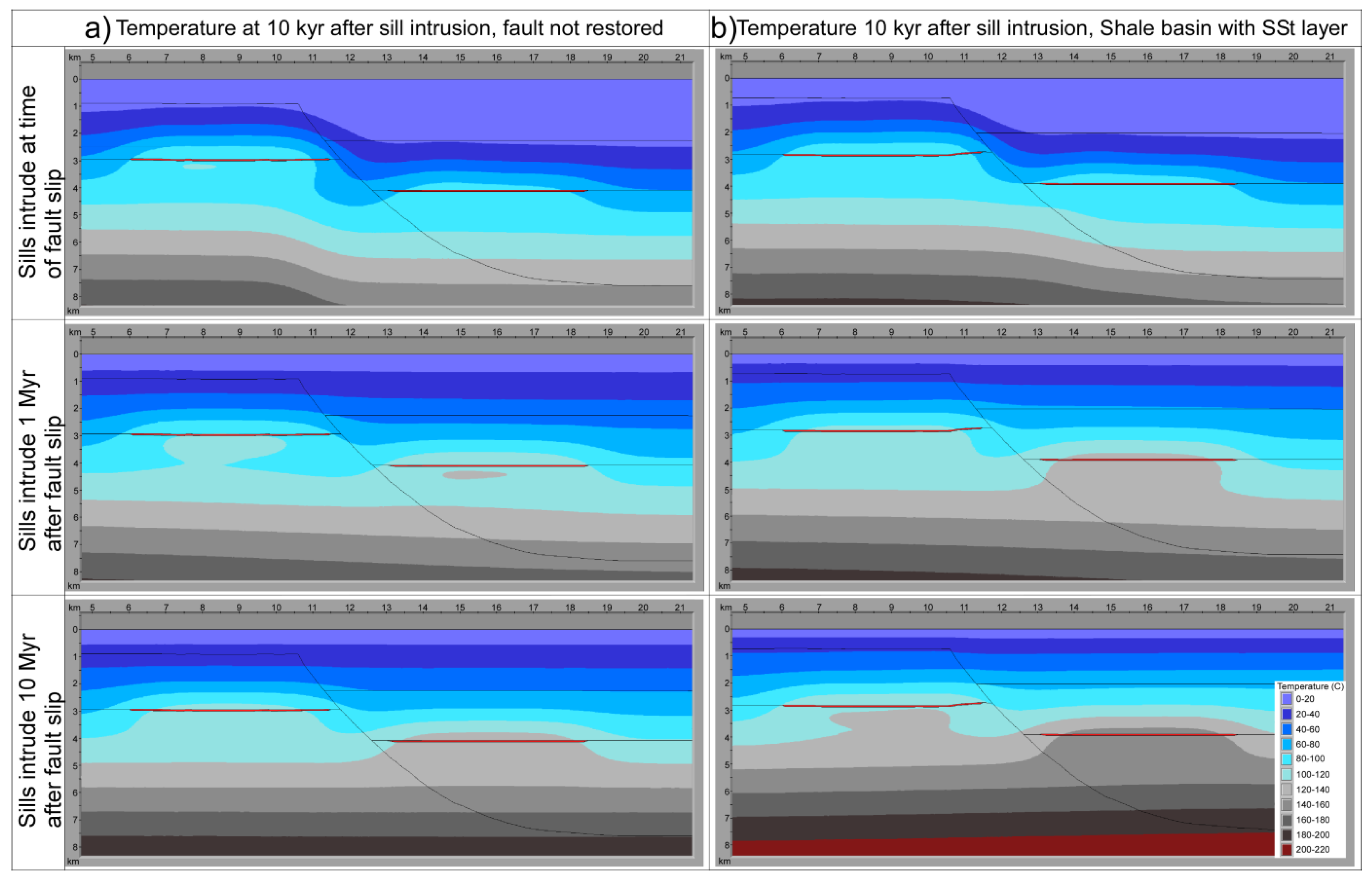
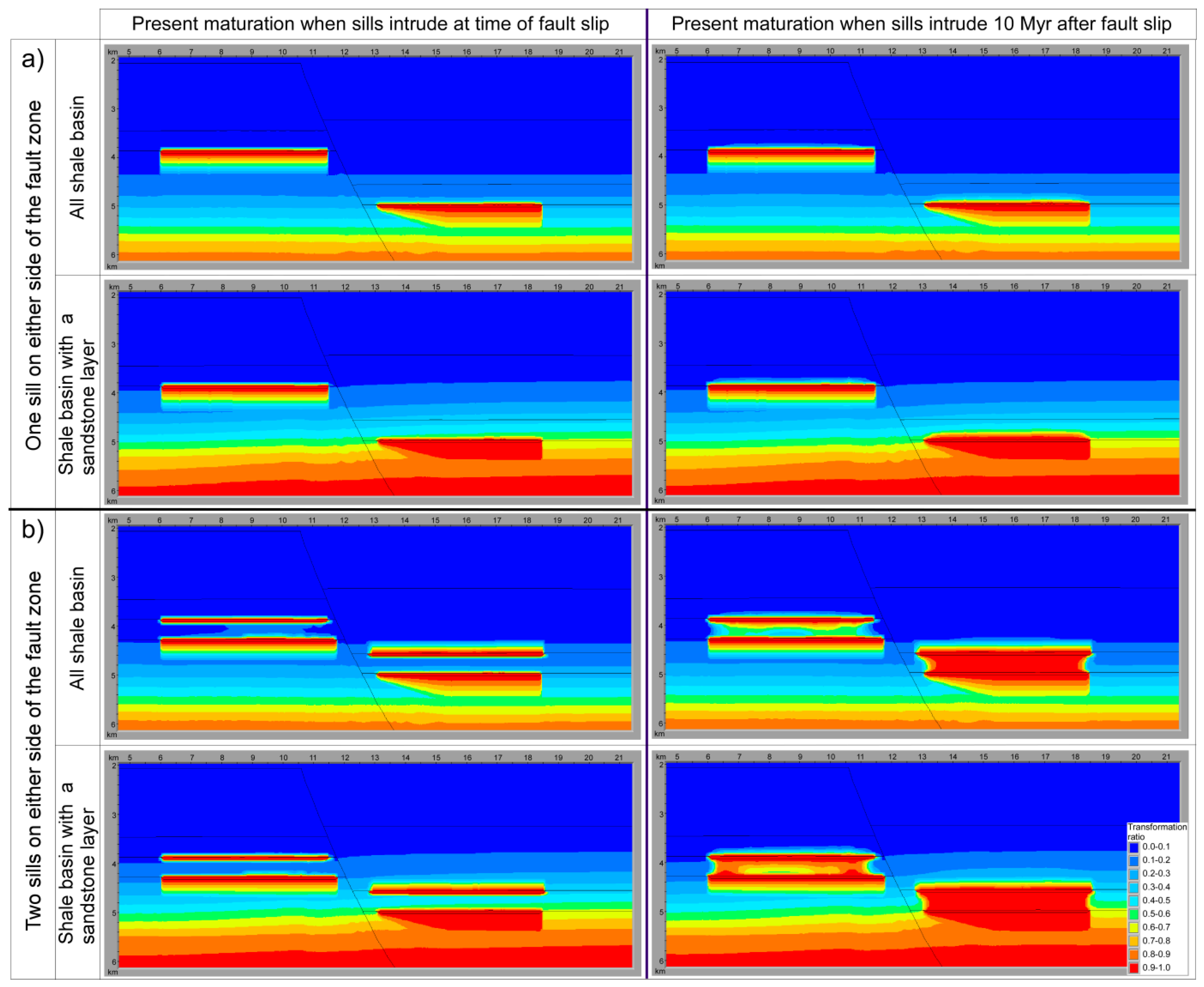
3.3. Sill Intrusions in the Basin

As mentioned above, earlier studies have pointed out the importance of host-rock temperatures at time of emplacement for the resulting thermal effects of intrusions [8,13,16,17,18]. In our study two sills, ~50 m thick, one in the hanging wall and one in the footwall, have been modeled to intrude the basin with increasing time lapse after fault slip. Figure 16 shows the results for sills intruding at time of fault slip, 1 Myr and 10 Myr after fault slip. There is a clear thermal instability on both sides of the fault zone. However, due to the masses of faulted rock and larger deposits of sediments in the hanging wall section, the thermal effects of the fault displacement are more pronounced here. Therefore, the largest differences in the thermal effects of the sills as time passes are expected to be found here.
At the time of intrusion, the temperatures in the close proximity of the sills increases dramatically (cf., [25]). As time passes the area with increased temperatures grow and consequently the temperatures starts to fall. The thermal effect of sills has a quick rise and fall within the first 1 Myr after intrusion.
Modeling results at 1000 years after fault slip show that there is a temperature difference up to 40 °C on either side of the fault zone (Figure 4). Results also show that as time passes the basin regains steady state (Figure 6a–c), which for most scenarios in this study occur somewhere between 3 and 22 Myr after fault slip. For sills intruding at time of fault slip the host-rock temperature effects are lower compared to sills intruding into a basin with a time lapse after fault slip, which have temperatures closer to that of a basin in steady state. A consequence is that sills intruding with a time lapse in relation to fault slip have higher background temperatures and the thermal effects will be more prominent (Figure 16). These thermal differences are still present 100 kyr after sill intrusion. In the hanging wall there is a temperature difference around 40 °C between the cases where the sills intrude at time of fault slip and 10 Myr after fault slip (Figure 16). The highest potential host-rock temperature effect of intruding sills will be in a steady state basin.
The largest thermal differences between basins with faults restored in different ways, was found between basin with fault restored by vertical shear to basin with non-restored fault (Figure 15b). Therefore, we have tested the possible influence of a non-restored fault basin with sills on the calculated thermal effects. As the thermal differences between a basin restored by vertical shear to a basin with a non-restored fault was found in the footwall part of the fault zone (Figure 15b), this is also the area where it is expected that possible differences in thermal effects of sills will be found (Figure 17a). However, the thermal results of the basin with sills and non-restored fault show very small thermal differences from basin with sills and fault restored by vertical shear (Figure 16 and Figure 17a). The most pronounced thermal difference is found between the scenarios where sills intrude 1 Myr after fault slip. These small temperature differences will not significantly influence the maturation calculations for the two scenarios.
Sedimentary basins worldwide normally consist of changing layers of different lithologies with contrasting properties. A homogeneous shale basin with a lower thermal conductivity, such as the average conductivity used in this study (Table 2), result in a warmer basin (Figure 10a,b) and consequently gives a higher host-rock temperature effect for intruding sills. This emphasizes that the basin lithologies and their thermal conductivities have large influence on the temperatures in the basin. We have here tested a case where the sills intrude into a shale basin with a sandstone layer (Figure 12a). The results show no differences for the sills intruding into the basin at time of fault slip (Figure 17b). However, as time passes (1 Myr and 10 Myr after fault slip) the presence of the sandstone layer makes a difference in the resulting thermal effects of the sill intrusions. Sills intruding 10 Myr after fault slip cause thermal differences in some areas up to 20 °C in both the footwall and hanging wall 10 kyr after sill intrusion (Figure 16 and Figure 17b).
As the results in Figure 16 and Figure 17 show, the thermal impact of sill intrusions are more pronounced when emplaced into a basin closer to thermal steady state. This more pronounced thermal impact also influences to a small degree the maturation levels around the sills, especially the area above the sills in the hanging wall (Figure 18a). Reports from onshore and offshore sedimentary basins with magmatic intrusions show that sills often occur in clusters (e.g., [6,9,52,67]). It is considered that multiple sills intruding at different levels within a certain time frame thermally impacts a larger rock volume of the basin compared to one single intrusion (e.g., [8,21,68]). To replicate a basin with clusters of sills, two more sills have been added to the model, one on either side of the fault zone. The thermal effect of sill swarms intruding with different timing relative to fault slip have a large impact on the matured organic material, particularly in the area between the sills on both sides of the fault zone (Figure 18b). In the heterogeneous basin, the warmer host-rock temperatures compared to the homogeneous basin, result in more transformed organic material on both sides of the fault zone for sills intruding at time of fault slip, as well as for sills intruding 10 Myr after fault slip. However, the maturation differences between the homogeneous and heterogeneous basins are more prominent when the sills intrude 10 Myr after fault slip (Figure 18b).

4. Discussion

The purpose of this work was to study the transient thermal effects in structurally complex basins with normal faults and sill intrusions. To uncover trends of several parameters transient thermal effects in sedimentary basins, both extreme and realistic values were tested. Three specific cases were addressed: the transient thermal effects of normal faulting, the ultimate effect of fault restoration method on thermal modeling, and the impact of sill intrusions in structurally complex basins. Interesting effects were discovered and are discussed separately in the following.

4.1. Transient Thermal Effects in Relation to Normal Fault Slip

Figure 4 shows that the geothermal gradient, especially in the hanging wall, changes abruptly after fault displacement and with time the basin arrives at a thermal steady state (Figure 6). The isotherms in the footwall are somewhat affected by down-faulted colder rocks and deposition of colder sediments in the hanging wall, which is in accordance with the work by ter Voorde and Bertotti [29]. By preserving a constant heat flow from the basement the model has been simplified which is acceptable as it does not change the relative differences between compared scenarios. A constructed synthetic profile has been used to uncover the thermal effects of normal faulting in structurally complex basins. Steady state is regained 3–22 Myr after the fault slip, but the time elapsed for the tested parameters and model runs to achieve this varies considerably: for fault displacement 9–11 Myr, thermal conductivity 3–22 Myr, specific heat capacity 8–18 Myr and basal heat flow 9–12 Myr. For the remaining tested parameters (Table 1) the variation of time needed to restore steady state is much smaller between the tested values, only some 100 kyr.
The syn- and post-rift deposits (Figure 1) in the studied section are 1800 m thick. These sediments are modeled to be deposited over five different time spans (Table 1); 20, 10, 5, and 1 Myr and 10 kyr, which correspond to a sedimentation rate of 0.09–180 mm·year−1. The sedimentation rate roughly overlaps the reported sedimentation rates (0.4–100 mm·year−1 for the referenced papers) (e.g., [69,70,71,72,73,74,75]). ter Voorde and Bertotti [29] suggest that the extension rate somewhat controls the thermal effect of sediment deposition. They argue that high sedimentation rates will temporarily cool the basin while low sedimentation rates lead to heating. According to their study the “turning points” are at sedimentation rates of 2.0, 2.2, and 1.4 mm·year−1 for shale, siltstone, and sandstone, respectively. Our results show that sedimentation rates > 0.18 mm·year−1 for shale result in basins with transient thermal effects, in agreement with results reported by Ehlers et al. [34]. The numerical temperature model is different in the two studies. Additionally, the resolution of the finite difference grid is much finer in our study as the focus is on a smaller part of the basin compared to the work by ter Voorde and Bertotti [29]. These elements may possibly be the reason for the different results.
All the tested deposition time spans ≤10 Myr for the syn- and post-rift sediments regain steady state approximately 10 Myr after fault slip. However, there is a difference of 600 kyr for regaining steady state between the modeled scenarios. When faulting and deposition occur over a time span of 10 Myr, steady state is restored 200 kyr after the fault slip ceased. Basins with faulting and deposition over a time span of 10 kyr and 1 Myr, regains steady state after 9.6 and 9.7 Myr, respectively. Although the compared models keep the basin in an unstable thermal condition over approximately the same time span, the slow rate of faulting and deposition makes the thermal instability less prominent as opposed to basins with a high rate of faulting and deposition (Figure 8). This coincides with the result for the models were the fault displacements are varied. The larger the fault slip, the larger the thermal differences on either side of the fault zone (Figure 7), which results in longer time required for the basin to regain steady state. For basins with faulting and deposition occurring over >10 Myr, the basin is close to, or in, steady state throughout the whole deposition process; this is in accordance with Bertotti and ter Voorde [30] and ter Voorde and Bertotti [29].
In addition, our calculations show that there is a 40 ºC difference after fault slip from one side of the fault zone to the other. Larger temperature differences have been reported in the literature, e.g., by Graseman and Mancktelow [76] (and references therein) who observed differences above 100 °C on either side of the Simplon Fault Zone in Switzerland. Although such a high difference may not be enough to cause regional disturbances in the geothermal field [30], it can lead to significant local maturation differences of deposited organic material if such thermal differences occurred in basins of sedimentary rocks. Since the oil window typically lies between 80 and 150 °C [77], some tens of degrees difference in temperature may thus lead to different stages of organic maturation on either side of a fault zone. The maturation calculations in BMT follow the Arrhenius equation, which ties the reaction rates of kerogen to the temperature differences and the activation energies of the kerogen type. For given activations energies and temperatures, the reaction rates of kerogen are roughly doubled for every 10 °C rise (e.g., [39]). This indicates that a 10 °C difference will have implications for the estimated maturation in the basin.
Figure 10 demonstrates the importance of the thermal conductivity for the obtained temperature levels in the basin. Worldwide basins show a variety of alternating lithologies, and consequently differences in thermal conductivities [38,63]). Our modeling shows that thermal conductivity, as well as the fault movement, influence both the steady state and the transient temperatures in the basin (Figure 12), and therefore the time needed to regain steady state. This is in keeping with results reported by Fjeldskaar et al. [78] who demonstrated the need for an accurate description of the thermal-conductivity variation to obtain a correct thermal history, on which the prediction of maturation is based.
The thermal conductivity of lithologies, amount of fault slip, time span of faulting and deposition, angle of fault zone, and basal heat flow will influence both the size of the affected area and level of the thermal imbalance. Specific heat capacity will determine the time needed for a basin to regain steady state (Figure 11) [26,35].

4.2. Fault Restoration and Its Effect on Thermal Modeling

Hydrocarbons are often trapped in structurally complex basins, yet structural reconstruction is often over-simplified in traditional basin modeling [26]. We have shown that the tested restoration methods do not lead to substantial differences in the thermal estimates. Dula [40] concludes that 20 degrees antithetic simple shear result in a geometry resembling the natural basin the most. However, resulting thermal calculations for vertical shear and 20 degrees antithetic shear show negligible differences. We therefore conclude that thermal estimates of transects restored by vertical shear give reasonable results.
The largest thermal differences are found between basins with the greatest deviation in restored geometry and, consequently, deviation in burial depth. Thermal differences up to 35 °C are found when the temperatures obtained for basin restored by vertical shear are compared to basin with non-restored fault. Fjeldskaar et al. [26] demonstrated the importance of fault reconstruction for the temperature modeling on a 2D section from the Gulf of Mexico. Up to 70 °C in temperature differences were observed in the footwall part of the basin between model with reconstructed faults versus model with no fault reconstruction. This strongly suggests that accounting for the structural evolution in sedimentary basins is essential for a reliable thermal and maturation modeling. The results from this study along with those of Fjeldskaar et al. [26] emphasize the importance of proper structural reconstruction of sedimentary basins and highlights the need to study the transient thermal effects that occur in a basin proceeding a fault slip in order to make good thermal and maturation estimates.

4.3. Fault Slip and Magmatic Intrusions

As mentioned above, the pre-intrusion host-rock temperatures are acknowledged to be important for the thermal effect of magmatic intrusions and the size of the thermal aureole (e.g., [8]). Fault slip and magmatic intrusions may occur within the same timeframe (e.g., [30,64,65]). Results in this study show that the thermal effects of magmatic intrusions are sensitive to the timing of the fault slip relative to the timing of the sill emplacement (Figure 16, Figure 17 and Figure 18). The basin with no sills shows that millions of years are required to restore steady state after fault movement (Figure 5 and Figure 6). Before fault slip, sediments in the hanging wall are buried at shallower depths in the basin compared to after fault slip. The cold sediments in the hanging wall will gradually experience a temperature increase up to 40 °C over a time span of ~10 Myr. With warmer host-rock temperatures the thermal effect of intrusions is higher. Figure 8, Figure 10, Figure 11 and Figure 12 show temperature histories as a function of various parameters with time to equilibrium of several Myr. However, temperatures rebound within 1 Myr or less to only a few degrees from steady state temperatures. Sedimentary basins in general would possibly not show variation in maturation due to transient thermal effects over ~1 Myr. Unless, the thermal differences were of a certain magnitude, as the reaction rates of kerogen is doubled for every 10 °C rise (e.g., [39]) as mentioned above. Sydnes et al. [25] show that the main thermal effect of magmatic sill intrusions occurs within the first 1 Myr after intrusion. This indicates that if faulting and sill intrusion occurs within the same timeframe, two transient thermal effects operate simultaneously in the basin. Disregarding these transient thermal effects could possibly lead to over- or underestimation of the basin maturation.
Sills intruding around the time of fault slip are emplaced into a basin with lower background temperatures than sills intruding 10 Myr after fault displacement. However, these differences in host-rock temperatures lead to larger thermal effects (Figure 16), as mentioned above, but do not result in large differences in maturation of organic material when one sill intrudes on both sides of the fault zone (Figure 18a). This is in contrast to the results of Aarnes et al. [8] who concluded that the host-rock temperature is an important parameter in relation to aureole thickness and thus the amount of generated gas after intrusion of one sill. They found that increasing the host-rock temperature by 50 °C has a larger impact on the aureole thickness than both the option of increasing the temperature of the intruding magma by 50 °C or by increasing the sill thickness by 50 m. They also found that thinner sills have smaller thermal aureoles than thicker sills [8]. In this study ~50 m thick sills have been used as opposed to the work by Aarnes et al. [8], who studied a 100 m thick sill. This difference in sill thickness might possibly be the reason for the different conclusions in these two studies.
As for sill clusters, a 40 °C difference in background temperature results in a larger area with matured organic material around the intruded sills (Figure 18b). This is in agreement with Aarnes et al. [21] and Sydnes et al. [25] who showed that the thermal aureole of sill clusters at multiple levels thermally impacts a larger volume of surrounding rocks than single sills. Both these studies also show that sill thickness plays a role in the thermal and maturation effects. A 100 m thick sill will mature organic material in a larger rock volume than a thinner sill [21,25].
Figure 10 shows clearly that the thermal conductivity plays a significant role for the obtained basin temperatures. The results of sills intruding into a heterogeneous shale basin with a sandstone layer has a greater thermal effect on the surrounding host rocks, and is especially visible for sills intruding 10 Myr after fault slip (Figure 17). With the presence of higher thermal conductivity lithologies the host-rock temperatures increases and the thermal and maturation effect of magmatic intrusions are enhanced (Figure 18a,b), a conclusion supported by others (e.g., [8,16,21]).

4.4. Limitations of the Study

4.4.1. Assumptions

A simple model with one listric fault and one faulting event has been used in this study. The layers end horizontally in the fault zone and most of the tested scenarios assume a homogeneous lithology. Deposited sediments are modeled to reach the surface in every timestep, meaning that there are no constraints on the sediment supply and sea level is not accounted for. The magmatic sill intrusions are modeled to be horizontal and concordant to the layering with a constant sill thickness. Natural basins commonly consist of several faults, several faulting events, and different fault dips possibly dipping in various directions. Furthermore, layers often show a bending downwards towards the fault zone of a listric fault and they commonly show a large lithological heterogeneity, which might lead to a variation in physical properties. All these factors may result in variations in the estimated transient thermal effects and the time needed for the basin to regain steady state after fault slip, and contribute to contrasting host-rock temperatures. The occurrence of salt in the vicinity of sills will in particular influence the thermal situation in basins. Including all the above mentioned factors is possible and will turn the model into a more realistic example. However, doing so will limit the general conclusions that can be drawn from our study. By keeping the model simple the study is focused on fundamental questions related to transient thermal effects in basins with normal faults and magmatic sills. Revealed trends in this study are therefore applicable for basins in general with such features, as the relative differences between the tested parameters will remain more or less the same.
Sills vary normally in thickness and shape, e.g., saucer-shaped, v-shaped, and transgressive sills (cf., [67,79,80]). Sill thickness influences the temperature effects in the surrounding area; a thick magmatic sill has a wider thermal influence on the surroundings than a thin sill. It influences the size of the thermal aureole surrounding it (e.g., [8,25]) and an uneven sill thickness could possibly lead to an uneven thermal aureole. In a 2D model, the intrusion is extended infinitely in the 3rd direction. This is a good approximation as sills commonly have much larger horizontal dimensions compared to the vertical dimension. The sills are often several km in lengths and widths, while possibly only 50–100 m thick. For typical sill dimensions, the 2D modeling is sufficient for realistic temperature calculations. Fjeldskaar et al. [7] studied the 3D effect of magmatic sill intrusions and investigated what length/width ratio of the sill that requires a 3D calculation to give realistic temperature results.
In the temperature modeling the initial temperature of the intruding magma is set to 1000 °C and latent crystallization heat is not accounted for. Most magmas have temperatures ranging from 700 to 1300 °C (cf., [81] and references therein) making the chosen temperature in this study a mean value. Higher magma temperatures will increase the thermal effects of the sills, whilst a lower magma temperature will have the opposite effect. However, the relative differences between the compared models in this study will stay the same, as the intruding magma initial temperature is constant in all models.
Magmatic sills are often fed by dykes in magmatic upwelling zones. These near vertical features will contribute with additional heat to the thermal history of basins with sills. However, magmatic sills can also be fed by other sills over relatively large distances which has been observed in the field (e.g., [52]).
Latent heat of crystallization is thermal energy released when the sill undergoes a phase transition from liquid to solid. The composition of the magma may differ, which may lead to different timing of the emissions of latent heat as components have different crystallization temperatures. Peace et al. [62] have estimated the additional latent heat to be 488 °C, which is a substantial thermal contribution. Heat due to solidification of the magma will be released as long as the sill contains liquids and until the sill has solidified completely. However, introducing this additional heat as one pulse, either by increasing the starting temperature of the magma or introducing it as an additional heat when the sills start to cool, may result in an overestimation of the effect of sills [20].

4.4.2. Temperature Model

The temperature calculations are done by a finite difference scheme. The grid resolution is very high around magmatic sills and in areas of irregular structures. Fjeldskaar et al. [7] showed that the numerical temperature results for magmatic sills match the analytical solutions quite well, both spatially and temporally. On this basis, we argue that the uncertainty of the conduction-temperature calculations is of minor importance.
In our model we assume that the sills cool by conduction, but it is possible that the process could be accelerated by convection. Water convecting in the vicinity of sill intrusions could significantly modify the temperature and maturity effect of intrusions. Convection of hot fluids from the magma, the host-rock water, and decomposition products of kerogen is dependent on the permeability of porous host rocks or hydrofracturing in less porous host rocks (cf., [60,61,82,83,84]. How the fluids from magma and host rock affect the fluid pressure and flow is determined by the host-rock porosity, permeability, and amount of fluids present [85]. Wang and Manga [83] showed that for rocks with low permeability (<10 mD) symmetrical contact aureoles are produced, implying that conduction is the favorable cooling method for sills and host rocks after emplacement. On the other hand, rocks of high permeability (>50 mD) show maturation asymmetry above the sill, implying occurrence of convection-influenced maturation [83]. Annen [84] studied the maximum temperatures of three rocks of different water saturations: dry, hydrated and total water saturated, and found that in close proximity to an intrusion (~10 m) there were no differences in the temperatures, whereas at a distance of 50 m there was a ~50 °C maximum temperature difference. Dry rock has the highest temperature and water saturated rock the lowest. This means that convection of water lowered the temperature by ~50 °C. It was concluded that diffusivity contrasts between magma and host rock and incremental sill emplacement had more effect on the aureole thickness than host-rock water content [84]. For the present study this implies that for highly porous and permeable lithologies (e.g., sandstone) the predicted time for cooling might be overestimated. However, for less porous and permeable lithologies (e.g., shale) the estimated cooling rates would be adequate. This was also shown by temperature and maturity modeling on data from offshore Norway [7].
Another aspect of convection, is the possible increased permeability that occurs when sills are emplaced. Sill emplacement may potentially induce stresses high enough on the surrounding host rocks to reactivate or produce new shear fractures or open up tensile fractures (e.g., [86,87]), allowing for increased permeability and possibly increased convection. However, accumulation of stresses and reactivation and/or production of faults and fractures are highly area specific and dependent on, e.g., the lithology, deformation features and existing weakness zones. Although increased convection due to emplacement of sills have been identified on seismic images (e.g., [67]) it is too area specific to be included in a study aiming for some general conclusions.
Radioactive decay within the sedimentary section itself can generate heat, but is not accounted for in this study. Rybach [88] found, however, that the contribution of radioactivity in the sedimentary section was generally no more than a few percent of the overall heat budget, which support that the errors by not accounting for radioactive heat, is insignificant. Others have concluded for the opposite and advocate for including radiogenic heat production in the thermal history modeling (e.g., [89,90]), but also emphasize the large area-variations in radiogenic heat production for the same lithologies [90].
Frictional heating from fault displacement may potentially have implications for the thermal history in a basin. ter Voorde and Bertotti [29] calculated for shear stress of 100 MPa and an extension rate of 2 mm·year−1 that the thermal contribution from frictional heat would be 2.5 °C. They concluded that this could not influence the thermal situation in the basin to a significant degree. However, with higher extensional rates and larger shear stress the frictional heating may become important.

4.4.3. Kerogen Type

Simulations of kerogen maturation can only be as good as the kinetic parameters used in the model. The parameters are derived from laboratory experiments, and are assumed to be applicable to geological processes although the scales are different by orders of magnitude. Thus the uncertainty in the calculated maturity can be significant.
As mentioned above, the maturation modeling in our study assumes kerogen type II, which is considered to be the most abundant among marine shales [39]. Kerogen degradation is temperature dependent following the Arrhenius law (e.g., [39,63]). Due to kerogen types having different activation energies, reaction rates of other kerogen types in the models presented here, could result in different maturity effects in the modeled scenarios.

5. Concluding Remarks

We have studied the transient thermal effects in a constructed basin with magmatic sill intrusions and one normal faulting event. Several factors related to faulting, physical properties, and fault restoration methods have been tested to study possible differences in resulting calculated temperature regimes over time. Sills of modest sill thickness (50 m) have been modeled to intrude before the basin has regained steady state after fault slip, enabling the study of two transient thermal effects acting simultaneously in the basin.
From the results in this study, the following conclusions can be drawn:
  • After fault slip, the basin is thermally unstable and is influenced by transient thermal effects that may last up to several million years. This implies that transient thermal effects should be accounted for if sills are emplaced after the structural events, as they might affect the pre-intrusion host-rock temperatures.
  • With increasing fault displacement, the temperature effects of fault slip on either side of the fault zone increases, as does the time the basin is thermally unstable.
  • For faulting and deposition occurring over a time span of more than 10 Myr, the basin is in, or close to, a steady state throughout the entire period. However, for the same basin, but with faulting and deposition occurring over less than 10 Myr, the basin is thermally unstable for ~10 Myr. This means that the shorter the time used on faulting and deposition, the longer is the time the basin is thermally unstable.
  • Different fault angles barely influence the time the basin is in a transient state. All tested angles lead to steady state ~10 Myr after fault slip. However, different fault angles cause changes in the foot wall and hanging wall areas and thus affect the host-rock temperature and therefore the temperature effect of potential sills.
  • Thermal conductivity is the parameter influencing pre-intrusion host-rock temperatures in the basin the most. As temperatures increase, so does the time needed for the basin to regain steady state after fault slip. For basins with identical temperature regimes, the specific heat capacity is the important property determining the time needed for the basin to regain steady state.
  • The obtained temperatures in the basin increase with increasing basal heat flow, thereby increasing the time needed to arrive at a steady state after fault slip.
  • Different restoration methods result in basins of different geometries, leading to temporary thermal differences mainly in the footwall part of the basin. The largest thermal differences are found between basins with fault restored to basin with non-restored fault.
  • Disregarding transient thermal effects proceeding normal fault slip may lead to both under- or overestimation of pre-intrusion host-rock temperature. This will influence the calculated effects of intruded sills and has implications for the estimate of how magmatic intrusions influence hydrocarbon maturation and is particularly the case for sills intruding as clusters at multiple levels.
  • A basin that has regained steady state after normal faulting has the highest potential host-rock temperature.
Emplacement of magmatic intrusions may possibly affect the reservoir quality and the fault and fracture permeability in their vicinity. Future work should evolve around the effects magmatic intrusions have on the diagenetic processes in its surroundings.

Author Contributions

Conceptualization, M.S., W.F., I.G. and I.F.L.; methodology, M.S., W.F. and I.G.; validation, W.F.; investigation, M.S..; writing—original draft preparation, M.S..; writing—review and editing, W.F., R.M., I.G. and I.F.L.; visualization, M.S. and I.G..; supervision, W.F. and R.M..; project administration, I.F.L..; funding acquisition, I.F.L.

Funding

This research was partly funded by The Research Council of Norway and Tectonor AS as a part of the PhD project ‘Effects of magmatic intrusions on temperature history and diagenesis in sedimentary basins—and the impact on petroleum systems’, RCN project number 257492.

Acknowledgments

We want to express gratitude for the support. The authors acknowledge the use of the Move Software Suite granted by Petroleum Experts Limited. Nestor Cardozo is thanked for fruitful discussions throughout the course of designing the study. Craig Magee is thanked for providing helpful comments and three anonymous referees are thanked for constructive reviews.

Conflicts of Interest

The authors declare no conflict of interest.

Appendix A

Numerical temperature model,
The following equation is discretizised,
x K h T x + z K v T z =   t ( c T )
where T is the temperature, Kh is the horizontal conductivity, and Kv is the vertical conductivity. Finite differences and a cell-centered grid are used. In the block with indices (ij) the expression
z K h T z
is evaluated by the following formula [91]:
[ x K h T x ] i j = 1 δ x i [ K h i + 1 2 , j ( 2 ( T i + 1 ,   j T i , j ) δ x i + δ x i + 1 ) K h i 1 2 , j   ( 2 ( T i , j T i 1 , j ) δ x i 1 + δ x i ) ]
K h i + 1 2 , j is the value of Kh at the boundary between the blocks (i,j) and (i + 1,j). It is computed as the harmonic mean of Khi,j and Khi + 1,j.
The expression z K v T z is treated analogously.
This gives M   ·   N equations to find the Ti,j, unknowns, where i = 1,2,…,M, j =1,2,…,N. Here, M and N are the number of blocks in x-direction and z-direction, respectively.
We use both Dirichlet and Neumann boundary conditions for the temperature model. For Dirichlet boundary conditions the temperature, T, at the boundary is given whereas for Neumann conditions the heat flux, K h T x and K v T z , is given. A Neumann boundary condition with a heat flux of zero is used for the basin edges.
An iterative method is used to solve the linear system. Conjugate gradients are used as an acceleration method [92,93]. The conjugate gradient method is preconditioned by nested factorization [94].

References

  1. Schutter, S.R. Occurrences of hydrocarbons in and around igneous rocks. In Hydrocarbons in Crystalline Rocks; Petford, N., McCaffrey, K.J.W., Eds.; Geological Society, Special Publications: London, UK, 2003; Volume 214, pp. 35–68. [Google Scholar]
  2. Zou, C.; Zhang, G.; Zhu, R.; Yuan, X.; Zhao, X.; Hou, L.; Wen, B.; Wu, X. Volcanic Reservoirs in Petroleum Exploration: Petroleum Industry Press; Elsevier Inc.: Amsterdam, The Netherlands, 2013. [Google Scholar]
  3. Senger, K.; Planke, S.; Polteau, S.; Ogata, K.; Svensen, H. Sill emplacement and contact metamorphism in a siliciclastic reservoir on Svalbard, Arctic Norway. Nor. J. Geol. 2014, 94, 155–169. [Google Scholar]
  4. Schutter, S.R. Hydrocarbon occurrence and exploration in and around igneous rocks. In Hydrocarbons in Crystalline Rocks; Petford, N., McCaffrey, K.J.W., Eds.; Geological Society, Special Publications: London, UK, 2003; Volume 214, pp. 7–33. [Google Scholar]
  5. Svensen, H.; Planke, S.; Malthe-Sørenssen, A.; Jamtveit, B.; Myklebust, R.; Eidem, T.R.; Rey, S.S. Release of methane from a volcanic basin as a mechanism for initial Eocene global warming. Nature 2004, 429, 542–545. [Google Scholar] [CrossRef] [PubMed]
  6. Svensen, H.; Planke, S.; Corfu, F. Zircon dating ties NE Atlantic sill emplacement to initial Eocene global warming. J. Geol. Soc. 2010, 167, 433–436. [Google Scholar] [CrossRef]
  7. Fjeldskaar, W.; Helset, H.M.; Johansen, H.; Grunnaleite, I.; Horstad, I. Thermal modelling of magmatic intrusions in the Gjallar Ridge, Norwegian Sea: Implications for vitrinite reflectance and hydrocarbon maturation. Basin Res. 2008, 20, 143–159. [Google Scholar] [CrossRef]
  8. Aarnes, I.; Svensen, H.; Connolly, J.A.D.; Podladchikov, Y.Y. How contact metamorphism can trigger global climate changes: Modeling gas generation around igneous sills in sedimentary basins. Geochim. Et Cosmochim. Acta 2010, 74, 7179–7195. [Google Scholar] [CrossRef]
  9. Svensen, H.; Corfu, F.; Polteau, S.; Hammer, Ø.; Planke, S. Rapid magma emplacement in the Karoo Large Igneous Province. Earth Planet. Sci. Lett. 2012, 325–326, 1–9. [Google Scholar] [CrossRef]
  10. Moorcroft, D.; Tonnelier, N. Contact Metamorphism of Black shales in the Thermal Aureole of a dolerite sill within the Karoo Basin. In Origin and Evolution of the Cape Mountains and Karoo Basin, Regional Geology Reviews; Linol, B., de Wit, M.J., Eds.; Springer International Publishing: Cham, Switzerland, 2016; pp. 75–84. [Google Scholar]
  11. Othman, R.; Arouri, K.R.; Ward, C.R.; McKirdy, D.M. Oil generation by igneous intrusions in the northern Gunnedah Basin, Australia. Org. Geochem. 2001, 32, 1219–1232. [Google Scholar] [CrossRef]
  12. Monreal, F.R.; Villar, H.; Baudino, R.; Delpino, D.; Zencich, S. Modeling an atypical petroleum system: A case study of hydrocarbon generation, migration and accumulation related to igneous intrusions in the Neuquen Basin, Argentina. Mar. Pet. Geol. 2009, 26, 590–605. [Google Scholar] [CrossRef]
  13. Spacapan, J.B.; Palma, J.O.; Galland, O.; Manceda, R.; Rocha, E.; D’Odorico, A.; Leanza, H.A. Thermal impact of igneous sill-complexes on organic-rich formations and implications for petroleum systems: A case study in the northern Neuquén Basin, Argentina. Mar. Pet. Geol. 2018, 91, 519–531. [Google Scholar] [CrossRef]
  14. Wang, D.; Song, Y. Influence of different boiling points of pore water around an igneous sill on the thermal evolution of the contact aureole. Int. J. Coal Geol. 2012, 104, 1–8. [Google Scholar] [CrossRef]
  15. Wang, D.; Zhao, M.; Qi, T. Heat-transfer-model analysis of the thermal effect of intrusive sills on organic-rich host rocks in sedimentary basins. In Earth Sciences; Dar, I.A., Ed.; InTech: London, UK, 2012. [Google Scholar]
  16. Dow, W.G. Kerogen studies and geological interpretations. J. Geochem. Explor. 1977, 7, 79–99. [Google Scholar] [CrossRef]
  17. Bostick, N.H.; Pawlewicz, M.J. Paleotemperatures based on vitrinite reflectance of shales and limestones in igneous dike aureoles in the Upper Cretaceous Pierre Shale, Walsenburg, Colorado. In Hydrocarbon Source Rocks of the Greater Rocky Mountain Region; Woodward, J.G., Meissner, F.F., Clayton, C.J., Eds.; Rocky Mountain Association of Geologists Symposium: Denver, CO, USA, 1984; pp. 387–392. [Google Scholar]
  18. Raymond, A.C.; Murchison, D.G. Development of organic maturation in the thermal aureoles of sills and its relation to sediment compaction. FUEL 1988, 67, 1599–1608. [Google Scholar] [CrossRef]
  19. Aarnes, I.; Planke, S.; Trulsvik, M.; Svensen, H. Contact metamorphism and thermogenic gas generation in the Vøring and Møre basins, offshore Norway, during the Paleocene-Eocene thermal maximum. J. Geol. Soc. 2015, 172, 588–598. [Google Scholar] [CrossRef]
  20. Galushkin, Y.I. Thermal effects of igneous intrusions on maturity of organic matter: A possible mechanism of intrusion. Org. Geochem. 1997, 26, 645–658. [Google Scholar] [CrossRef]
  21. Aarnes, I.; Svensen, H.; Polteau, S.; Planke, S. Contact metamorphic devolatilization of shales in the Karoo Basin, South Africa, and the effects of multiple sill intrusions. Chem. Geol. 2011, 281, 181–194. [Google Scholar] [CrossRef]
  22. Wang, D. Comparable study on the effect of errors and uncertainties of heat transfer models on quantitative evaluation of thermal alteration in contact metamorphic aureoles: Thermophysical parameters, intrusion mechanism, pore-water volatilization and mathematical equations. Int. J. Coal Geol. 2012, 95, 12–19. [Google Scholar]
  23. Wang, D.; Song, Y.; Xu, H.; Ma, X.; Zhao, M. Numerical modeling of thermal evolution in the contact aureole of a 0.9 m thick dolerite dike in the Jurassic siltstone section from Isle of Skye, Scotland. J. Appl. Geophys. 2013, 89, 134–140. [Google Scholar] [CrossRef]
  24. Liu, E.; Wang, H.; Uysal, I.T.; Zhao, J.-X.; Wang, X.-C.; Feng, Y.; Pan, S. Paleogene igneous intrusion and its effect on thermal maturity of organic-rich mudstones in the Beibuwan Basin, South China Sea. Mar. Pet. Geol. 2017, 86, 733–750. [Google Scholar] [CrossRef]
  25. Sydnes, M.; Fjeldskaar, W.; Løtveit, I.F.; Grunnaleite, I.; Cardozo, N. The importance of sill thickness and timing of sill emplacement on hydrocarbon maturation. Mar. Pet. Geol. 2018, 89, 500–514. [Google Scholar] [CrossRef]
  26. Fjeldskaar, W.; Andersen, Å.; Johansen, H.; Lander, R.; Blomvik, V.; Skurve, O.; Michelsen, J.K.; Grunnaleite, I.; Mykkeltveit, J. Bridging the gap between basin modelling and structural geology. Reg. Geol. Metallog. 2017, 72, 65–77. [Google Scholar]
  27. Benfield, A.E. The effect of uplift and denudation on underground temperatures. J. Appl. Phys. 1949, 20, 66–70. [Google Scholar] [CrossRef]
  28. Birch, F. Flow of heat in the Front Range, Colorado. Geol. Soc. Am. Bull. 1950, 61, 567–630. [Google Scholar] [CrossRef]
  29. ter Voorde, M.; Bertotti, G. Thermal effects of normal faulting during rifted basin formation, 1. A finite difference model. Tectonophysics 1994, 240, 133–144. [Google Scholar] [CrossRef]
  30. Bertotti, G.; ter Voorde, M. Thermal effects of normal faulting during rifted basin formation, 2. The Lugano-Val Grande normal fault and the role of pre-existing thermal anomalies. Tectonophysics 1994, 240, 145–157. [Google Scholar] [CrossRef]
  31. Johnson, C.; Harbury, N.; Hurford, A.J. The role of extension in the Miocene denudation of the Nevado-Filábride Complex, Betic Cordillera (SE spain). Tectonics 1997, 16, 189–204. [Google Scholar] [CrossRef]
  32. Bertotti, G.; Seward, D.; Wijbrans, J.; ter Voorde, M.; Hurford, A.J. Crustal thermal regime prior to, during, and after rifting: A geochronological and modeling study of the Mesozoic South Alpine rifted margin. Tectonics 1999, 18, 185–200. [Google Scholar] [CrossRef]
  33. Ehlers, T.A.; Chapman, D.S. Normal fault thermal regimes: Conductive and hydrothermal heat transfer surrounding the Wasatch fault, Utah. Tectonophysics 1999, 312, 217–234. [Google Scholar] [CrossRef]
  34. Ehlers, T.A.; Armstrong, P.A.; Chapman, D.S. Normal fault thermal regimes and the interpretation of low-temperature thermochronometers. Phys. Earth Planet. Inter. 2001, 126, 179–194. [Google Scholar] [CrossRef]
  35. Lander, R.H.; Langfeldt, M.; Bonnell, L.; Fjeldskaar, W. BMT User’s Guide; Tectonor AS Proprietary Publication: Stavanger, Norway, 1994. [Google Scholar]
  36. Fjeldskaar, W. BMTTM—Exploration tool combining tectonic and temperature modeling: Business Briefing: Exploration & Production. Oil Gas Rev. 2003, 1–4. [Google Scholar]
  37. Sclater, J.G.; Christie, P.A.F. Continental stretching: An explanation of the post-mid-cretaceous subsidence of the central North Sea basin. J. Geophys. Res. 1980, 85, 3711–3739. [Google Scholar] [CrossRef]
  38. Čermác, V.; Rybach, L. Thermal properties: Thermal conductivity and specific heat of minerals and rocks. In Landolt-Börnstein Zahlenwerte und Functionen aus Naturwissenschaften und Technik, Neue Serie, Physikalische Eigenschaften der Gesteine; Angeneister, G., Ed.; Springer Verlag: Berlin/Heidelberg, Germany; New York, NY, USA, 1982; pp. 305–343. [Google Scholar]
  39. Tissot, B.P.; Welte, D.H. Petroleum Formation and Occurrence, 2nd ed.; Springer-Verlag: Berlin/Heidelberg, Germany, 1984. [Google Scholar]
  40. Dula, W.F. Geometric Models of Listric normal Faults and Rollover Folds. Am. Assoc. Pet. Geol. Bull. 1991, 75, 1609–1625. [Google Scholar]
  41. Fossen, H. Structural Geology; Cambridge University Press: Cambridge, UK, 2010. [Google Scholar]
  42. Osagiede, E.E.; Duffy, O.B.; Jackson, C.A.-L.; Wrona, T. Quantifying the growth history of seismically imaged normal faults. J. Struct. Geol. 2014, 66, 382–399. [Google Scholar] [CrossRef]
  43. Magee, C.; Maharaj, S.M.; Wrona, T.; Jackson, C.A.-L. Controls on the expression of igneous intrusions in seismic reflection data. Geosphere 2015, 11, 1024–1041. [Google Scholar] [CrossRef]
  44. Schofield, N.; Holford, S.; Millett, J.; Brown, D.; Jolley, D.; Passey, S.R.; Muirhead, D.; Grove, C.; Magee, C.; Murray, J.; et al. Regional Magma Plumbing and emplacement mechanisms of the Faroe-Shetland sill Complex: Implications for magma transport and petroleum systems within sedimentary basins. Basin Res. 2017, 29, 41–63. [Google Scholar] [CrossRef]
  45. Eide, C.H.; Schofield, N.; Lecomte, I.; Buckley, S.J.; Howell, J.A. Seismic interpretation of sill complexes in sedimentary basins: Implications for the sub-sill imaging problem. J. Geol. Soc. 2017, 175, 193–209. [Google Scholar] [CrossRef]
  46. Francis, E.A. Magma and sediment-I: Emplacement mechanism of late Carboniferous tholeiite sills in northern Britain. J. Geol. Soc. 1982, 139, 1–20. [Google Scholar] [CrossRef]
  47. Chevallier, L.; Woodford, A. Morpho-tectonics and mechanism of emplacement of the dolerite rings and sills of the western Karoo, South Africa. S. Afr. J. Geol. 1999, 102, 43–54. [Google Scholar]
  48. Galerne, C.Y.; Neumann, E.-R.; Planke, S. Emplacement mechanisms of sill complexes: Information from the geochemical architecture of the Golden Valley Sill Complex, South Africa. J. Volcanol. Geotherm. Res. 2008, 177, 425–440. [Google Scholar] [CrossRef]
  49. Galerne, C.Y.; Galland, O.; Neumann, E.-R.; Planke, S. 3D relationships between sills and their feeders: Evidence from the Golden Valley Sill Complex (Karoo Basin) and experimental modelling. J. Volcanol. Geotherm. Res. 2011, 202, 189–199. [Google Scholar] [CrossRef]
  50. Hansen, J.; Jerram, D.A.; McCaffrey, K.; Passey, S.R. Early Cenozoic saucer-shaped sills of the Faroe Islands: An example of intrusive styles in basaltic lava piles. J. Geol. Soc. 2011, 168, 159–178. [Google Scholar] [CrossRef]
  51. Richardson, J.A.; Connor, C.B.; Wetmore, P.H.; Connor, L.J.; Gallant, E.A. Role of sills in the development of volcanic fields: Insights from lidar mapping surveys of the San Rafael Swell, Utah. Geology 2015, 43, 1023–1026. [Google Scholar] [CrossRef]
  52. Eide, C.H.; Schofield, N.; Jerram, D.A.; Howell, J.A. Basin-scale architecture of deeply emplaced sill complexes: Jameson Land, East Greenland. J. Geol. Soc. 2016, 174, 23–40. [Google Scholar] [CrossRef]
  53. Walker, R.J.; Healy, D.; Kawanzaruwa, T.M.; Wright, K.A.; England, R.W.; McCaffrey, K.J.W.; Bubeck, A.A.; Stephens, T.L.; Farrell, N.J.C.; Blenkinsop, T.G. Igneous sills as a record of horizontal shortening: The San Rafael sub-volcanic field, Utah. Geol. Soc. Am. Bull. 2017, 129, 1052–1070. [Google Scholar] [CrossRef]
  54. Svensen, H.H.; Frolov, S.; Akhmanov, G.G.; Polozov, A.G.; Jerram, D.A.; Shiganova, O.V.; Melnikov, N.V.; Iyer, K.; Planke, S. Sills and gas generation in the Siberian Traps. Philos. Trans. R. Soc. A Math. Phys. Eng. Sci. 2018, 376, 1–18. [Google Scholar] [CrossRef]
  55. Svensen, H.H.; Polteu, S.; Cawthron, G.; Planke, S. Sub-volcanic Intrusions in the Karoo Basin, South Africa. In Physical Geology of Shallow Magmatic Systems: Dykes, Sills and Laccoliths (Advances in Volcanology); Breitkreuz, C., Rocchi, S., Eds.; Springer International Publishing AG: Cham, Switzerland, 2018; pp. 349–362. [Google Scholar]
  56. Lange, R.A.; Cashman, K.V.; Natrosky, A. Direct measurements of latent heat during crystallization and melting of a ugandite and an olivine basalt. Contrib. Mineral. Petrol. 1994, 118, 169–181. [Google Scholar] [CrossRef]
  57. Atkins, P.; de Paula, J.; Keller, J. Atkins’ Physical Chemistry; Oxford University Press: Oxford, UK, 2017. [Google Scholar]
  58. Svensen, H.; Planke, S.; Jamtveit, B.; Pedersen, T. Seep carbonate formation controlled by hydrothermal vent complexes: A case study from the Vøring Basin, the Norwegian Sea. Geo-Mar. Lett. 2003, 23, 351–358. [Google Scholar] [CrossRef]
  59. Svensen, H.; Planke, S.; Polozov, A.G.; Schmidbauer, N.; Corfu, F.; Podladchikov, Y.Y.; Jamtveit, B. Siberian gas venting and the end-Permian environmental crisis. Earth Planet. Sci. Lett. 2009, 277, 490–500. [Google Scholar] [CrossRef]
  60. Iyer, K.; Rüpke, L.; Galerne, C.Y. Modeling fluid flow in sedimentary basins with sill intrusions: Implications for hydrothermal venting and climate change. Geochem. Geophys. Geosyst. 2013, 14, 5244–5262. [Google Scholar] [CrossRef]
  61. Iyer, K.; Schmid, D.W.; Planke, S.; Millett, J. Modelling hydrothermal venting in volcanic sedimentary basins: Impact on hydrocarbon maturation and paleoclimate. Earth Planet. Sci. Lett. 2017, 467, 30–42. [Google Scholar] [CrossRef]
  62. Peace, A.; McCaffrey, K.; Imber, J.; Hobbs, R.; van Hunen, J.; Gerdes, K. Quantifying the influence of sill intrusion on the thermal evolution of organic-rich sedimentary rocks in nonvolcanic passive margins: An example from ODP 210–1276, offshore Newfoundland, Canada. Basin Res. 2017, 29, 249–265. [Google Scholar] [CrossRef]
  63. Allen, P.A.; Allen, J.R. Basin Analysis: Principles and Application to Petroleum Play Assessment, 3rd ed.; Wiley-Blackwell: Chichester, West Sussex, UK, 2014. [Google Scholar]
  64. Hendrie, D.B.; Kusznir, N.J.; Hunter, R.H. Jurassic extension estimates for the North Sea `triple junction’ from flexural backstripping: Implications for decompression melting models. Earth Planet. Sci. Lett. 1993, 116, 113–127. [Google Scholar] [CrossRef]
  65. Trommsdorf, V.; Piccardo, G.B.; Montrasio, A. From magmatism through metamorphism to sea floor emplacement of subcontinental Adria lithosphere during pre-Alpine rifting (Malenco, Italy). Schweiz. Mineral. Und Petrogr. Mitt. 1993, 73, 191–203. [Google Scholar]
  66. Somerton, W.H. Thermal properties and temperature-related behavior of rock/fluid systems. In Developments in Petroleum Sciences; Elsevier: Amsterdam, The Netherlands, 1992. [Google Scholar]
  67. Planke, S.; Rasmussen, T.; Rey, S.; Myklebust, R. Seismic characteristics and distribution of volcanic intrusions and hydrothermal vent complexes in the Vøring and Møre basins. In Petroleum Geology: North-West Europe and Global Perspectives—Proceedings of the 6th Petroleum Geology Conference; Dorè, A.G., Vining, B.A., Eds.; Geological Society: London, UK, 2005; pp. 833–844. [Google Scholar]
  68. Hanson, R.B.; Barton, M.D. Thermal development of Low-Pressure Metamorphic Belts: Results from two-dimensional numerical models. J. Geophys. Res. 1989, 94, 10363–10377. [Google Scholar] [CrossRef]
  69. Kennett, J.P.; Watkins, N.D.; Vella, P. Paleomagnetic Chronology of Pliocene-Early Pleistocene Climates and the Plio-Pleistocene Boundary in New Zealand. Science 1971, 171, 276–279. [Google Scholar] [CrossRef] [PubMed]
  70. Kennet, J.P.; Watkins, N.D. Late Miocene-Early Pliocene Paleomagnetic Stratigraphy, Paleoclimatology, and Biostratigraphy in New Zealand. Geol. Soc. Am. Bull. 1974, 85, 1385–1398. [Google Scholar] [CrossRef]
  71. Karlin, R.; Levi, S. Geochemical and sedimentological control of the magnetic properties of hemipelagic sediments. J. Geophys. Res. 1985, 90, 10373–10392. [Google Scholar] [CrossRef]
  72. Turner, G.M.; Roberts, A.P.; Laj, C.; Kissel, C.; Mazaud, A.; Guitton, S.; Christoffel, D.A. New paleomagnetic results from Blind River: Revised magnetostratigraphy and tectonic rotation of the Marlborough region, South Island, New Zealand. N. Z. J. Geol. Geophys. 1989, 32, 191–196. [Google Scholar] [CrossRef]
  73. Tric, E.; Laj, C.; Jéhanno, C.; Valet, J.-P.; Kissel, C.; Mazaud, A.; Iaccarino, S. High-resolution record of the Upper Olduvai transition from Po Valley (Italy) sediments: Support for dipolar transition geometry? Phys. Earth Planet. Inter. 1991, 65, 319–336. [Google Scholar] [CrossRef]
  74. Szmytkiewicz, A.; Zalewska, T. Sediment deposition and accumulation rates determined by sediment trap and 210Pb isotope methods in the Outer Puck Bay (Baltic Sea). Oceanologia 2014, 56, 85–106. [Google Scholar] [CrossRef]
  75. Peketi, A.; Mazumdar, A.; Joao, H.M.; Patil, D.J.; Usapkar, A.; Dewangan, P. Coupled C-S-Fe geochemistry in a rapidly accumulating marine sedimentary system: Diagenetic and depositional implications. Geochem. Geophys. Geosyst. 2015, 16, 2865–2883. [Google Scholar] [CrossRef]
  76. Graseman, B.; Mancktelow, N.S. Two-dimensional thermal modelling of normal faulting: The Simplon Fault zone, Central Alps, Switzerland. Tectonophysics 1993, 225, 155–165. [Google Scholar] [CrossRef]
  77. Gluyas, J.; Swarbrick, R. Petroleum Geosciences; Blackwell Publishing: Oxford, UK, 2015. [Google Scholar]
  78. Fjeldskaar, W.; Christie, O.H.J.; Midttømme, K.; Virnovsky, G.; Jensen, N.B.; Lohne, A.; Eide, G.I.; Balling, N. On the determination of thermal conductivity of sedimentary rocks and the significance for basin temperature history. Pet. Geosci. 2009, 15, 367–380. [Google Scholar] [CrossRef]
  79. Jackson, C.A.-L.; Schofield, N.; Golenkov, B. Geometry and controls on the development of igneous sill-related forced folds: A 2-D seismic reflection case study from offshore southern Australia. Geol. Soc. Am. Bull. 2013, 125, 1874–1890. [Google Scholar] [CrossRef]
  80. Galland, O.; Bertelsen, H.S.; Eide, C.H.; Guldstrand, F.; Haug, Ø.T.; Leanza, H.A.; Mair, K.; Palma, O.; Planke, S.; Rabbel, O.; et al. Storage and transport of magma in the layered crust—Formation of sills and related flat-lying intrusions. In Volcanic and Igneous Plumbing Systems, Understanding Magma Transport, Storage and Evolution in the Earth’s Crust; Burchardt, S., Ed.; Elsevier: Amsterdam, The Netherlands, 2018; pp. 113–138. [Google Scholar]
  81. Jain, S. Fundamentals of Physical Geology; Springer Geology: New Dehli, India, 2014. [Google Scholar]
  82. Podladchikov, Y.Y.; Wickham, S.M. Crystallization of Hydrous Magmas: Calculation of Associated Thermal Effects, Volatile Fluxes, and Isotopic Alteration. J. Geol. 1994, 102, 25–45. [Google Scholar] [CrossRef]
  83. Wang, D.; Manga, M. Organic matter maturation in the contact aureole of an igneous sill as a tracer of hydrothermal convection. J. Geophys. Res. Solid Earth 2015, 120, 4102–4112. [Google Scholar] [CrossRef]
  84. Annen, C. Factors affecting the thickness of thermal aureoles. Front. Earth Sci. 2017, 5, 1–13. [Google Scholar] [CrossRef]
  85. Hanson, R.B. The hydrodynamics of contact metamorphism. Geol. Soc. Am. Bull. 1995, 107, 595–611. [Google Scholar] [CrossRef]
  86. Gudmundsson, A.; Løtveit, I.F. Sills as Fractured Hydrocarbon Reservoir: Examples and Models; Geological Society London Special Publications: London, UK, 2012; Volume 374, pp. 252–271. [Google Scholar]
  87. Montanari, D.; Bonini, M.; Cori, G.; Agostini, A.; Ventisette, C.D. Forced folding above shallow magma intrusions: Insights on supercritical fluid flow from analogue modelling. J. Volcanol. Geotherm. Res. 2017, 345, 67–80. [Google Scholar] [CrossRef]
  88. Rybach, L. Amount and significance of radioactive heat sources in sediments. In Thermal Modelling in Sedimentary Basins; Burrus, J., Ed.; Technip: Paris, France, 1986; pp. 311–323. [Google Scholar]
  89. Keen, C.E.; Lewis, T. Measured radiogenic heat production in sediments from continental margin of eastern North America: Implications for petroleum generation. AAPG Bull. 1982, 66, 1402–1407. [Google Scholar]
  90. McKenna, T.E.; Sharp, J.M. Radiogenic heat production in sedimentary rocks of the Gulf of Mexico Basin, South Texas. AAPG Bull. 1998, 82, 484–496. [Google Scholar]
  91. Thomas, G.W. Principles of Hydrocarbon Reservoir Simulation, 2nd ed.; International Human Resources Development Corporation: Boston, MA, USA, 1982. [Google Scholar]
  92. Hageman, L.A.; Young, D.M. Applied Iterative Methods; New York Academic Press: New York, NY, USA, 1981. [Google Scholar]
  93. Young, D.M.; Jea, K.C. Generalized Conjugate Acceleration of Iterative Methods, Part 2: The Nonsymmetrizable Case; Report CNA-163; Center for Numerical Analyses, University of Texas at Austin: Austin, TX, USA, 1981. [Google Scholar]
  94. Appleyard, J.R.; Chesire, I.M. Nested factorization: Proceedings of the Seventh Symposium on Reservoir Simulation; SPE Paper 12264; Society of Petroleum Engineers of AIME: San Francisco, CA, USA, 1983. [Google Scholar]
Figure 1. The synthetic profile with one active, listric fault used in the modeling. The green color (in this case) represents shale lithology. White squares indicate the blow-up area of following figures.
Geosciences 09 00160 g001
Figure 2. Illustration of the technique of (a) vertical simple shear, (b) antithetic inclined simple shear and (c) synthetic inclined simple shear. Antithetic simple shear results in a broader basin compared to for instance synthetic shear. Modified after Fossen [41].
Geosciences 09 00160 g002
Figure 3. Temperature regime for the modeled basin in steady state solution.
Geosciences 09 00160 g003
Figure 4. Temperature regime in the uppermost 8 km of the basin 1000 years after fault movement and sediment deposition. Fault slip is 1200 m.
Geosciences 09 00160 g004
Figure 5. Temperature difference between steady state and transient model of the studied synthetic profile at 10 kyr (a) and 500 kyr (b) after fault displacement.
Geosciences 09 00160 g005
Figure 6. Temperature development in a basin with 3000 m fault slip: temperatures at 1 kyr (a), 500 kyr (b), and 5 Myr (c) after fault slip.
Geosciences 09 00160 g006
Figure 7. Temperature difference between steady state and transient temperatures for fault slip of 500 m (a) and 3000 m (b) at 10 kyr after fault slip.
Geosciences 09 00160 g007
Figure 8. (a) Temperature difference between steady state and transient temperatures with fault slip and deposition over 10 kyr. (b) Temperature difference between steady state and transient temperature with fault slip and deposition over 1 Myr. Temperatures in (a,b) are from the same timestep, 10 kyr and 1.01 Myr respectively after faulting started. The red point in (b) indicates location of point plot in (c). (c) Resulting temperatures for four tested time spans of deposition of syn- and post-rift sediments.
Geosciences 09 00160 g008
Figure 9. Temperature difference between steady state and transient model 10 kyr after fault slip for the steepest (a) and the least steep (b) studied listric fault.
Geosciences 09 00160 g009
Figure 10. (a) Thermal difference between transient temperatures of basin (10 kyr after fault slip) modeled with average conductivity to basin modeled with default conductivity. (b) Point plot results from location of point given in Figure 8b, showing the steady state and transient temperatures for the three tested conductivities for shale and sandstone. Conductivity values given in Table 2.
Geosciences 09 00160 g010
Figure 11. Resulting temperatures for the three tested specific heat capacities for shale and sandstone. Location of studied point indicated in Figure 8b. Heat capacity values given in Table 2.
Geosciences 09 00160 g011
Figure 12. (a) Shale and sandstone basins with sandstone layer and shale layer respectively. The red point indicates location for point plot in (b). (b) Results show the temperatures for the three tested heat capacities for shale basin with one sandstone layer and sandstone basin with one shale layer. For comparison, temperatures for homogeneous basin are also plotted. For heat capacity values see Table 2.
Geosciences 09 00160 g012
Figure 13. (a) Thermal difference between transient temperatures in basin with basal heat flow of 80 mW·m−2, to basin with basal heat flow of 40 mW·m−2 at 10 kyr after fault slip. (b) Results show the temperatures for the default and the two extreme values for heat flow: 47 mW·m−2, 40 mW·m−2, and 80 mW·m−2. Location of studied point is indicated in Figure 8b.
Geosciences 09 00160 g013
Figure 14. Resulting basin geometries after fault slip with the tested fault restoration methods. The different colored lines represent the resulting geometry of fault plane and Top and Bottom Basement after fault is restored by the six tested restoration methods. dg = degrees.
Geosciences 09 00160 g014
Figure 15. (a) Temperature difference between a scenario restored with 30 degrees antithetic inclined shear, compared to a scenario with non-restored fault. (b) Temperature difference for a scenario restored with vertical shear compared to a scenario with non-restored fault. (c) Temperature point plot from foot wall (left) and hanging wall (right) in the two points indicated in (b).
Geosciences 09 00160 g015
Figure 16. Temperature results for sills intruding with different timing in relation to fault slip. Temperatures to the left are at time of intrusion, in the middle, 10 kyr after intrusion, to the right, 100 kyr after intrusion.
Geosciences 09 00160 g016
Figure 17. (a) Calculated temperatures 10 kyr after sills intrude into a basin with non-restored faults. (b) Calculated temperatures 10 kyr after sills intrude into a shale basin with a sandstone layer as shown in Figure 12a left.
Geosciences 09 00160 g017
Figure 18. (a) Calculated maturation for one sill intruding on either side of the fault zone. (b) Calculated maturation for two sills intruding on both sides of the fault zone. Left side show results for sills intruding at time of fault slip. Right side show results for sills intruding 10 Myr after fault slip.
Geosciences 09 00160 g018
Table 1. Input parameters for the modeling. w = with, sh = shale, sst = sandstone, ant = antithetic, inc = inclined, synth = synthetic, kyr = thousand years.
Simulation SetTested ParameterTested ValuesFault DisplacementTime Span of Faulting and DepositionFault AngleThermal Conductivity/Heat CapacityBasal Heat FlowRestoration Method
Set 1Fault displacement1200 m
500 m
1000 m
2000 m
3000 m
X10 kyrOriginalAll shale 47   mW · m−2Vertical shear
Set 2Time span of faulting and deposition10 kyr
1 Myr
5 Myr
10 Myr
20 Myr
1200 mXOriginalAll shale 47   mW · m−2Vertical shear
Set 3Fault angleOriginal
Steepest
Less steep
Least steep
1200 m10 kyrXAll shale 47   mW · m−2Vertical shear
Set 4Thermal conductivity/ Heat capacityAll shale
All sandstone
Sh basin w/sst layer
Sst basin w/sh layer
1200 m10 kyrOriginalX 47   mW · m−2Vertical shear
Set 5Basal heat flow 47   mW · m−2
40 mW · m−2
60 mW · m−2
80 mW · m−2
1200 m10 kyrOriginalAll shaleXVertical shear
Set 6Restoration methodVertical shear
No fault restoration
10° ant. inc. shear
20° ant. inc. shear
30° ant. inc. shear
10° synth. inc. shear
1200 m10 kyrOriginalAll shale 47   mW · m−2X
Table 2. Lithological parameters used in the modeling, based on standard values published in the literature (e.g., [37,38]).
Porosity-Depth TrendConductivity (kv) (W·m−1·K−1)Heat Capacity
LithologySurface PorosityExponential Constant (km−1)Low PorosityHigh Porosity(J·kg−1·K−1)
Shale (Default)0.630.513.00 (6%)2.80 (60%)1190
Sandstone (Default)0.450.273.30 (6%)1.50 (40%)1080
Basement, metamorphic 3.103.101100
Magmatic intrusions 3.103.101100
Asthenosphere 3.503.501100
Shale, average conductivity0.630.511.98 (6%)1.19 (60%)1190
Shale, max. conductivity0.630.514.08 (6%)2.08 (60%)1190
Sandstone, average conductivity0.450.272.36 (6%)1.72 (40%)1080
Sandstone, max. conductivity0.450.276.24 (6%)4.20 (40%)1080
Shale, min. heat capacity0.630.513.00 (6%)2.80 (60%)840
Shale, max. heat capacity0.630.513.00 (6%)2.80 (60%)1420
Sandstone, min. heat capacity0.450.273.30 (6%)1.50 (40%)760
Sandstone, max. heat capacity0.450.273.30 (6%)1.50 (40%)3350

