Abstract
An active gully-related landslide system is located in a deep valley under forest canopy cover. Generally, point clouds from forested areas have a lack of data connectivity, and optical parameters of scanning cameras lead to different densities of point clouds. Data noise or systematic errors (missing data) make the automatic identification of landforms under tree canopy problematic or impossible. We processed, analyzed, and interpreted data from a large-scale landslide survey, which were acquired by the light detection and ranging (LiDAR) technology, remotely piloted aircraft system (RPAS), and close-range photogrammetry (CRP) using the ‘Structure-from-Motion’ (SfM) method. LAStools is a highly efficient Geographic Information System (GIS) tool for point clouds pre-processing and creating precise digital elevation models (DEMs). The main landslide body and its landforms indicating the landslide activity were detected and delineated in DEM-derivatives. Identification of micro-scale landforms in precise DEMs at large scales allow the monitoring and the assessment of these active parts of landslides that are invisible in digital terrain models at smaller scales (obtained from aerial LiDAR or from RPAS) due to insufficient data density or the presence of many data gaps.
1. Introduction
Applications of Remote Sensing Technologies in Multiscale Surveys of Small Landslides
Undetected landslides may be considered as elements at risk if they threaten urbanized areas and related infrastructure []. Remote sensing techniques are commonly used to detect, map, and monitor slope failures [,,,,,]. However, recognizing micro-scale landforms indicative for slope instabilities as tension cracks, minor scarps, or undulating terrain remains a challenge for field surveys performed by remote sensing technologies, especially when forested and rugged terrains are subjects of field surveys [].
Each landslide investigation requires properly designed methodology, even when conventional technologies are applied. In a field survey beneath a densely vegetated area, data acquired by the light detection and ranging (LiDAR) technology proved to be of high density and quality []. However, an important task is vegetation removal either by automatic methods or manually from LiDAR point clouds. This process changes the fieldwork methods and can be considered as a part of the validation processes of a landslide inventory []. A survey performed by LiDAR requires detailed planning of adequate acquisition parameters such as the period of flight, its elevation, and the point density []. From an economical point of view, it is relatively expensive and requires permissions and licenses for a flight, and LiDAR survey can reach its limits mainly in rough and inaccessible terrain. A different, cheaper, and faster way for surveying of extensive surfaces is the use of remotely piloted aircraft system (RPAS), which is an adequate technology for rugged terrain but remains restricted in gullies or ravines [].
The ‘Structure-from-Motion’ (SfM) remote sensing method is a promising and useful tool for surveying detailed landforms and the creation of precise digital models, and it has justifiably appeared more often in the field of geomorphology in the last years [,,,]. Close-range photogrammetry (CRP) performed by the SfM method differs from conventional photogrammetry [] and its usage is very effective for the scanning of rugged terrains that are typical for landslides. Two different approaches can be applied for close-range photogrammetry. In the first approach, a camera is handled, and the sequence and number of photographs can be adjusted according the terrain character. The camera movement between each photo is a prerequisite for adequate results, and handheld capturing is the easiest and fastest way []. In the second, the elevated position of the projection center can be stabilized using a telescopic pole, thus ensuring a minimal constant distance to the surveyed objects, and continuous imaging runs under a remote control in the camera menu. Thus, the motion and rotation paths around the axis of the camera are secured []. In both approaches, a sufficient depth of the image sharpness is required to create high-quality images in the terrain of high complexity, covered by vegetation, and with irregular shading.
A precisely preplanned route ensures the best photo collection and avoids data losses that are common in forest environments [] or deeply rugged terrain of landslides. The field research conducted by new technologies such as Google Tango requires more attention not only when a mapping route is prepared but also when data are processed and evaluated. There are only a few experimental works documenting the usability of this innovative tool for capturing the reality in external conditions [] or even in the forest environment []. Nevertheless, powerful hardware equipment of wearable high-end technologies opens new horizons for landslide surveys. Such cheap and user-friendly technologies appeared to be effective for the identification of short-lived landforms that are hardly visible at smaller scales, but they are important for the indication of the landslide activity [].
We expect that the application of a user-friendly and costless procedure for the localization of the main landslide body and delineating its active features shall be the most effective tool for the mapping of smaller landslides where the application of expensive technologies is not expected. From a financial point of view, the field survey of smaller landslides can be performed by using photos acquired by standard digital cameras mounted on light weight RPASs []. Large-scale landforms can be effectively captured by a calibrated camera or using a wearable device, e.g., the Lenovo Phablet 2 Pro [].
Landforms are mostly scale-dependent phenomena []. The use of multiscale analytical techniques is becoming increasingly important due to the availability of fine-resolution digital elevation models (DEMs) and the inherent scale-dependency of many DEM-derived attributes []. A future vision for landslide mapping and monitoring is based on the use of multiscale and multitemporal spatially-referenced data from a wide variety of sources that are shared through web-based platforms []. In this article we present a multiscale approach for the identification of landslide features from data gathered by various remote sensing technologies at different scales but with similar data accuracy.
The article demonstrates an implementation procedure of costless technologies into landslides surveys, including recommended technologies, datasets, and GIS methods. Costless technologies are perspectives for temporal measurements of the landslide displacements and they ensure the continued assessment of the landslide activity [] and secure regular updating of landslide databases. The aim of this study is to bring an integrated solution for the multiscale mapping of micro-scale landforms by a semi-automatic pixel-based classification using open source GIS applications.
2. Study Area
The territory of Slovakia is characterized by frequent occurrences of various types of slope failures []. The study site with a gully-related active landslide system lies above the road connecting the district town of Zvolen with the Železná Breznica village in the Kremnické vrchy Mts and it belongs to the peripheral part of the Neogene Volcanites [] in Central Slovakia. Administratively, it lies on the boarder of three cadastral districts (Železná Breznica, Budička, and Tŕnie). Quaternary sediments consisting mainly of weathered volcanic material usually have a depth of 2–5 m []. They are prone to slope failures, and they occur frequently in the study area. According to the Slovak national database [] (Figure 1), the landslide occupies the area classified as the area of potential slope failures. Potential and stabilized landslides cover 21.98% of mentioned cadastral districts, while active landslides are less frequent (1.24% of this area) [].
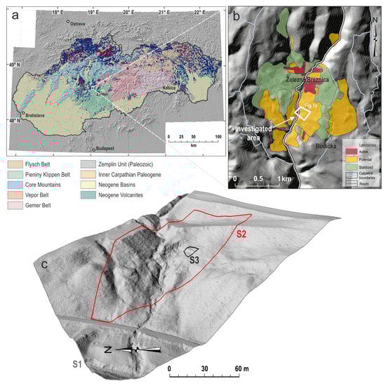
Figure 1.
(a) Location of the study area: Map of main geological units of Slovakia with distribution of slope failures (modified after [,,]). Active and stable slope failures are depicted by red and blue colors, respectively. The location of the study area is shown by a white polygon. (b) Shaded relief map of the investigated area near Železna Breznica village. Landslides registered in national database (modified after []) and the position of the investigated area are shown. (c) Detailed view on the studied slope. S1, S2, and S3 polygons are related to the light detection and ranging (LiDAR), remotely piloted aircraft system (RPAS), and close-range photogrammetry (CRP) survey technologies, respectively.
A map in Supplement 1 and a graph in Supplement 2 show that prevailing area of active slope failures derived from the national database [,] overlaps the areas of very low, low, and moderate landslide susceptibility in the European Landslide Susceptibility version 1 Map (ELSUS 1000 v1 Map) []. The source data in Figure 1 and Supplementary Materials S1 and S2 were downloaded from web map servers.
The investigated gully-related complex landslide is a relatively small landslide (1.7 ha) localized in the slope classified as a potential for slope failure [,]. During the field survey (2013 and 2017), we observed that some parts were active. We assumed that the landslide is the result of three interacting factors: Constant groundwater supply from deep slope deposits, occasional surface run-off flowing from the nearby wetland and from historical road which are both located above the landslide, and the state road undercutting the landslide’s slope at the bottom in its ground position.
The landslide spreads on forested medium slopes. Prevailing inclination is up to 30%, but locally, in the main landslide body, steep slopes (31–70%) and scarps appear. It consists of two main parts. The upper part was rotationally drifted and the extruded soil substrate and rocks blocked the water run-off from the slope. A shallow sink hole occurred here, and surface run-off was transformed to the groundwater. The highest positions of this part are at altitudes of 470 m asl. The lower part of the landslide has an altitude ranging from 409 to 465 m asl. West-east oriented gullies divide this lower part into several segments. The deepest gully is in the northern part and it reaches depths between 5–10 m. Other shallower gullies branch out mainly to the south.
3. Materials and Methods
The following assumptions supported the proposed procedure of the landslide geomorphological feature identification through different large scales in DEMs-derivatives:
- Landslides are traditionally delineated by the visual interpretation of aerial photographs and field surveys []. However, this survey brings a lot of subjectivity and it is time-consuming and expensive in terms of data and workload []. Small landslide features can be extracted from the surface models created from the airborne LiDAR data [].
- Terrain topography is assumed to be a useful indicator of a slope movement. The characterization of terrain topography is essential to detect landforms changes caused by a landslide activity. One way to distinguish different landforms is to describe the surface roughness of areas. This parameter refers to the variability in elevation within a defined radius, and therefore it is very sensitive to the selected scale []. The surface roughness is considered to be an important indicator to measure the target topographic features of landslides []. Surface roughness is one of the best indicators to differentiate between stable and active landslide areas []. However, calculation of the maximum curvature (kmax) can be a more sensitive and efficient method to recognize, extract, and delineate particular discrete landslide features that indicate their activity from high-resolution DEMs with sub-meter cell accuracy.
- Upper units can undergo fracturing and extension with subsequent disintegration, subsidence, and various type of movements []. These processes result in the formation of tension cracks, fractures, scarps, or tear-off landforms at the tops (heads) of landslide slopes. Those terrain features are commonly good indicators of failure initiation []. Therefore, the methodology proposed in the article aims to interpret and highlight these topographic structures.
- The use of detailed 3D information terrain surfaces allow the investigation of slope failures at different spatial and temporal scales, including the mapping of geomorphologic features and shape recognition that can also be used to track objects or slope failures []. There exists large diversity of variables that can be derived from DEMs, and, from this aspect, they remain underexploited [].
Data processing can be performed by open source or commercial software at reasonable costs []. Open source GIS alternatives (we used SAGA GIS, Quantum GIS and GRASS) provide many algorithms to process a variety of secondary terrain attributes and detailed elevation models-derived (DEM) variables. In any case, DEM-derived variables are scale-dependent and extent of their usability corresponds with a GIS expert’s knowledge and experiences []. Hierarchical multiscale geomorphometric analysis of landslide units and selected landslide features drawn from the various data sources allows recognition and classification of multiscale landslide components []. Geomorphological features of the studied landslide were examined at several large scales ranging from 1:1320 to 1:100.
3.1. Data Acquisition in the Field
Three survey technologies, Airborne Laser Scanning (LiDAR), Aerial Photogrammetry performed by remotely piloted aircraft system (RPAS), and SfM Close-range photogrammetry (SfM CRP) were applied on S1, S2, and S3 segments of the study area (Figure 1c). The field survey was carried out in Spring 2011 (LiDAR) and Spring 2017 (RPAS and SFM CRP). The basic characteristics of the landslide survey technologies are summarized in Table 1 (data modified after []). Ground control points (GCPs) were measured using a total station Topcon GPT 9003M and a geodetic dual-frequency Topcon Hiper SK GNSS receiver with the Internet-enabled Slovak permanent observation service providing real-time data corrections with accuracies ranging from 0.02 to 0.04 m.

Table 1.
Applied technologies in data acquisition during the field survey.
3.2. Data Processing in GIS Laboratory
3.2.1. Check Points Transformation, Applied GIS Software, Modules, and Tools
Using identical check points in digital models, point clouds were transformed into the national coordinate system JTSK (JTSK is the Coordinate System of Uniform Trigonometric Cadastral Network which is obligatory in the Slovak Republic) (position), while elevations were registered in Baltic vertical datum after their adjustment (Bpv). Derived products from point clouds were composited by rectifying their geometric distortions to generate one coordinate system. Subsequently, these products were analyzed and evaluated in various GIS applications.
The SfM CRP data were processed in Agisoft Photoscan licensed software (Agisoft LCC, St. Petersburg, Russia) [] using a workstation PC with Intel Core i7 processor, 32 GB of RAM and the NVIDIA Quadro 4000M graphic card. Processing options were set to “High” for both accuracy of photo alignment and quality of dense cloud generation. A description of the options is available in the Photoscan manual []. Detailed descriptions of the 3D reconstruction process in the Photoscan software are described in various studies [,,].
The LAStools application Rapidlasso GmbH (unlicensed version no. 180907), authorized by Martin Isenburg [], was applied for point clouds analyses and data processing of *.las/*.laz files. DEM raster files in ASCII format were produced from point clouds. We did not apply any smoothing operations for DEMs because observed terrains had dissimilar morphological structures, and estimations of smoothing iteration numbers or smoothing methods were rather experimental outside the scope of this article. Moreover, landform classifications have limitations requiring broader research (spurious tiny ridges or drainage networks occur, and drainage networks exhibit disconnectivity) []. We attempted to identify rugged terrain features, and any smoothing could hide this important though micro-scaled landforms. Comparable accuracy of all acquired datasets enabled us to set an identical resolution with grid cell size of 0.15 m for all DEMs. We consider this resolution to be sufficient because a gridded digital terrain model of 0.25 m cell size was applied in another similar work [] where the authors derived representative micro-scale landslide features. The QGIS2Threejs module was used for 3D model visualizations.
LiDAR point clouds were pre-processed by the provider, and any additional point cloud adjustment was not possible. Therefore, we used LAStools to create DEMs (las2dem) directly from the LiDAR data. The sequence of the following (basic) workflow steps characterizes point cloud processing for the RPAS and SfM CRP data (data processing workflow with detailed calculations is found in Supplementary Materials S3):
- The Lasnoise tool was used to exclude low noise points [class 7] because, in case of ground point derivation in further steps, it is recommended to leave out low noise points []. Clusters of low points occur frequently in image areas that were strongly shadowed, which was the case of the RPAS photographing of the landslide in the rugged terrain under dense forest canopy.
- The Lasground_new tool was used for bare-earth extraction; it classifies points into ground points (class = 2) and non-ground points (class = 1), and we computed the height of each point (without replacing -z) above the ground [] in cases of the RPAS and the SfM CRP data.
- The Lasheight_classify tool computes the height of each point above the ground and creates normalized point clouds in the selected height or interval of heights []. This tool was used for the processing of RPAS point clouds because photogrammetric scanning was done above a dense canopy of trees, locally, with a lower level of shrubs and where bare-earth was not visible. Therefore, we took into consideration all points from the ground within a interval from 0 m to 0.1 m.
The Las2dem tool computed a gridded DEM from ground-based point clouds or from point clouds with additional height parameters from *.laz files pre-processed in previous steps. The DEM was created with actual *.laz values, and the elevation parameter was set to 0.15 m.
Raster derivatives from LAStools were subsequently interpreted in the Quantum Geographic Information System 3.2.3. (QGIS) and in the System for Automated Geoscientific Analyses 2.3.2 (SAGA) (modules are explained below) using the coordinate system EPSG 5513 (data processing workflow with detailed calculations is in Supplementary Material S3).
- Module of Slope, Aspect, and Curvature: Terrain curvature is one of the most essential local morphometric parameters applied in landform analyses []. It is a curvature of a principal section with the highest value of curvature at a given point of the topographic surface []. Maximal curvature is scale-sensible and dependent on the location of cells within a raster grid because the odd number of cells in the square window such that the cells on the edges of a DEM remain unclassified [] and its values can be positive (convex landforms), negative (concave landforms), or zero (planar slopes).
- Module of Valley Depth and Basic Terrain Analysis: The valley depth is one of several non-local morphometric factors affecting the landslide susceptibility and it is calculated as the vertical distance to the base level of the channel network []. The threshold value for the ridge detection was set to 4 for the LiDAR DEM and the RPAS DEM. The threshold value for the ridge detection for the DEM created from the SfM CRP data was set to a value of 1. The tension threshold defined by the percentage of cell size was set to a default of 1 for all DEMs. Module of Basic Terrain Analysis was used for the calculations of topographic wetness index (TWI), which is a combined type of morphometric variable. TWI can be used to predict future landslide movements []. Higher values of the TWI represent drainage depressions, or deeper erosive landforms as hollows, ravines, gullies and lower values represent crests and ridges. TWI visualized a drainage network in the studied landslide area in Figure 2.
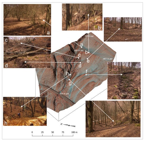 Figure 2. An active gully-related landslide system and micro-scale landforms features indicating its activity: (a) A collapsed sink; (b) terrain edge and exposed substrate and a bedrock; (c) a major scarp; (d) a minor scarp; (e) a terrain depression; (f) a spring with occasional water flow; (g) a ridge; and (h) a junction of gullies.
 - Module of Sky View Factor is not just an effective visualization method but also a powerful spatial analysis method with numerous applications []. A Sky View Factor is a solar morphometric variable interpreted in raster file—a shaded terrain model highlighting the brightness and contrast of landform discontinuities. It ranges from 1, for completely unobstructed surfaces (for example, horizontal surfaces, peaks and ridges), to 0, for completely obstructed surfaces []. We set up search radius to 100 m for the LiDAR and the RPAS data and to 5 m for the SfM CRP data.
The plugin CSMapMaker was applied for the landslide delineation and it is a licensed Python module that is released under the GNU Public License (GPL) Version 2 and authorized by Kosuke Asahi [].
3.2.2. Landslide Detection and Delineation in DEM Derivatives Generated from Point Clouds
The landslide was identified in DEMs using two approaches. Firstly, we applied the QGIS plugin CSMapMaker to make a CS (Curvature and Slope) topographic map from a DEM and to delineate landslide landforms. The CS topographic map displays the distribution of micro-relief in a mountainous area, and the author Kosuke Asahi suggested this tool for the evaluation of landslide susceptibility []. This plugin allows choosing of the parameters of the evaluated types of curvatures. The plugin was set up to calculate general curvature, and Gaussian filter parameters were set to 2 for standard deviation and to 10 for radius because these values showed the best results after the realization of several experiments. No other settings adjustment was possible in this module.
QGIS CSMapMaker produced similar terrain visualizations to a red relief image map (RRIM) [] which is a patented method especially developed to visualize the topographic detail acquired by LiDAR. It is a 3D visualization method [] for topography using the chroma of red color to show slope and the brightness of red color to show ridge-valley values calculated from DEM []. The CS topographic map comprised two rasters of slope, two rasters of general curvature which were all overlayed as 50% transparent rasters and smoothed DEM without transparency, and smoothed DEM. Valleys and ridges were depicted by bluish and reddish colors, respectively []. The chroma of red color was in the raster layers Slope 1 (grey shades) and Slope 2 (red shades). Slope was calculated in radians. General curvature 1 had the sequence of blue and red shades, and General curvature 2 had the sequence of blue shades. The DEM was smoothed with Gaussian filter and placed under the slope and curvature rasters. Further technical details are available in documentation for the CSMapMaker plugin [].
Secondly, we used a pixel-based method for the detection and delineation of basic landslide landforms. To identify terrain positions of the investigated landslide terrain, morphometric attributes like maximal curvature and sky view factor were analyzed. We multiplied the maximal curvature raster by the sky view factor raster. From the multiplied raster, we deducted the valley depth in order to eliminate sharp topographic features inside deep gullies and inside terrain depressions on the one side, and targeted landslide features indicating landslide activity were interpreted in the most general way as possible on the other side. The calculation of basic micro-scale landforms characterizing the complex gully-related landslide was done in a raster calculator (Supplementary Material S3).
A classification of raster into categories and the setup of thresholds is always terrain-dependent. The proposed classification was adopted particularly for the investigated landslide. The first it aimed to detect the entire landslide body from the surrounding terrain (sharp curved terrain edges or steps). Secondly, it aimed to generalize the variability and the complexity of micro-scale landforms of the studied landslide and to highlight sharp topographic features delineating particular parts of the complex gully system (sharp-crested ridges) and features indicating the landslide activity. The quantile classification assigns an equal pixel count for the classification, and no ‘empty’ and no ‘too many values’ classes exist. Therefore, widely different values can appear in the same class, or similar values can be presented in different classes. On the other hand, we considered the quantile classification to be ideal for ordinal data, i.e., for data ranking within categories such as, e.g., low, medium and high []. The final raster was divided into 5 categories to interpret only basic landforms, and classification of color symbology had 4 quantile breaks dividing raster into 5 discrete categories. The most negative values were assigned to the deepest concave landforms of the deepest slopes of gullies; less negative values were associated with slopes of upper parts of gullies or shallow concave landform terrain depressions or sink holes occurring locally and sporadically with occasional water flow. Values close to zero were assigned to gently curved concave, convex, or plane slopes located above the previous two categories. The highest values were assigned to the uppermost, ‘highest places upward’ (convex), and sharply-curved landforms.
The DEM of the investigated minor scarp was processed in a detailed scale of 1:100. The terrain raster was converted to a vector ESRI shape file where the minor scarp was delineated automatically.
4. Results
The landslide presented in the article is visualized as a 3D model in Figure 2. The model was constructed from the following overlaid raster files: DEM derived from LiDAR point clouds (read more in Material and Methods), topographic wetness index, and sky-view factor highlighting shades and lights of sharply-curved landforms. Major and minor scarps (Figure 2c,d) were considered as micro-scale landforms demonstrating the landslide activity (bare-rock with uncovered trees roots is visible in their tear-off part), and therefore we presented the detection and delineation of one minor scarp (Figure 2d) in our results.
Micro-scale landforms presented in Figure 3a,b outline the main boarders of the gully-related landslide area as well as its subdivision into several gullies, alternated with sharp-crested ridges. The contrast between the deepest parts of gullies or terrain depressions and the upward sharply-curved landform is self-evident (Figure 3b). From other aspects, sharply-curved convex landforms can be recognized as: (1) sharp-crested ridges oriented perpendicular to contour lines and dividing a complex gully system into several branches; (2) other sharp topographic feature oriented parallel to contour lines and delineating the entire landslide body from surrounding terrain in its upper older part; and (3) minor and major scarps, tension cracks and tear-off parts of the landslide or undulating terrain indicating the landslide activity. One minor scarp (it has a position of smaller red polygon in Figure 3a,b) was selected for a detailed survey by the SfM CRP method as we will show below. We considered this scarp to be an indicator of the recent landslide movement because fresh bare-rock and many uprooted trees appeared here, and many cracks in the soil substrate appeared in the scarp’s vicinity.
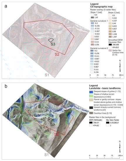
Figure 3.
Delineation of a gully related landslide system in a digital elevation model (DEM) generated from point clouds acquired by aerial laser scanning using the LiDAR technology applying the (a) CSMapMaker QGIS plugin and (b) Raster operation. The depth of valleys was deducted from multiplied raster files of maximal curvature and sky-view factor, and the output raster indicates basic landforms of the investigated landslide.
The usage of the RPAS technology for data collection appeared to be a useful tool for mapping the landslide shapes under certain conditions of terrain visibility for the RPAS camera. It means that RPAS technology was successfully applied in the forest with presence of many gaps in the forest canopy caused by the landslide activity which uprooted many trees. Thus, landforms were well visible for the RPAS camera. Data gaps appearing in “ground”-classified point clouds were eliminated by applying an additional parameter of “height” in LAStools, and both classifications were applied in the DEM creation (Supplementary Material S4). However, many data gaps remained in the digital model, and the missing data was mirrored, apparently, in derived raster and vector files (see, for instance, contour lines in Figure 4a). In areas where terrain was well visible of the RPAS camera, convex sharply-curved landforms were interpreted more precisely (Figure 4a,b) than it was in raster derivatives from LiDAR data (Figure 3b), mainly due to higher point cloud density.
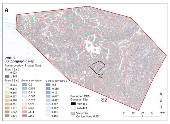
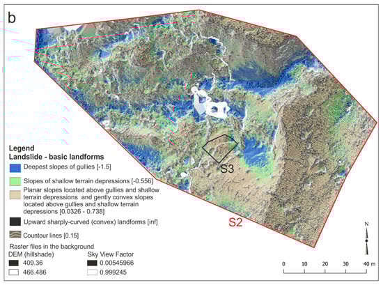
Figure 4.
Delineation of a gully related landslide system in a DEM generated from point clouds acquired by aerial laser scanning using the RPAS technology applying the (a) CSMapMaker QGIS plugin and (b) Raster operation. The depth of valleys was deducted from multiplied raster files of maximal curvature and sky-view factor, and the output raster indicates basic landforms of the investigated landslide.
CRP performed by the SfM method brought data of high quality and allowed visualization of micro-scale landforms in detail at a scale of 1:100. Thus, it would be easy to obtain relatively precise measurements regarding data accuracy of a particular technology and raster resolution applied for the DEM created from point clouds. While a steep tear-off slope of a minor scarp appears as an exact black color in the raster (Figure 5b), the CSMM plugin for the delineation of landslide landforms generated the tear-off slope as contrast of linear labeled colors demonstrating the steepest and the most rugged convex and concave landforms (Figure 5a).
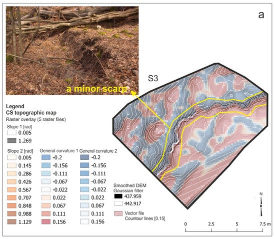
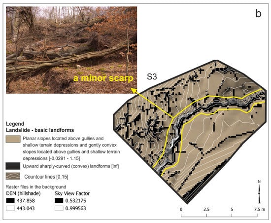
Figure 5.
Delineation of a minor scarp in a DEM generated from point clouds acquired by aerial laser scanning using the technique of close-range photogrammetry using ‘Structure-from-Motion’ method (SfM CRP) applying the (a) CSMapMaker QGIS plugin and (b) Raster operation. The depth of valleys was deducted from multiplied raster files of maximal curvature and sky-view factor, and the output raster indicates basic landforms of the investigated landslide.
We observed raster data mismatches between the LiDAR data and both the RPAS and the SfM CRP datasets. The minor scarp represented by upward sharply-curved landforms had a different shape in LiDAR-derived and RPSAS- and SfM CRP-derived data (Figure 6a). While the scarp’s shape in the raster derived from LiDAR was more linear, the minor scarp derived from both types of more recent data, RPAS and SfM CRP, had analogical S-shaped form (Figure 6b). Therefore, this mismatch is more likely a result of movements in the minor scarp area between years 2011 and 2017 than data inaccuracy.
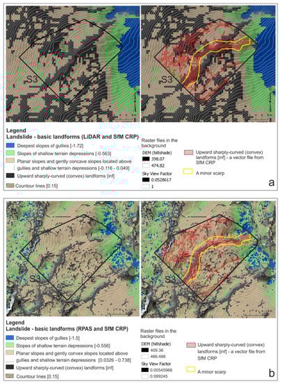
Figure 6.
Minor scarp documented in raster files visualizing landslide landforms derived from data gathered by (a) LiDAR (Spring 2011) and SfM CRP (Spring 2017) in red, and (b) RPAS and SfM CRP (Spring 2017) in red.
5. Discussion
The article presents partial results of the study focused on the large-scale survey of the landslide micro-topography. The proposed methodology has to be validated in other sites with different natural conditions and in broader areas at smaller scales to demonstrate its adequacy and in order to be enhanced and further developed. Our results follow the conclusions of the previous authors. [,,,,,,] that uncharted landslides can be discovered and recorded using costless technologies. Still, relatively expensive data from LiDAR can be regularly updated with datasets acquired from the aerial RPAS or from the terrestrial SfM CRP technologies. A terrestrial scanning is a costless and effective technique for supplementary mapping of deeply rugged, steep, and shaded areas under dense tree canopy where the LiDAR and the RPAS data have insufficient data density. Moreover, this technique can be used for the regular updating of the LiDAR data [].
Topographic derivative maps of DEMs allow detecting and classifying landslides, but not every landslide body is clearly recognizable from the surrounding terrain. Therefore, we developed a methodology for clear classification of sharp-edge-delineating micro-scale convex landforms, and local morphometric variables of maximal curvature was applied for this purpose. Convex sharply-curved landforms located in elevated positions of landslides slopes are good indicators of the initiation of slope failures. The presented method can thus be a valuable complementary method to other methods commonly used in mapping landslides and erosional landforms from digital terrain models, including TWI, topographic position index (TPI) [], or surface roughness []. The CSMM plugin, which produces CS topographic maps, suggested by the author Kosuke Asahi for the delineation of landslide features [] generated the tear-off slope of the minor scarp as a contrast of linearly labeled colors (dark grey and dark red) demonstrating the steepest slopes and the contact of the most rugged convex and concave landforms. However, this method did not allow direct automatic conversion of the minor scarp from the raster to the vector ESRI shapefile. Using the method suggested in our paper, basic landforms were classified into discrete classes and then automatically converted to an ESRI shapefile. The vector file can be further processed in different ways; for instance, the vector geometry can be smoothed and adopted for the further investigation of the landslide movement in the future.
The automatic or semi-automatic detection of landslides and their features from a very-high resolution LiDAR DEM using pixel-based approach is a challenging task, given that geomorphological features located at different locations in a landslide can indicate the same processes, but their contextual relations are not considered or considered marginally in this approach []. We partially solved this issue by the semi-automatic classification of upward sharply-curved micro-scale landforms with elevated positions in terrain that can potentially undergo fracturing and extension. These geomorphological features can be derived from the LiDAR and from the RPAS data. Furthermore, their real status can be verified or monitored in the field using the SfM CRP method or the Google Tango technology that was already tested for mapping of landslides under forest canopy [].
The required point cloud density is a relative parameter and varies according to the targeted interpretation scale of landslide’s features. Gross geomorphological features of landslides are detectable with the usage of a point density of 1.69 points m2 while micro-scale features require a point density more than 5.69 points m2 []. The authors recommend combining the interpretation of LiDAR-derived images with aerial photographs to get the best results in mountainous and densely vegetated areas. Technologies of LiDAR, RPAS, and CRP performed by the SfM method applied in this article brought much more dense point clouds (at least 9 points m2 in case of the LiDAR data). Relatively dense point clouds enabled the precise classification of basic landslide features and observation of micro-scale landforms, e.g., a minor scarp across different scales (Figure 7). The geodetic Topcon Hiper SK GNSS receiver provided data with accuracies ranging from 0.02 to 0.04 m. The LiDAR data can be used as a benchmark to solve the problem of insufficient control points. The error range of the RPAS data (positional error was 0.05 m and vertical error was 0.03 m) was not significantly different from those of the LiDAR (spatial error was 0.047 m) and the SfM CRP datasets (positional error was 0.02 m and vertical error was 0.007 m).
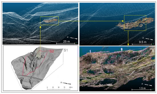
Figure 7.
The investigated minor scarp documented in merged point clouds from the LiDAR data (Spring 2011) and CRP SfM data (Spring 2017). Point clouds were merged in CloudCompare v2.9.1.
In general, we agree that aerial photogrammetry is not an entirely appropriate technique for mapping landslides in forested hilly regions [] mainly due to insufficient visibility of the surveyed terrain. Nevertheless, there exists a potential for the usage in a such environments. Regarding the factor of terrain visibility, timing of the aerial survey is very important. It shall be performed mainly during a period of vegetation dormancy when deciduous forests do not have tree canopy []. The authors documented that under optimal conditions, the root mean square coordinate errors (RMSE) of digital surface models derived from aerial photogrammetry ranged from 0.291 to 0.355 m. We performed the survey in Spring during the period of vegetation dormancy, and a scanning device had overall good visual contact with the ground and was very good, locally, in areas where the landslide was the most active and uprooted trees lay on the ground. Our results proved similar accuracies and data usability of both the RPAS and SfM CRP methods (Figure 6b). Considering the point cloud density (500 points m2) of the RPAS dataset, its positional (0.05 m) and vertical accuracy (0.03 m) was comparable with the dataset acquired from the SfM CRP method. The suggested RPAS aerial photogrammetry can be the optimal choice for investigations over small areas due to its advantages of portability, low costs, and speedy data processing [].
The high data quality allowed us to compare the LiDAR data of the minor scarp gathered in Spring 2011 with the RPAS and the SfM CRP data which were gathered in Spring 2017. Visible changes of the minor scarp shape in the DEM-derivatives (Figure 6a) could indicate landslide activity. The observation highlights the need for future monitoring of the study area and underlines the usability of the proposed method.
6. Conclusions
Public demands and the need to support decision-making processes with the visualization of alternative spatial resolutions forces geo-designers to introduce more-or-less digital and automated techniques into practice []. We analyzed and interpreted landslide data acquired by the light detection and ranging (LiDAR) technology, remotely piloted aircraft system (RPAS), and close-range photogrammetry (CRP) using ‘Structure-from-Motion’ (SfM) method. Results demonstrated the multiscale semi-automatic recognition of morphometric landslide features from high resolution DEM. Output DEMs-derivatives highlighted gross basic landslide landforms as well as micro-scale geomorphological features indicating the landslide activity (e.g., major and minor scarps, undulating terrain, etc.). The landslide characteristics can be computed through numerous methodologies. Nevertheless, at the beginning of the data acquisition and the subsequent processing, it is very important to specify the main landslide characteristics which are expected to be derived from point clouds. We have proven that existing data gaps or incomplete datasets can be easily filled with data from the SfM CRP method as confirmed in the results. Moreover, the proposed semi-automatic pixel-based method for the detection and delineation of the whole landslide body and its micro-scale landforms can be effectively applied for the mapping of landslides and erosional landforms from digital terrain models and thus extend the group of methods commonly used for this purpose.
Supplementary Materials
The following are available online at https://www.mdpi.com/2076-3263/9/3/117/s1. S1: The study area in Slovakia and its location in ELSUS (1000) map with categories of landslide susceptibility, modified after [] and the comparison with slope failures—landslides characterized in the national database of slope failures of the Slovak Republic, modified after [,]; S2: Categories of slope failures derived from the national database of the Slovak Republic, modified after [,] within categories of landslide susceptibility derived from the ELSUS (1000) map, modified after [] in the cadastral districts of Železná Breznica, Budička, and Tŕnie; S3: The LiDAR, RPAS, and SfM CRP data processing workflow; S4: (a) Data gaps in point clouds acquired by the RPAS technology. Point clouds were filtered with a ground points classification filter; Sky View Factor highlights terrain discontinuities and obstructions in digital model derived from ground classified point clouds with more data gaps; (b) Point clouds were filtered with a ground points classification filter using the parameter from the height classification (drop points of the ground within interval from 0 to 0.1 m); Sky View Factor highlights terrain discontinuities and obstructions in digital model derived from ground classified point clouds with less data gaps.
Author Contributions
Conceptualization, F.C. and M.S.; methodology, M.S., F.C., and J.T.; software, J.T., M.S., and M.M.; validation, M.S.; formal analysis, M.S.; investigation, J.T. and F.C.; resources, M.S. and R.P.; data curation, J.T., M.M., and F.C.; writing—original draft preparation, M.S.; writing—review and editing, R.P.; visualization, M.S.; supervision, F.C.; project administration, J.T.; funding acquisition, F.C.
Funding
This research was funded by Vedecká Grantová Agentúra MŠVVaŠ SR a SAV grant number 1/0868/18 (Innovative techniques for mapping of anthropogenic and natural landforms applicable in survey of landscape status).
Acknowledgments
The LiDAR data were acquired during the recent project “Centre of excellence for decision support in forest and country, ITMS: 26220120069.” The authors thank the collaborators Daniel Tunák and Šimon Saloň who carried out an essential part of the fieldwork.
Conflicts of Interest
The authors declare no conflict of interest. The founding sponsors had no role in the design of the study; in the collection, analyses, or interpretation of data; in the writing of the manuscript, and in the decision to publish the results.
References
- Mora, O.E.; Liu, J.K.; Lenzano, M.G.; Toth, C.K.; Grejner-Brzezinska, D.A. Small Landslide Susceptibility and Hazard Assessment Based on Airborne Lidar Data. Photogramm. Eng. Remote Sens. 2015, 81, 239–247. [Google Scholar] [CrossRef]
- Huang, H.; Song, K.; Yi, W.; Long, J.; Liu, Q.; Zhang, G. Use of multi-source remote sensing images to describe the sudden Shanshucao landslide in the Three Gorges Reservoir, China. Bull. Eng. Geol. Environ. 2018, 1–20. [Google Scholar] [CrossRef]
- Del Soldato, M.; Riquelme, A.; Bianchini, S.; Tomàs, R.; Di Martire, D.; De Vita, P.; Moretti, S.; Calcaterra, D. Multisource data integration to investigate one century of evolution for the Agnone landslide (Molise, southern Italy). Landslides 2018, 15, 1–16. [Google Scholar] [CrossRef]
- Mora, O.E.; Lenzano, M.G.; Toth, C.K.; Grejner-Brzezinska, D.A.; Fayne, J.V. Landslide Change Detection Based on Multi-Temporal Airborne LiDAR-Derived DEMs. Geosciences 2018, 8, 23. [Google Scholar] [CrossRef]
- Abellan, A.; Derron, M.-H.; Jaboyedoff, M. “Use of 3D Point Clouds in Geohazards” Special Issue: Current Challenges and Future Trends. Remote Sens. 2016, 8, 130. [Google Scholar] [CrossRef]
- Peternel, T.; Kmelj, Š.; Oštir, K.; Komac, M. Monitoring the Potoška planina landslide (NW Slovenia) using UAV photogrammetry and tachymetric measurements. Landslides 2017, 14, 395–406. [Google Scholar] [CrossRef]
- Prokešová, R.; Kardoš, M.; Tábořík, P.; Medveďová, A.; Stacke, V.; Chudý, F. Kinematic behaviour of a large earthflow defined by surface displacement monitoring, DEM differencing, and ERT imaging. Geomorphology 2014, 224, 86–101. [Google Scholar] [CrossRef]
- Chudý, F.; Slámová, M.; Tomaštík, J.; Tunák, D.; Kardoš, M.; Saloň, Š. The application of civic technologies in a field survey of landslides. Land Degrad. Dev. 2018, 29, 1858–1870. [Google Scholar] [CrossRef]
- Razak, K.A.; Straatsma, M.W.; van Westen, C.J.; Malet, J.P.; de Jong, S.M. Airborne laser scanning of forested landslides characterization: Terrain model quality and visualization. Geomorphology 2011, 126, 186–200. [Google Scholar] [CrossRef]
- Pirasteh, S.; Li, J. Landslides investigations from geoinformatics perspective: Quality, challenges, and recommendations. Geomatics. Geomat. Nat. Hazards Risk 2016, 1–18. [Google Scholar] [CrossRef]
- Godone, D.; Giordan, D.; Baldo, M. Rapid mapping application of vegetated terraces based on high resolution airborne LiDAR. Geomat. Nat. Hazards Risk 2018, 9, 970–985. [Google Scholar] [CrossRef]
- Kaiser, A.; Neugirg, F.; Rock, G.; Müller, C.; Haas, F.; Ries, J.; Schmidt, J. Small-Scale Surface Reconstruction and Volume Calculation of Soil Erosion in Complex Moroccan Gully Morphology Using Structure from Motion. Remote Sens. 2014, 6, 7050–7080. [Google Scholar] [CrossRef]
- Medjkane, M.; Maquaire, O.; Costa, S.; Roulland, T.; Letortu, P.; Fauchard, C.; Antoine, R.; Davidson, R. High-resolution monitoring of complex coastal morphology changes: Cross-efficiency of SfM and TLS-based survey (Vaches-Noires cliffs, Normandy, France). Landslides 2018, 15, 1097–1108. [Google Scholar] [CrossRef]
- Sturdivant, E.J.; Lentz, E.E.; Thieler, E.R.; Farris, A.S.; Weber, K.M.; Remsen, D.P.; Miner, S.; Henderson, R.E. UAS-SfM for Coastal Research: Geomorphic Feature Extraction and Land Cover Classification from High-Resolution Elevation and Optical Imagery. Remote Sens. 2017, 9, 1020. [Google Scholar] [CrossRef]
- Stumpf, A.; Malet, J.P.; Allemand, P.; Pierrot-Deseilligny, M.; Skupinski, G. Groundbased multi-view photogrammetry for the monitoring of landslide deformation and erosion. Geomorphology 2015, 231, 130–145. [Google Scholar] [CrossRef]
- Westoby, M.J.; Brasington, J.; Glassera, N.F.; Hambreya, M.J.; Reynolds, J.M. ‘Structure-from-Motion’ photogrammetry: A low-cost, effective tool for geoscience applications. Geomorphology 2012, 179, 300–314. [Google Scholar] [CrossRef]
- Chudy, F.; Sadibol, J.; Slamova, M.; Belacek, B.; Pažinova, N.; Beljak, J. Identification of Historic Roads in the Forest Landscape by Modern Contactless Methods of Large-Scale Mapping. In Proceedings of the GeoConference on Informatics, Geoinformatics and Remote Sensing, Albena, Bulgary, 17–26 June 2014; Volume 3, pp. 183–190. [Google Scholar] [CrossRef]
- Roberto, R.; Lima, J.P.; Araújo, T.; Teichrieb, V. Evaluation of Motion Tracking and Depth Sensing Accuracy of the Tango Tablet. In Proceedings of the 2016 IEEE International Symposium on Mixed and Augmented Reality (ISMAR-Adjunct), Merida, Yucatan, Mexico, 19–23 September 2016; Veas, E., Langlotz, T., Martinez-Carranza, J., Eds.; The Institute of Electrical and Electronics Engineers, Inc.: Danvers, MA, USA, 2016; pp. 231–234, ISBN 978-1-5090-3740-7. [Google Scholar] [CrossRef]
- Tomaštík, J.; Saloň, Š.; Tunák, D.; Chudý, F.; Kardoš, M. Tango in forests—An initial experience of the use of the new Google technology in connection with forest inventory tasks. Comput. Electron. Agric. 2017, 141, 109–117. [Google Scholar] [CrossRef]
- Giordan, D.; Manconi, A.; Tannant, D.D.; Allasia, P. UAV: Low-cost remote sensing for high-resolution investigation of landslides. In Proceedings of the 2015 IEEE International Geoscience and Remote Sensing Symposium (IGARSS), Milan, Italy, 26–31 July 2015; The Institute of Electrical and Electronics Engineers, Inc.: Danvers, MA, USA, 2015; pp. 5344–5347, ISBN 978-1-4799-7929-5. [Google Scholar] [CrossRef]
- Jiang, L.; Ling, D.; Zhao, M.; Wang, C.; Liang, O.; Liu, K. Effective Identification of Terrain Positions from Gridded DEM Data Using Multimodal Classification Integration. ISPRS Int. Geo-Inf. 2018, 7, 443. [Google Scholar] [CrossRef]
- Newman, D.R.; Lindsay, J.B.; Cockburn, J.M.H. Evaluating metrics of local topographic position for multiscale geomorphometric analysis. Geomorphology 2018, 312, 40–50. [Google Scholar] [CrossRef]
- Hou, W.; Lu, X.; Wu, P.; Xue, A.; Li, L. An Integrated Approach for Monitoring and Information Management of the Guanling Landslide (China). ISPRS Int. J. Geo-Inf. 2017, 6, 79. [Google Scholar] [CrossRef]
- Bednarik, M.; Liščák, P. Landslide susceptibility assessment in: Slovakia. Mineralia Slovaca 2010, 42, 193–204. [Google Scholar]
- Vass, D. Regional-Geological Division of the Slovak Republic, 1:500,000 [online]. Available online: http://apl.geology.sk/temapy (accessed on 12 October 2018). (In Slovak).
- Maglay, J.; Pristaš, J.; Kučera, M.; Ábelová, M.; Fritzman, R.; Vlachovič, J.; Bystrická, G.; State Geological Institute of Dionyz Stur, Slovakia; Ministry of the Environment of the Slovak Republic; Geodesy, Cartography and Cadaster Office of the Slovak Republic. 2009: Quaternary Geological Map of the Slovak Republic, 1:500,000 [online]. Available online: http://apl.geology.sk/temapy/ (accessed on 12 October 2018). (In Slovak)
- Šimeková, J.; Martinčeková, T.; Abrahám, P.; Gejdoš, T.; Grenčíková, A.; Grman, D.; Hrašna, M.; Jadroň, D.; Záthurecký, A.; Kotrčová, E.; et al. The Atlas of the Slope Stability Maps of the Slovak Republic at a Scale 1:50,000; INGEO-IGHP: Žilina, Slovakia, 2006; 155p. (In Slovak) [Google Scholar]
- Slope Failures of the Slovak Republic. Available online: http://apl.geology.sk/geofond/zosuvy// (accessed on 12 October 2018). (In Slovak).
- Günther, A.; Hervás, J.; Van Den Eeckhaut, M.; Malet, J.P.; Reichenbach, P. Synoptic pan-European landslide susceptibility assessment: The ELSUS 1000 v1 map. In Landslide Science for a Safer Geoenvironment; Sassa, K., Canuti, P., Yin, Y., Eds.; Springer: Cham, Switzerland, 2014; pp. 117–122. [Google Scholar] [CrossRef]
- Długosz, M. Digital Terrain Model (DTM) as a Tool for Landslide Investigation in The Polish Carpathians. Studia Geomorphologica Carpatho-Balcanica 2012, XLVI, 5–23. [Google Scholar] [CrossRef]
- Hölbling, D.; Füreder, P.; Antolini, F.; Cigna, F.; Casagli, N.; Lang, S. A Semi-Automated Object-Based Approach for Landslide Detection Validated by Persistent Scatterer Interferometry Measures and Landslide Inventories. Remote Sens. 2012, 4, 1310–1336. [Google Scholar] [CrossRef]
- Schillaci, C.; Braun, A.; Kropáček, J. Terrain analysis and landform recognition. In Geomorphological Techniques; British Society for Geomorphology: London, UK, 2015; Chapters 2.4.2; pp. 1–18. ISSN 2047-0371. [Google Scholar]
- Berti, M.; Corsini, A.; Daehne, A. Comparative analysis of surface roughness algorithms for the identification of active landslides. Geomorphology 2013, 182, 1–18. [Google Scholar] [CrossRef]
- Varnes, D.J. Slope Movement Types and Processes. In Landslides: Analysis and Control, National Research Council, Washington DC, Transportation Research Board, Special Report 176; Schuster, R.L., Krizek, R.J., Eds.; National Academy Press: Washington, DC, USA, 1978; pp. 11–33. [Google Scholar]
- Highland, L.M.; Bobrwosky, P. The Landslide Handbook—A Guide to Understanding Landslides; The U.S. Geological Survey: Reston, VA, USA, 2008; p. 11. ISBN 9781411322264.
- Leempoel, K.; Parisod, C.; Geiser, C.; Daprà, L.; Vittoz, P.; Joost, S. Very high-resolution digital elevation models: Are multi-scale derived variables ecologically relevant? Methods Ecol. Evol. 2015, 6, 1373–1383. [Google Scholar] [CrossRef]
- AgiSoft PhotoScan Professional. Software and Software Manual 2018. Available online: http://www.agisoft.com (accessed on 10 December 2018).
- Del Soldato, M.; Riquelme, A.; Tomás, R.; De Vita, P.; Moretti, S. Application of Structure from Motion photogrammetry to multi-temporal geomorphological analyses: Case studies from Italy and Spain. Geogr. Fis. Dinam. Quat. 2018, 41, 51–66. [Google Scholar] [CrossRef]
- Riquelme, A.; Del Soldato, M.; Tomás, R.; Cano, M.; Bordehore, J.L.; Morettic, S. Digital landform reconstruction using old and recent open access digital aerial photos. Geomorphology 2019, 329, 206–223. [Google Scholar] [CrossRef]
- Rapidlasso GmbH, Lasnoise. Available online: https://rapidlasso.com/lastools/ (accessed on 15 November 2018).
- Rana, S. Use of Plan Curvature Variations for the Identification of Ridges and Channels on DEM. In Progress in Spatial Data Handling: 12th International Symposium on Spatial Data Handling; Riedl, A., Kainz, W., Elmes, A.G., Eds.; Springer: Berlin/Heidelberg, Germany, 2006; pp. 789–804. ISBN 978-3-540-35588-5. [Google Scholar] [CrossRef]
- Krebs, P.; Stocker, M.; Pezzatti, G.B.; Conedera, M. An alternative approach to transverse and profile terrain curvature. Int. J. Geogr. Inf. Sci. 2015, 29, 643–666. [Google Scholar] [CrossRef]
- Curvature, Earth and Planetary Sciences, Science Direct. Available online: https://www.sciencedirect.com/topics/earth-and-planetary-sciences/curvature (accessed on 5 October 2018).
- Lee, S.; Lee, M.J.; Lee, S. Spatial prediction of urban landslide susceptibility based on topographic factors using boosted trees. Environ. Earth Sci. 2018, 77, 656. [Google Scholar] [CrossRef]
- Ylmaz, I. Landslide susceptibility mapping using frequency ratio, logistic regression, artificial neural networks and their comparison: A case study from Kat landslides (Tokat—Turkey). Comput. Geosci. 2009, 35, 1125–1138. [Google Scholar] [CrossRef]
- Zakšek, K.; Oštir, Ž.; Kokalj, O. Sky-View Factor as a Relief Visualization Technique. Remote Sens. 2011, 3, 398–415. [Google Scholar] [CrossRef]
- Harris, A.; Baird, A.J. Microtopographic Drivers of Vegetation Patterning in Blanket Peatlands Recovering from Erosion. Ecosystems 2018, 1–20. [Google Scholar] [CrossRef]
- QGIS Python Plugins Repository, Plugins by Kosuke ASAHI. Available online: https://plugins.qgis.org/plugins/author/Kosuke%20ASAHI/ (accessed on 14 November 2018).
- Kaneda, H.; Chiba, T. Stereopaired Morphometric Protection Index Red Relief Image Maps (Stereo MPI-RRIMs): Effective Visualization of High-Resolution Digital Elevation Models for Interpreting and Mapping Small Tectonic Geomorphic Features. Bull. Seismol. Soc. Am. 2019, 108. [Google Scholar] [CrossRef]
- Red Relief Image Map. Available online: https://www.rrim.jp/en/patent/ (accessed on 22 January 2019).
- Chiba, T.; Kaneta, S.; Suzuki, Y. Red Relief Image Map, New Visualization Method for Three Dimensional Data. Int. Arch. Photogramm. Remote Sens. Spat. Inf. Sci. 2008, 37, 1071–1076. [Google Scholar]
- CSMapMaker. Available online: https://github.com/waigania13/CSMapMaker (accessed on 31 January 2019).
- GISGeography. Available online: https://gisgeography.com/quantile-classification-gis/ (accessed on 12 December 2018).
- Holata, L.; Plzák, J.; Světlík, R.; Fonte, J. Integration of Low-Resolution ALS and Ground-Based SfM Photogrammetry Data. A Cost-Effective Approach Providing an ‘Enhanced 3D Model’ of the Hound Tor Archaeological Landscapes (Dartmoor, South-West England). Remote Sens. 2018, 10, 1357. [Google Scholar] [CrossRef]
- Różycka, M.; Migoń, P.; Michniewicz, A. Topographic Wetness Index and Terrain Ruggedness Index in geomorphic characterisation of landslide terrains, on examples from the Sudetes, SW Poland. Z. Geomorphol. 2017, 61, 61–80. [Google Scholar] [CrossRef]
- Korzeniowska, K.; Korup, O. Mapping gullies using terrain surface roughness. In Proceedings of the 19th AGILE International Conference on Geographic Information Science (AGILE 2016), Helsinki, Finland, 14–17 June 2016; Sarjakoski, T., Yasmina, M., Sarjakoski, S., Sarjakoski, T., Eds.; The Association of Geographic Information Laboratories for Europe (AGILE): Helsinky, Finland, 2016; p. 5, ISBN 978-3-319-33782-1. [Google Scholar]
- Guzzetti, F.; Mondini, A.C.; Cardinali, M.; Fiorucci, F.; Santangelo, M.; Chang, K.T. Landslide inventory maps: New tools for and old problem. Earth-Sci. Rev. 2012, 112, 42–66. [Google Scholar] [CrossRef]
- Van den Eeckhaut, E.; Poesen, J.; Verstraeten, G.; Vanacker, V.; Nyssen, J.; Moeyersons, J.; van Beek, L.P.H.; Vandekerckhove, L. Use of LIDAR-derived images for mapping old landslides under forest. Earth Surf. Proc. Land 2006, 32, 754–769. [Google Scholar] [CrossRef]
- Hsieh, Y.-C.; Chan, Y.-C.; Hu, J.-C. Digital Elevation Model Differencing and Error Estimation from Multiple Sources: A Case Study from the Meiyuan Shan Landslide in Taiwan. Remote Sens. 2016, 8, 199. [Google Scholar] [CrossRef]
- Wilson, M.W. Paper on the criticality of mapping practices: Geodesign as critical GIS? Landsc. Urban Plan. 2015, 142, 226–234. [Google Scholar] [CrossRef]
© 2019 by the authors. Licensee MDPI, Basel, Switzerland. This article is an open access article distributed under the terms and conditions of the Creative Commons Attribution (CC BY) license (http://creativecommons.org/licenses/by/4.0/).