A Quantitative Evaluation of Hyperpycnal Flow Occurrence in a Temperate Coastal Zone: The Example of the Salerno Gulf (Southern Italy)

Abstract

The inner continental shelf is regarded as a repository of hyperpycnal flow (HF) deposits the analysis of which may contribute to hydrogeological risk assessment in coastal areas. In line with the source to sink paradigm, we examined the dynamics of the coastal watersheds facing the Salerno Gulf (Southern Tyrrhenian Sea) in generating hyperpycnal flows and investigated the shallow marine sediment record to verify their possible occurrence in the recent past. Thus, the morphometric properties (hypsometric integral, hypsometric skewness, hypsometric kurtosis, density skewness and density kurtosis) of the watersheds together with the potential rivers’ discharge and sediment concentration, calculated by applying altitude- and extent -based experimental relations, allowed to detect the rivers that were prone to producing HFs. In the shallow marine environment record of the last 2 kyr, anomalous sedimentation, possibly linked to HF events, was identified by comparing the sand-mud ratio (S/M) down-core —at three sites off the main river mouths — to the expected S/M calculated by applying the relation governing the present-day distribution of sand at the seabed in the Salerno Gulf. A return period of major HF events ≤ 0.1 kyr can be inferred for rivers which fall into the category “dirty rivers”. In these cases, the watersheds have a hypsometric index ranging between 0.2 and 0.3, coastal plains not exceeding 30% of the entire catchment area and a maximum topographic height ≥1000 m. A return period of about 0.3 kyr has been inferred for the “moderately dirty rivers”. In these other cases, about 50% of the watersheds develop into a low gradient coastal plain and have a hypsometric index ranging between 0.09 and 0.2. The observations on land and offshore have been complemented to reach a more comprehensive vision of the coastal area dynamics. The method here proposed corroborates the effectiveness of the source to sink approach and is applicable to analogous sediment records in temperate continental shelves which encompass the last 3 kyr, a time interval in which the oscillations of relative sea level can be overlooked.

1. Introduction

Floods are a common occurrence in Italy. Between 1279 and 2002, about 837 flooding events out of 1019 caused fatalities [1]. These events included sudden inundations caused by failure of levees and dams, inundations of major rivers as well as flash floods along torrents and minor streams. Between 1400 and 2002, the high magnitude of flood events was responsible for the highest number of fatalities in Emilia Romagna, Sicilia, Lazio and Lombardia regions while the density of fatal floods was the highest in Liguria, Campania and Friuli-Venezia Giulia regions [1].

Vennari et al. [2] analyzed the flood events occurred in the Campania Region, and pointed out that about 10% of them had been due to landslides, 25% to inundation events, 50% to overflows of torrential streams, while 9% to combined or undefined causes.

Floods events are referred to as flash floods when the rise of river level occurs during rainfall or within a few hours from the meteoric event [3]. They occur largely within small catchments, where the hydrological response time of the watershed is short [2,4,5], in hot arid environments [6,7] or in the small catchments of the Mediterranean region [8,9], characterized by dry summers and autumnal high-intensity rainfall events [5].

The Campania Region has been frequently affected by flash floods [10,11,12,13,14,15,16,17] that have drained into inland outlets, forming fans or well-defined foothills [16], or into coastal outlets, creating delta fans, that often result to be ephemeral [10,11]. The latter events can trigger hyperpycnal flows (hereafter HF), defined by Mulder and Syvitski [18], as “a negatively buoyant plume that flows along the basin floor due to plume density in excess of ambient density of the standing water-body, as the result of the sediment load that it carries”. HFs may occur episodically in small catchments up to a few hundred square kilometers wide, when rivers increase their competence within a few hours or even less from the rainfall event [6]. These conditions typify many mountainous watersheds close to the coast in the Mediterranean region [8]. The rivers most prone to generate HFs are the “dirty rivers”, characterized by an average suspended sediment concentration higher than 10 kg m⁻³ and low annual discharge [18].

The present paper focuses on the capability of small (≤10³ km²) mountainous rivers flowing in the Tyrrhenian Sea to generate HFs by using a Geographical Information System-based methodology which merges the results of experimental relations, mainly based on the morphological data of river basins, with the study of the deposits genetically linked to these events (HFD) in the shallow marine sediment record. We tested this methodology on the Bonea, Picentino, Tusciano, Asa, Sele and Solofrone river catchment areas (hereafter, SGCs), bordering the Salerno Gulf (Southern Italy), (Figure 1), the extent of which varies over three orders of magnitude (Sele 3400 km², Picentino, Tusciano and Solofrone between 100–230 km²; Bonea and Asa ≤ 32 km²), while the maximum relief varies between 400 and 2000 m a.s.l..

In the study area, of the 48 alluvial events recorded between 1580 and 1996 those that occurred in the years 1581, 1773, 1899, 1910, 1924, 1954, can be classified as catastrophic by their duration, amount of rainfall, number of consequent geological events (landslides, inundation, denudation of slopes), the extent of involved areas and the consequences on the population and urban environment [19,20]. In particular, the intense rainfall occurred on the October 25th, 1954 favored the mass movements of the sedimentary cover of steep slopes and the releasing of large amounts of material into the stream that formed an ephemeral delta [20,21]. In 1773, the same area was affected by extensive inundation, landslides and diffuse shoreline progradation (400–450 m) that caused severe damage to the infrastructures and about 400 fatalities [22].

In accordance with the empirical relation proposed by Milliman and Syvitski [23], and modified by Mulder and Syvitski [18], the watershed extent, the maximum relief area, the average river discharge and the river flood discharge were used to assess the potential capability of the SGCs to produce HFs. Moreover, to reveal the different behaviors of the SGCs in producing HFs, we calculated the hypsometric index and hypsometric parameters (hypsometric skew, hypsometric kurtosis, density skew, density kurtosis) to assess the watershed evolutionary status, the zones exposed to erosion, the presence of sudden drop height and their distance from the river outlet. We also calculated the Melton Ratio to identify the dominant sediment-transport processes in the SGCs [24].

The study of the deposits genetically linked to the HFs in the shallow marine sediment record is still a sensitive issue. Recent field observations and lab-scaled tests have reported that high-competent plunging flows, often triggered by major flash-floods, may carry fine to medium sand as a suspended load in turbulent regimes and a minor fraction of coarse sand and gravel as a bedload component [9,18,25,26]. In hyper-arid environments, up to 8% of the suspended material during a HF event may be sand, sized between 63 mµ and 2000 mµ [6]. The deposition of sandy event beds on the inner shelf is a function of the magnitude (instantaneous discharges and flow velocities) and time-duration of the flood event [6,26]. The sand tends to settle and eventually be buried while the mud component tends to be removed through time and dispersed at higher depth [27]. The preservation of the HF deposit largely depends on several factors such as: (i) the deposition depth, (ii) the percentage of sand versus mud, (iii) the burial rate, (iv) the bioturbation rate. It has also been observed that a post-depositional reworking in shallow waters may favor the dispersal of the mud component at depth and the consequent selective concentration of the coarse fraction which remains unaffected [27,28].

Despite the lively ongoing debate on the possibility that a HF would directly feed the slope channel/basin fan systems [8,25,29,30], there is a general consent that sediment lobes fed by episodic riverine HF can form in the inner shelf, below the storm wave base [31]. The fine-medium sand component in the resultant hyperpycnites may be relevant where the sourcing areas are mountainous catchments leaning against the coast, with reduced or almost absent alluvial plains [6,26]. The deposits consist of composite beds with longitudinally and laterally changing facies and with an important fraction of coarse sized grains (500 µm > x > 63 µm) and organic matter, ranging from inversely graded units overlain by a normally graded sequence, to massive units (resulting from steady conditions). The coarsening upward-fining upward transition marks the coarser fraction in the deposits and corresponds approximately to the peak of the flood and to the maximum discharge at the river mouth [6,32]. The inversely graded unit may be partly or totally eroded before deposition of the normally graded unit in the proximal settings depending on the shape of the flood hydrograph. The peak flood conditions thus may generate an intrasequence erosional contact. The upper and lower units may contain thin horizontal parallel laminations, cross bedding but also climbing ripples, or present no particular structure at all. The contact between the two units can be erosive sharp or gradational [6,33]. In the case of a natural river damming during a flood and successive dam draining, two sequences might stack: at the base a mass flow deposit contemporaneous with the damming and at the top sequence a classical hyperpycnite [6].

In view of the above and considering that small-sized coastal watersheds of mountainous rivers are likely to deposit fine to medium sandy-grained sediment directly offshore on the continental shelves [6,18,31] the grain size of twenty-two seabed samples and three marine sediment cores were examined to identify possible event beds in the sediment record. At this aim, we defined a numerical/statistical procedure to reinforce (or reject) the outcomes of the geomorphological analysis of the catchments on land. The quantitative procedure here proposed includes:

• the definition of the “normal” sand/mud ratio at the seabed in function of depth, by assessing a regression curve valid for the studied area—in this case in the Salerno Gulf—and based on the measurements of the sand/mud content in the grabs and in the uppermost levels of box-core;
• the identification of the horizons in the sediment record whose sand/mud ratio is higher than expected by the regression curve.

Since the occurrence of hyperpycnites in the sedimentary archives of sink areas is related to flood frequency and magnitude, their settlement should vary with relative sea level oscillations and climate changes [6]. The analyzed stratigraphic record spans back to no more than the last 2 ky, a time interval in which these variations can be overlooked. In the study area in fact, the post-Roman age has recorded high stand conditions, with normal regression of the coastline [34], a net sediment aggradation in the shallow marine environment (below the closure depth), a high sediment yield [35] and only a slight eustatic rise of sea level (+ 0.13 ± 0.09 m, [36]). This investigation was performed to analyze the functionality of small catchments and shallow marine environments as a whole system, according to the source-to-sink paradigm [37,38].

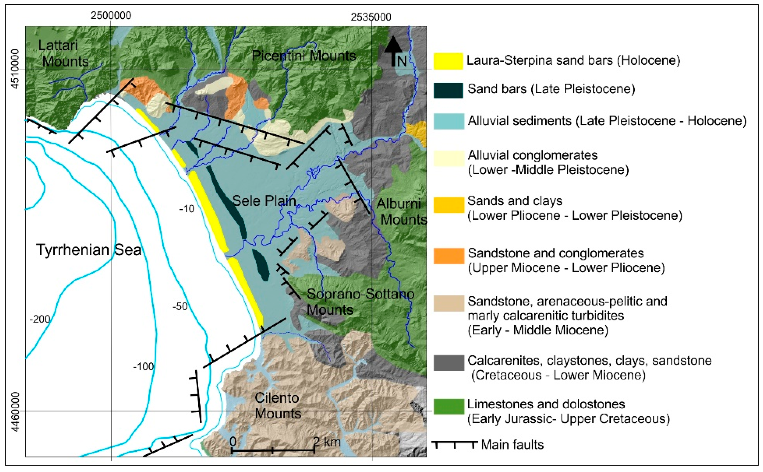
2. Geological and Morphological Settings

The Sele coastal plain occupies the inner portion of a structural depression trending WSW-ENE bounded by NE-SW normal faults and filled by about 3000 m of Plio-Plistocene sediments. Its origin is linked to the opening of the Marsili basin in the south-eastern sector of the Tyrrhenian Sea [39,40], a back-arc basin associated with the western subduction of the African Plate under the European Plate [41,42] and was coeval to the SE migration of the Calabrian subduction front [43].

The Sele Plain is bordered by the Picentini, Alburni and Soprano-Sottano mountains, made up of Meso-Cenozoic dolomite and limestone, blanketed by pyroclastic fall in many places, and subordinately pelitic and arenaceous deposits [44,45].

The inner most portion of this plain is characterized by hills up to 400 m high, formed by uplifted alluvial fans, representing the Early Pleistocene portion of the infill [46] and by epiclastic, alluvial, fluvial, lacustrine, lagoonal and marine deposits, Middle Pleistocene-Holocene in age [46,47] (Figure 2).

In the beginning of the Middle Pleistocene, the geomorphology of the plain was re-shaped by normal and transtensional faults. Part of the plain area carrying Early Pleistocene fanglomerates was uplifted, while a large part of the plain continued to subside. The latter accommodates some hundreds of coarse-grained sediments of fluvial origin, grey and blue clays of lagoonal systems, marine coastal sands and dunes, which, in the uppermost part of the succession, give evidence of several regression-transgression phases, tentatively framed between the OIS 9 and 5.5 [48,49]. Between 130 and 70 ka BP, three orders of beach-dune ridges formed and interfingered with lagoon and fluvio-paludal deposits [50].

The Late Pleistocene-Holocene transgression drove the palaeo-shoreline and the coastal system to transgress. Several relics of infralittoral prograding wedges have been found offshore below the maximum flooding surface [51] and relict shores, located inland about 1.5 km from the present-day coastline (Laura palaeoridge), document the maximum retrogradation stage of the barrier-lagoon coastal system, the age of which is approximatively, 5.5 ky BP [52]. Since then, the shoreline has prograded again and the barrier-lagoon system has migrated seaward, reaching the present position. A relict dune system subparallel to the present-day coastline can be linked to these phases which allowed the formation of the pre-2.5 ky Sterpina I ridge and then the syn-AD 79 Sterpina II ridge [34]. Coeval to this last renewed phase of normal regression are the infralittoral prograding wedges which lie offshore above the 79 AD Vesuvian pumice lapilli deposit, and feature an offlap break as deep as 25 m [51].

The continental shelf in the Salerno Gulf is about 9–20 km wide and bounded seawards by a sharp shelf break that is 120 m deep in the northern sector and 180 m deep in the southern sector [35]. The shelf break is located at a distance of 2–12 km from the coast in the northern sector, while southward it is 15–25 km distant from the coast. Such a pattern is due to the presence of a complex fault system that controls the shelf break position and the shelf slope morphology. Off the Sele River mouth, it has a width of 13 km and the shelf break is at a depth of 150 m (Figure 2). The thickness of the post 5 kyr marine sediment at the −25 m isobath is about 12 m off the Bonea River, 6 m off the Picentino and Asa rivers, 5 m off the Tusciano River, 9 m off the Sele River and less than 3 m off the Solofrone River [35,53].

3. Method

The capability of the SGCs to produce HFs was assessed according to the analysis illustrated in the following sub-paragraphs. All of them were performed in a Geographic Information System environment using both raster and vector data. A quantitative analysis of watersheds morphology was performed to learn more on their evolutionary stage and on their tendency to trigger hyperpycnal flows. Then, the recognition of anomalously-sandy-rich event beds into the marine environment was evaluated to assess a return period of major HF events for each considered river.

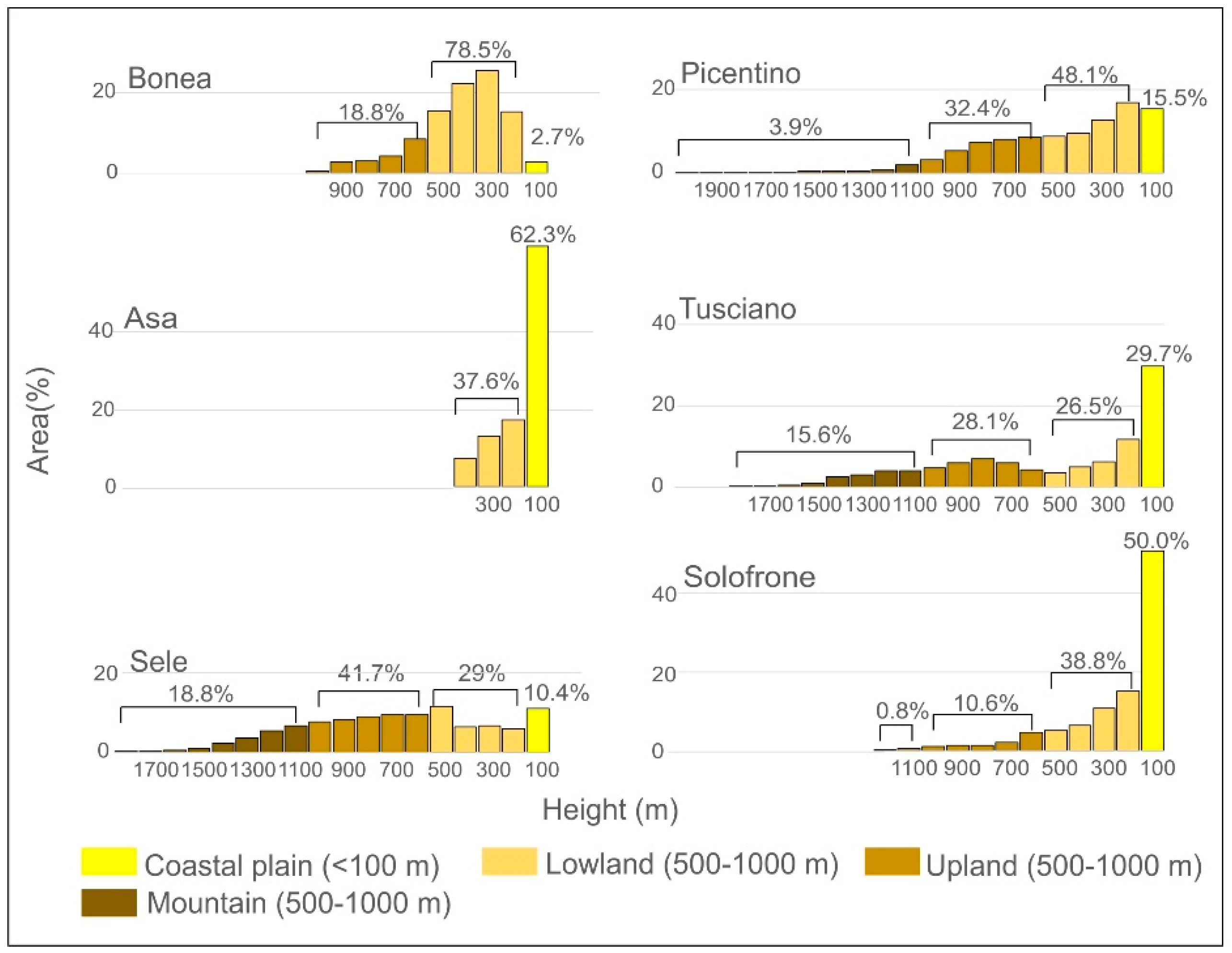
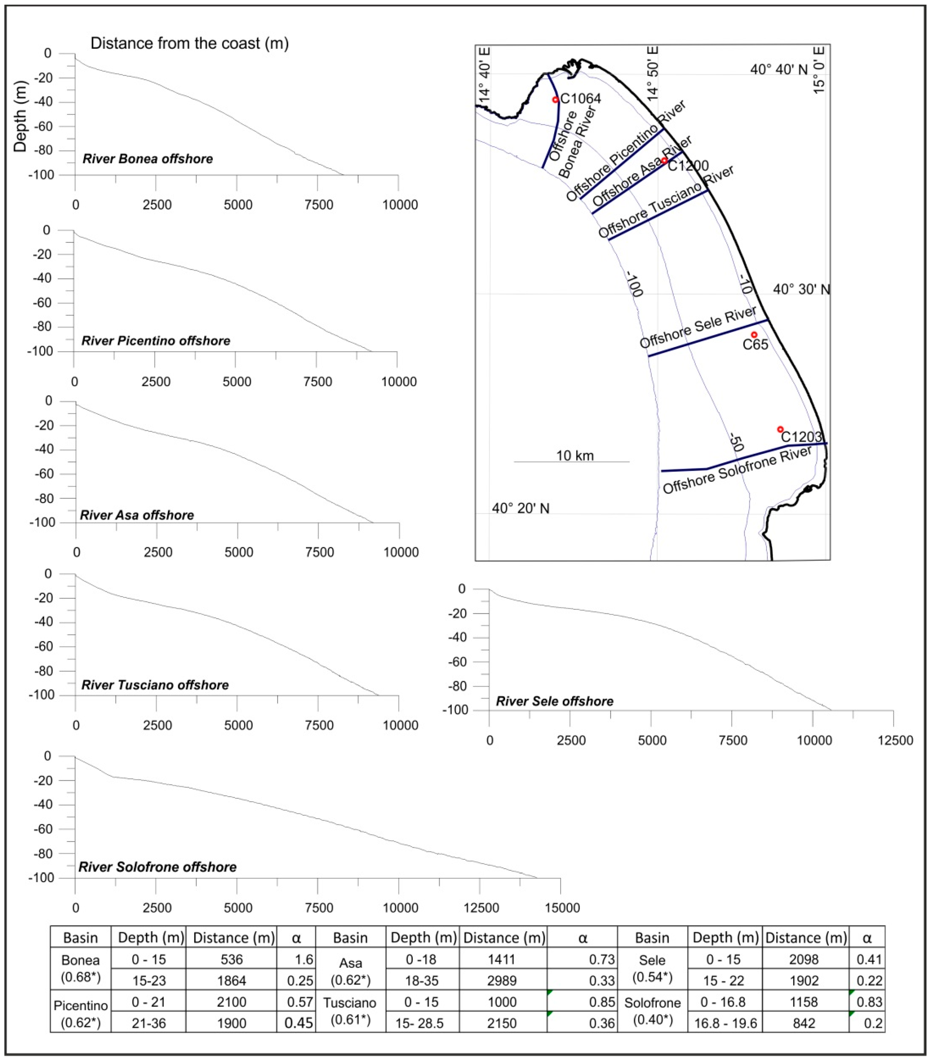
3.1. Watershed Morphology

The hypsometric curve of a catchment represents the relative area below (or above) a given altitude [54] which describes the distributions of elevations in a watershed. The curve is created by plotting the proportion of total watershed height against the proportion of total watershed area and it can have three main shapes. A convex profile identifies young slightly eroded regions, a “S” shaped curve characterizes moderately eroded regions and a concave curve typifies highly eroded regions [54].

The hypsometric curves for the SGCs were outlined in three main steps. The single hydrographic watershed was extracted from the Digital Elevation Model (DEM) of Campania Region with a resolution of 20 m per side (Figure 1), which is considered detailed for this type of analysis [55].

The area of each watershed (A) was reclassified into elevation classes of 100 m ($\mathrm{a}$) and for each one the elevation (h) was calculated as the mean value of the values identifying the single elevation classes. The parameter “a”, “h” and H, the maximum elevation of the basin, were used to calculate the rates ($\mathrm{x};\mathrm{y}$) illustrated in (1) and to draw the hypsometric curve:

$$x=\frac{a}{A}; y=\frac{h}{H}$$

(1)

Moreover, according to [56,57,58], to quantify the changes in the morphology of the drainage areas with similar hypsometric integral values, two dimensionless parameters were used, i.e., hypsometric skew and hypsometric kurtosis, derived from the distribution function of the hypsometric curve. The hypsometric skew is a defined as:

$$HypSkew=\frac{{\mu }_3}{{\sigma }^3},$$

(2)

where ${\mu }_3$ is the third moment calculated according to [56] and $\sigma$ is the square root of the variance. This parameter represents the amount of headward erosion in the upper reach of a watershed.

The hypsometric kurtosis is a defined as:

$$HypKurotsis=\frac{{\mu }_4}{{\sigma }^4},$$

(3)

${\mu }_4$ is the fourth moment calculated according to [56]. This parameter points out the erosion on both upper and lower reaches of a watershed.

The moments and the coefficient of skew and kurtosis were also defined for the density function of the hypsometric curve; the density skew denotes the slope change while the density kurtosis depicts mid- watershed slope.

We also calculated the Melton ratio (R) to comprehend if our watersheds were prone to flooding, debris flows or debris floods [24]:

$$R=\frac{H}{\surd A},$$

(4)

where H is the difference between maximum and minimum elevations in the watershed and A is the catchment area.

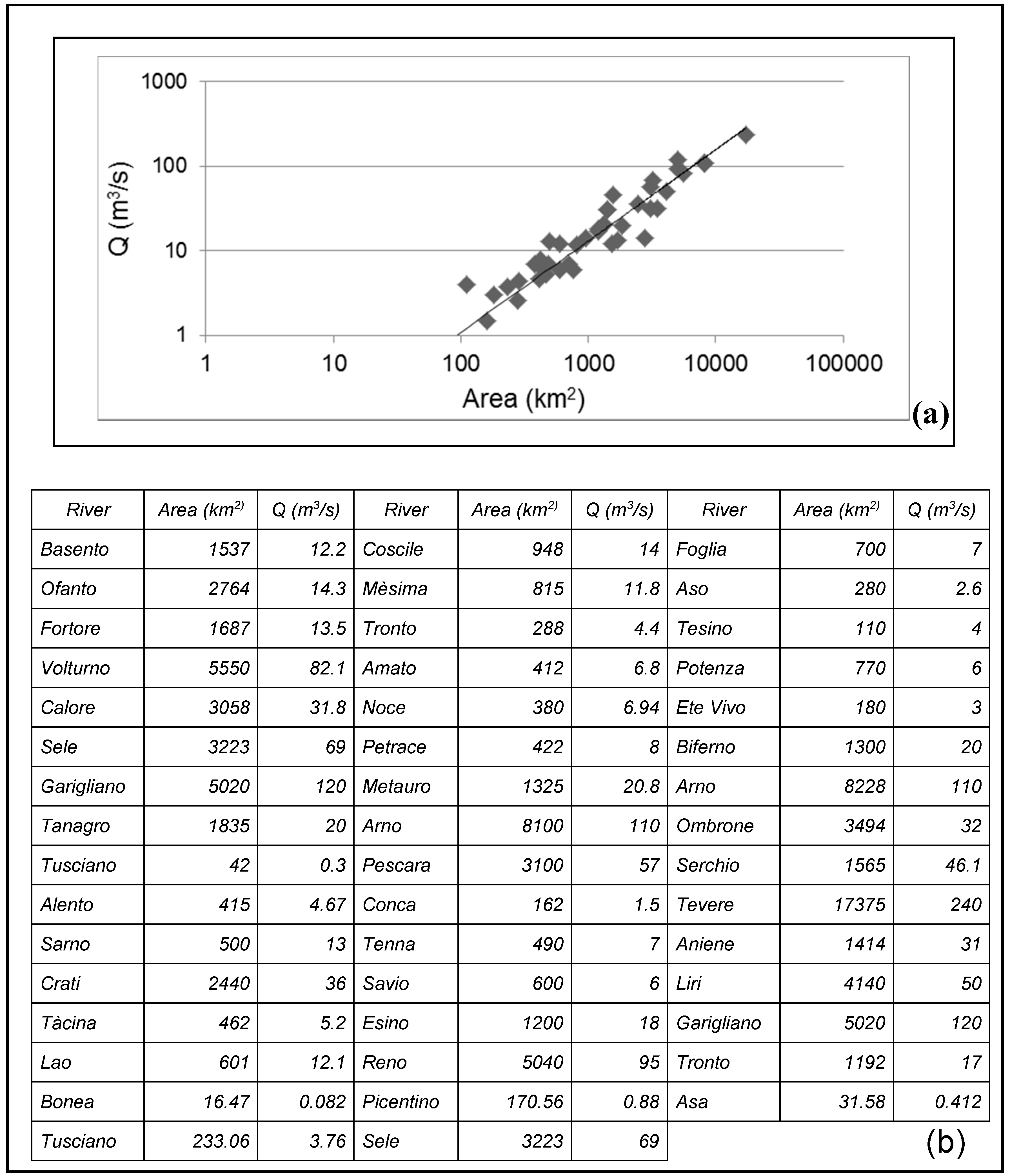
3.2. Rivers Discharge and Sediment Load

A river can produce HFs if the suspended sediment concentration (Cs_av, kg/m³) overcomes the critical sediment concentration (Cc, kg/m³), according to Mulder and Syvitski [18].

This assumption presumes prior conditions, i.e., that the sediment mass moved by rivers is entirely suspended at the river mouth and that the bedload transport is generally <10% of the total sediment transported by river at the mouth [18]. For the study area, as part of a temperate zone (Lat. 30°–50°), a Cc value of 42.74 kg/m³ [23] was adopted.

In the present work, the tendency of the SGCs river to produce HFs as a result of exceptional meteoric events, was analyzed. To achieve this goal, we used the nomogram published by [18], which requires as input data the values 1/Cs_av and Q_flood/Q_av, where Cs_av is the average suspended concentration (kg m⁻³), Q_flood is the maximum flood discharge (m³/s) and Q_av is the average river discharge (m³/s). These values were therefore calculated and reported in

Table 1. Data characterizing the rivers of the study area: (i) average suspended sediment load (Q_Sav), (ii) average discharge (Q_av), (iii) maximum flood discharge (Q_flood), (iiii) average suspended sediment concentration (C_Sav).

River Watersheds	Qsav (kg/s)	Qav (m3/s)	Qflood (m3/s)	Csav (kg/m3)
Bonea	8.32	0.08	12.49	101.44
Picentino	3.76	0.88	88.61	4.27
Asa	1.69	0.41	21.55	4.11
Tusciano	28.13	3.76	115.12	7.48
Sele	12.94	69.00	1086.06	0.19
Solofrone	1.03	1.30	59.48	0.79

.

The Cs_av parameter was calculated as the ratio between $Q{s}_{av}$ (average suspended sediment - kg/s) and Q_av.

The average suspended sediment was calculated by using empirical relation inferred from the analysis of world rivers database, published by Milliman and Syvitski [23] and modified by Mulder and Syvitski [18]:

$$Q{s}_{av}=c\times A^d,$$

(5)

where A is the catchment area (km²) and $c,$ $d$ are the regression coefficients varying in consequence of watershed morphology. For the Tusciano and Sele rivers, the coefficient “c” is equal to 4.31 and “d” to 0.29. For Bonea and Picentino the coefficient “c “is equal to 0.68 and “d” equal to −0.34, while for Asa and Solofrone rivers “c” is equal to 0.22 and “d” equal to −0.41. These values typify the three watershed categories “other mountains”, “upland” and “lowland” over the seven identified by Mulder and Syvitski [18].

The average river discharge (Q_av) data for SGCs rivers were recovered from the Water Management Plan of Southern Apennines Hydrographic District (2015–2021) [59]. Only for the Solofrone River it was calculated according to the experimental relation proposed by Syvitski and Milliman [60], which relates river discharge to catchment area, here modified considering the rivers of Southern Italy (Figure 3a,b), as follows:

$$Q=0.0125 A^{1.0182},$$

(6)

where A is the catchment area in km².

The maximum flood discharge ($Q_{flood}$), is strictly related to the watershed area (A), as highlighted by the following empirical relation:

$$Q_{flood}=a\times A^b,$$

(7)

where A is the watershed area in km² while a = 1.1922 and b = 0.8384 are two coefficients calibrated for the rivers of Campania region [61].

3.3. Marine Sediment Analysis

Offshore, the grain size analysis of 22 seabed samples (21 grabs and one box-core) and of four marine sediment cores (C1064, C1200, C65, C1203) were considered for the present study (Figure 1). The grabs and box core samples were taken between −14 and −100 m depth for geological mapping purposes in 2003 [35,62] while the cores C1064, C1200, C1203 were retrieved in 2002 between 1 and 3 km off the coastline at the river mouth of the main rivers and at water depth ranging between −22 to −29 m [21,63]. The core C65 was retrieved at lower depth (−14 m), off the Sele River mouth in 2000 [51]. Also, 31 grain size analysis were carried out on cores C1064, C1200 and C1203 sub-samples at least every 10 cm down-core, at the ISMAR CNR sedimentological Laboratory in Naples, to integrate those already available from references [51], reaching a total of 106 analyses. Sieve sifting separated the grain fractions of >4000 > 2000> 1000 > 500 > 250 > 125 > 90 > 63 > 30 µm. The residual water after sieving, containing the <30 µm fraction (fine silt and clay), was dried and weighed.

Grain size classes were grouped in >63 µm (sand) and ≤ 63 µm (mud) and the ratio between the percentage of sandy (S) and muddy (M) fractions at the sea bed were plotted versus the sampling depth, to assess the present-day relation at the seabed (hereafter, S/M_Depth). We assumed that this relation has been valid over the very recent past and thus it was used to calculate the expected S/M values every 10 cm down-core (S/M_Paleodepth). These values plus the SE characterizing the S/M_Depth relation, were compared to the S/M measured from the grain size analysis (S/M_Grainsize), performed every 10 cm, to evidence the anomalous event beds (S/M_Grainsize > S/M_Paleodepth + 2SE), down-cores. The analysis encompassed to the most the last 2 kyrs, according to the chronostratigraphic and chronologic age datings provided in Budillon et al. [51,63].

4. Results

The relation between the morphology of hydrographic watershed s and the occurrence of sandy-rich event beds as outliers with respect to the “normal” sedimentation, defined by the experimental low S/M_Depth into the shallow marine sediment record of the Salerno Gulf, is here discussed.

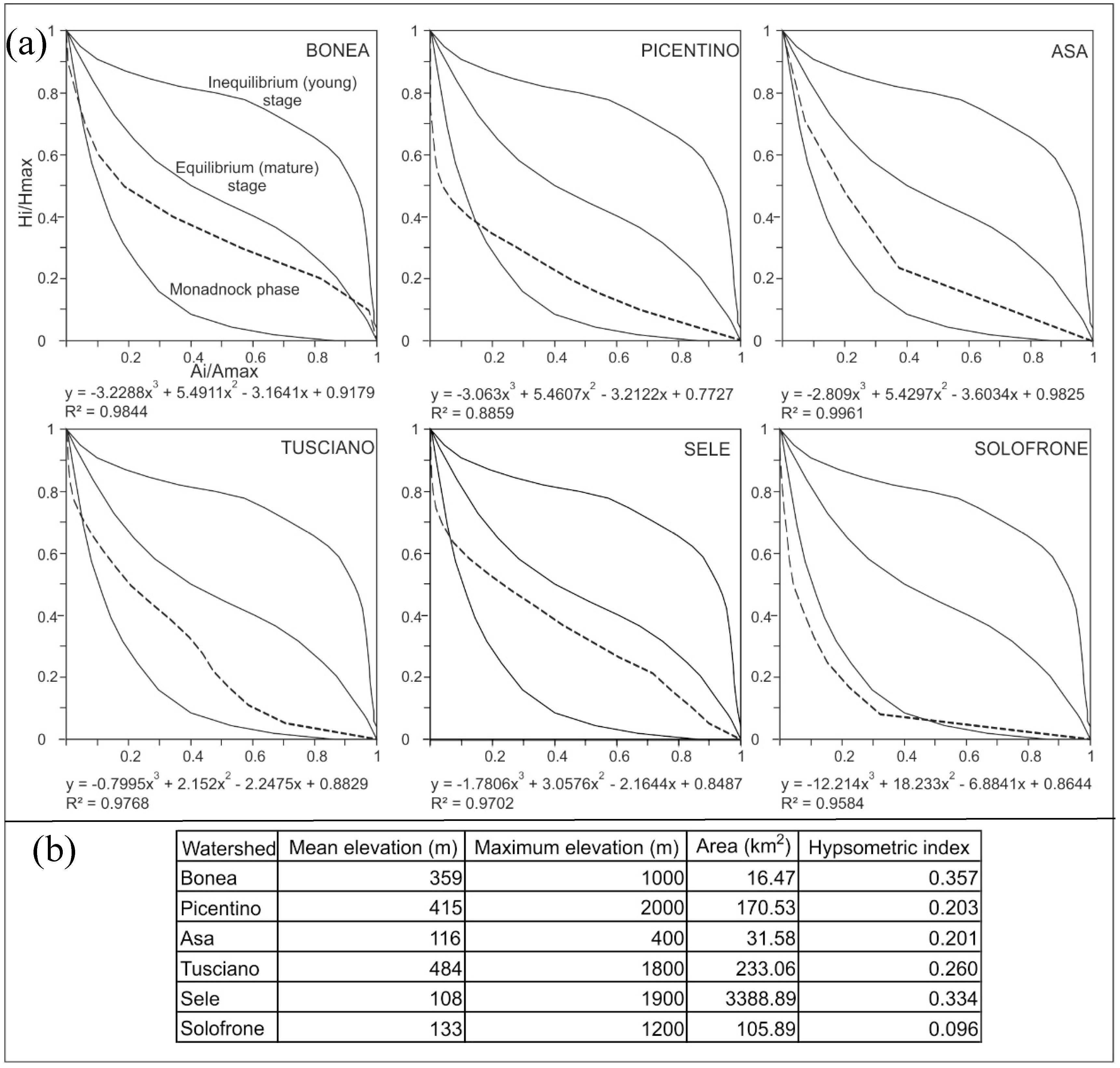
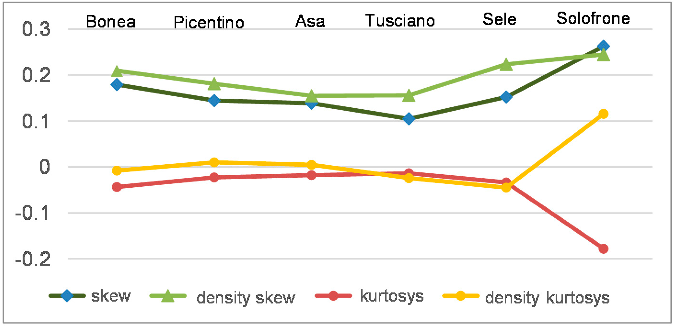
4.1. Hypsometric Analysis

The SGCs have an integral value ranging from 0.09 to 0.36 which indicates a mature stage. Nevertheless, a comparison of the single hypsometric curves with the three stages of geomorphic development of a watershed [64], revealed some differences (Figure 4).

The Bonea watershed has an elevation drop of 1000 m and an area of 16 km². About 78% of the watershed develops between 100–500 m a.s.l., 19% above 500 m and only 2.7% develops in the coastal area (Figure 5).

The hypsometric curve evidences a high gradient for hi/Hmax <= 0.7 and Ai/Amax <= 0.004, that slightly decreases from the latter point to the Ai/Amax = 0.2. After this point, the curve has a constant slope and appears close to the Equilibrium stage with Ai/Amax varying from 0.2 to 0.8 while it becomes convex for Ai/Amax varying from 0.8 to 1 (Figure 4).

The Picentino watershed has an elevation drop of 2000 m and an area of 170 km². About 40% of the watershed develops above 500 m a.s.l., of which 4% is higher than 1000 m; 48% of the watershed is between 500 and 100 m high and 15% is below the 100 m a.s.l. mark (Figure 5). The hypsometric curve shows a high gradient in its upper part from hi/Hmax <= 0.5 and Ai/Amax <= 0.1 (a restricted area) and becomes successively closer to the Monadnock phase with a concave shape that linearly decreases (Figure 4).

The Asa is a small watershed, with an elevation drop of 400 m and an area of 31 km². About 62% of watershed develops under 100 m in height (Figure 5). The hypsometric curve has a concave shape and presents a lower slope than the other watersheds for hi/Hmax <= 0.7 and Ai/Amax<= 0.2 but it is located above the Monadnock phase curve. A sector also characterized by high gradient follows (from Ai/Amax > 0.2 to Ai/Amax = 0.4) and decreases in the last part (Figure 4).

The Tusciano watershed has an elevation drop of 1800 m and an area of about 230 km². 44% of the watershed develops above 500 m a.s.l, of which 16% is higher than 1000 m a.s.l. and 30% is under 100 m in elevation (Figure 5). The hypsometric curve shows a high gradient in the upper zone (hi/Hmax <= 0.8 and Ai/Amax <= 0.1) a slope change in the middle sector (from Ai/Amax = 0.4 to 0.6) and ends with a concave shape (Figure 4).

The Sele watershed has an elevation drop of 1900 m and an area of about 3380 km². It is the biggest watershed of the study area with about 60% of the watershed developing above 500 m in height and 18% of that portion is higher than 1000 m. The catchment area also has about 29% of the territory developing in a low land zone, while 10% develops along the coastal area (Figure 5). The hypsometric curve has a high gradient for hi/Hmax <= 0.8 and Ai/Amax <= 0.02; it maintains a constant trend for Ai/Amax varying between = 0.2 and 0.7 and only subsequently shows a breaking slope (Figure 4).

The Solofrone watershed has an elevation drop of 1200 m and an area of about 105 km². 50% of the territory has an elevation that is less than 100 m, about 38% develops in a low land area and 11% at elevations higher than 100 m of which only 0.8% show elevations higher than 1000 m (Figure 5). The hypsometric curve shows high values with hi/Hmax <= 0.5. The Ai/Amax ranges between 0 and 0.1 but slightly decreases until Ai/Amax = 0.3 and successively keeps a constant low slope (Figure 4). The high gradient in the upper part of the hypsometric curves indicates that the amount of material left after erosion is smaller [54,56,57]; in other words the linear erosion and the slope erosion are balanced [65]. This status can be considered a sign of maturity for the watershed. Indeed, the lateral erosion was intensive in the river head [64,66].

The main statistical moments of the hypsometric curves served as tools to recognize differences among the SGCs with both a similar shape and integral values. The hypsometric skewness can be interpreted as the amount of headward erosion in the upper zone of watershed. Skewness equal to zero indicates that there are no masses undergoing erosional processes. The curve will become more and more positively skewed with headward development of the main stream and of its tributaries as these streams encroach on flat-upland parcels in the upper reaches of the watershed [56]. It was observed that when the integral decreases, the skewness value becomes larger. A value lower than 0.3 confirms a mature phase for all the investigated watersheds, however the skewness decreases moving from Solofrone to Bonea, Sele, Picentino, Asa and Tusciano watersheds.

The hypsometric kurtosis can be used to deduce if the erosion occurs in both the upper and lower reaches of a watershed. In this case the value of kurtosis is relatively high [56]. In SGCs this value is negative and close to 0; nevertheless, the Tusciano, Sele and Asa have higher values than Picentino, Bonea and Solofrone watersheds (Figure 6).

The density skew reveals the rate of change along the hypsometric function. The more rapid is the change, the higher the density. A density skewness equal to 0 indicates an equal amount of change characterizing the upper and lower reaches. This value is close to 0 for all SGCs. Rapid change from mountain to upland area typify the Solofrone followed by Sele and Bonea watersheds (Figure 6).

The density kurtosis delineates mid-watershed slope. All watersheds have values close to 0 however, for the Sele Tusciano and Bonea it is slightly lower than 0, indicating that slope change characterizes the upper and lower reaches of watersheds (Figure 6). In particular, a slope change characterizes: a) the Sele watershed between 1876 and 1400 m a.s.l. and from 400 to 100 m a.s.l.; b) the Tusciano watershed in the upper and middle parts of watershed; c) the Bonea watershed in the upper and lower part (between 300 m a.s.l. and the mouth) (Figure 4).

The Picentino and the Asa catchment areas show slope change only in the upper part of the watersheds and a constant gradient trend of hypsometric curves after 1000 m a.s.l. for the first and 100 m a.s.l. for the second, respectively (Figure 4). The Solofrone watershed shows one slope change at about 100 m a.s.l. where it becomes flatter (Figure 4).

Moreover, we defined the Melton Ratio to rapidly identify the dominant sediment-transport processes (e.g., debris-flow, debris-flood, and flood) in our watersheds. This rate, with a value of <0.30, indicates that conventional fluvial processes are generally the dominant fan-forming processes [24].

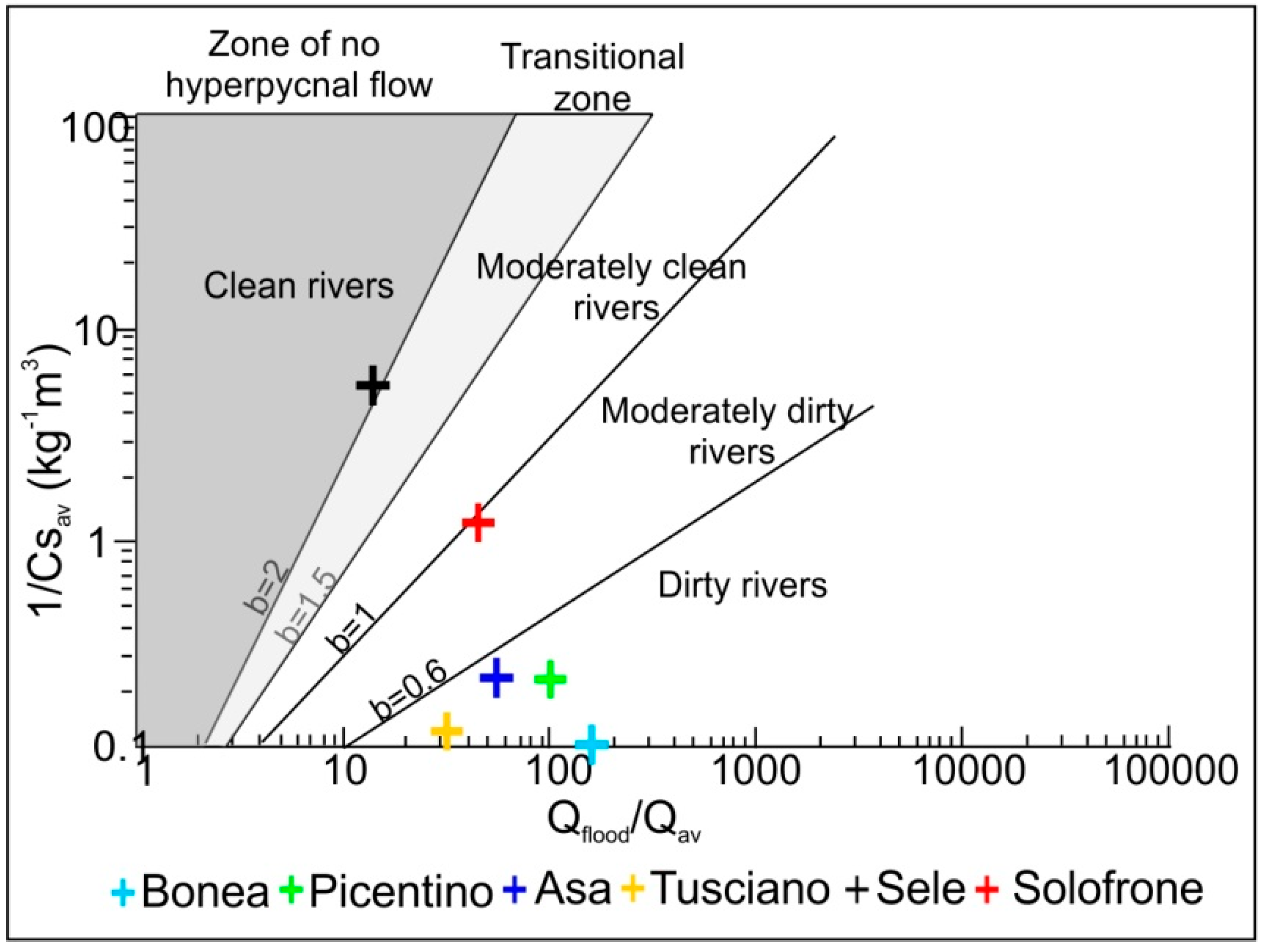
4.2. Hyperpycnal Flows

To evaluate the tendency of SGBs to produce HFs during the intense rainfall, the values 1/Cs_av and Q_flood/Q_av, calculated for each examined river (Table 1), in the nomogram proposed by [23] were plotted (Figure 7).

The diagram shows a tendency of the Bonea, Picentino, Tusciano and Asa rivers (all of which fall into the “dirty river zone” markedly below the “b” value equal to 0.6) to produce hyperpycnal plumes. The Solofrone River, falling in the zone of “moderately dirty river” is also prone to producing HFs, but possibly with longer recurrence times [18]. The Sele River—falling into the zone of “no hyperpycnal flow”—should not generate HFs at all (Figure 7).

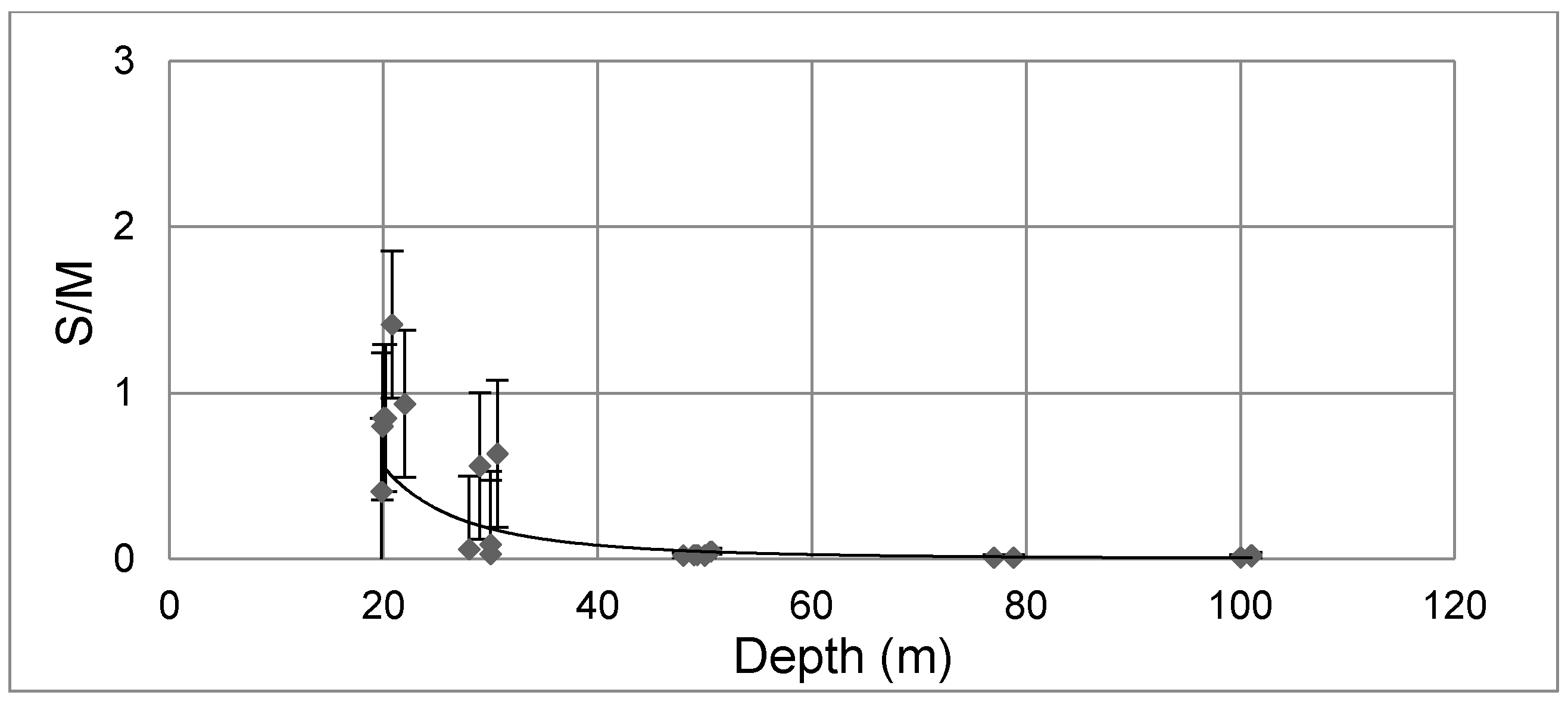
4.3. Grain Size of Marine Sediment and Depth Correlation

The experimental relation S/M_Depth was defined on the base of the grain size analysis of the seabed samples retrieved between −14 m and −100 m in the continental shelf of the Salerno Gulf. It has the form of $y=2109x^{-2.751}$ and has a regression coefficient (R) of 0.76 and a standard error (SE) of 0.376 that slightly increases to 0.44 in the first 30 m depth and decreases to 0.03, from 30 to 60 m, and to 0.006 at higher depth (Figure 8).

We limited the analysis to the −14 m/−100 m depth range for three main reasons: (i) at shallower depth the lateral variability of sediment grain size is modulated by submerged beach processes, alongshore currents and delta front deposition; (ii) at depth greater than −100 m, patches of relict sand may outcrop at the seabed, thus biasing the validity of the relation; (iii) the stratigraphic record examined in this study through the analysis of the cores is relative to a continental shelf environment, thus it has to be compared to a current analogous counterpart.

It was also assumed that, for each examined down-core layer, the relation between S/M and its paleo-depth (i.e., the present-day core depth below sea level + the layer depth below sea floor), had been regulated by the S/M_Depth relation observed currently at the seabed (Figure 8). This assumption is grounded on the consideration that the examined cores encompass no more than the last 2 kyr, according to the datings proposed in [21,51,63], a time span in which the environmental conditions have not changed significantly. The S/M_Grainsize, measured down-core and plotted against the paleo-depth, showed the variability of the sediment texture over the last two millennia in the Salerno Gulf (Figure 9). The outliers, i.e., those samples with S/M_Grainsize overcoming the threshold value (S/M_Depth + 2SE), mark the occurrence of event beds whose deposition can be accounted by HF processes at the river mouths (see discussion). The threshold value (green line in Figure 9) changes with paleodepth as it is a function of depth.

Samples from core C1064 (collected 2.84 km off the coast of the Bonea watershed), from core C1200 (collected from the front of Picentino-Asa-Tusciano watersheds 2.0 km off the coast) and from core C1203 (collected from the front of the Solofrone watershed, 3.55 km off the coast) (Figure 9), were examined. The samples of core C65 off the Sele River mouth were not considered for three main reasons: (i) the morphological analysis of the watershed and the position in the nomogram of Figure 7 evidenced that the Sele River is not prone to producing HF; (ii) core C65 was retrieved at −14 m, i.e., in a setting too close to the river mouth sand bar and thus influenced by the riverine bedload processes; (iii) the SE value at −14 m depth is as high as 1.4, and possible depositional anomalies would be blurred by the natural grain size variability at that depth.

The S/M_Grainsize plotted in the bar diagrams of Figure 9 evidence several down-core anomalies, i.e., values overcoming the threshold value (green line) relative to the depth of the considered subsample (paleodepth in m b.s.l.). A cluster of anomalies is grouped in the uppermost part of the cores (C1, C4, C6, in core C1064, C2 in C1200 core, D4 in C1203 core), whereas a substantially flat trend is registered in the middle part of each core. Toward the base of the cores, C1064 shows the A4, A8 and A11 anomalies, while C1200 shows the A22, A25, A28, A31, A37 and A40 anomalies and C1203 core shows the C19, C21, B23, B25, B31, A36, A40 anomalies. This concentration of events at the base of the cores is not accidental, and is due to the coarse grained content of these horizons which have limited the penetration of the core barrels further in depth.

The anomaly A40 in C1203 registers the fall-out event of the Mt Somma-Vesuvius Plinian eruption in 79 AD and A22 in core C1200 indicates the eruption from the same vent in 620 AD [51]. The anomalies A37, A31, A28 and A25, below the 640 AD tefra layer in C1200, mark very coarse-grained and poorly sorted deposits made of heterogenic gravel with outsized clasts within an oxidized sandy matrix, virtually incompatible with HF processes s.s..

It was observed that the anomalous S/M_Grainsize layers in cores C1200 and C1203 are comparable in thickness, each almost exceeding 20 cm. In C1064 with the exception of the C6 event, the remaining detected events are all under 10 cm in thickness.

The largest event beds show a clear coarsening upward and a fining upward texture and in some places, symmetrical shapes and gradual transitions (C2, A25, A36). In other sections the event beds have an asymmetrical shape with a steep base and a less steep fining upward trend.

The C4–C6 anomaly in C1064 exhibits a double peak feature that may suggest a complex depositional signature, including double stacked normally graded units above an inverse graded unit based by a gradual transition [69]. The thinnest events (C1, A4, A8, A11 in C1064; A40 in C1200; C19 in C1203) are often represented by a single or double peak over the threshold and do not allow for effective observations.

The 2–4 m deep interval in C1203 registers a set of different events overlaying one another and no fine-grained intervals have been preserved. Given the down-core sub-sampling rate (each 10 cm, excluding the lower part of C1200 which was sampled each 5 cm), it is possible that the minor event beds have not been detected by the analysis.

5. Discussion

5.1. Analysis of SGCs Morphology and Its Role in Promoting HF Events

The role played by the morphology of SGCs in promoting the HF events is here discussed.

The Sele River watershed, the largest in the study area, has a wide coastal plain (about 10%) continuing inland with a lowland area representing about 30% of its extension (Figure 5). These two zones contribute to a reduction of relief energy and promote the deposition of material eroded from the headwater as pointed out by the hypsometric skew. The density skew indicates a rapid elevation change from mountain to upland zone (Figure 6), where the energy of the river catchment is reduced as testified by the density kurtosis (Figure 6).

The shape of the Asa river catchment and relative indexes reinforce the concept that it is part of the moderately clean river. It has an elevation drop of only 400 m and the greatest part (about 62%) of watershed develops in coastal plain (Figure 5). The density kurtosis points out a slope change only in the upper part of the watershed (Figure 6). Indeed, the shape of the hypsometric curve is constant from the 100 m elevation to the outlet (Figure 4).

The Solofrone river catchment is characterized by similar features but it has more relief energy (elevation drop of 1200 m) and a high gradient for mountain and upland zones (see hypsometric curve, Figure 4) where the erosion is active (hypsometric skew, Figure 6).

The Picentino river catchment, has an elevation drop of 2000 m and about 40% of the watershed develops above 500 m (Figure 5); the hypsometric curve shows a high gradient only in its upper part (Figure 4) where erosion is active (hypsometric skew, Figure 6). Similar features characterize the Tusciano river catchment which unlike the Picentino river catchment, presents a slope change in the middle part that feeds new energy to the system as testified by the density kurtosis (Figure 6). Moreover, this watershed shows the lowest head erosion rate (hypsometric skew, Figure 6).

5.2. Age Constraint of the Event Beds.

Alas, no age model of cores is available up to date. However, according to recent studies based on integrated stratigraphy (geochronology, tephrostratigraphy and physical properties correlations) on the same cores [21,51,63], it has been possible to constrain some of the event beds to specific time intervals.

In particular, the deposits corresponding to peaks C6 in core C1064 (Figure 9) are the HFD relative to the 1954 flood of the Bonea River that hit Vietri sul Mare village off the city of Salerno [21,68,70]. Furthermore, the lower part of core C1064 is related to the 15th century, while the layer at −100 cm b.s.f. is related to the 18th century (Figure 9) [21]. In C1200 the lowermost 50 cm settled before 620 AD, as testified by the occurrence of a fall-out tephra from Mt. Vesuvius [51]. In C1203 the lowermost 2 m of sediment were deposited between the 1st century and the 17th century, whereas the uppermost 2 m were deposited in the last four centuries [51].

Consequently, the lower cluster of anomalies (A4, A8, A11) in C1064 span within the 15th–8th century time frame, and the lower cluster of anomalies (B23, B25, B31, A36) in C1203 span within the 79 AD–17th century time frame. The anomalies in C1200 core (A25, A28, A31, A37, A40), predating 620 AD, record a dramatic lithologic transition. According to the sequence stratigraphic analysis in Budillon et al. [51], based on very high resolution seismic interpretations, they are relative to a previous systems tract lying below the subaerial unconformity of the Upper Pleistocene. Thus the lithologic transition at about −2.30 m bsf includes a large stratigraphic hiatus. Therefore, as these deposits are not representative of present-day/recent environmental conditions, they were not further investigated in our analysis. The observations point to a clear mismatch of the occurrence of anomalous events among cores, with the exception of those for modern time.

5.3. The Anomalous S/M Layers Occurrence in the Marine Sink

The occurrence of unusual coarse-grained beds (hyperpycnites, tempestites, tsunamites, deposits from submarine delta front failure) in the shallow marine sediment record below the closure depth, has been long discussed [71,72] in the last decades and it is nowadays a main issue, since it relates to coastal hazard management.

We did not consider the tsunami waves as a potential mechanism generating the analyzed deposits in the last 2 kyr because, according to Alberico et al. [73], the studied area resulted as being almost completely sheltered or too distant with respect to the great number of possible tsunami-source areas identified in the Western Mediterranean Sea thus far.

Sand-rich layers interbedded with mud in the continental shelf stratigraphic record are normally regarded as a proxy for past storms. In fact, the intense cyclonic circulation at middle latitudes may trigger the deposition of down-welling currents originated by sea-storms [74], HFs at the mouth of flood-prone rivers [18] and may also induce instability along the high gradient delta fronts, if overcharged by a sudden sediment load (not discussed in this study). The first two processes are particularly effective in delivering huge amounts of sand to the neritic environment, with possibly very similar lithologic features [63].

Most of the diagnostic elements for recognizing hyperpycnal flow deposits (HFD) are provided by inland observations at the field scale and refer to sustained hyperpycnal flows [75,76,77]. Thus, there is a practical difficulty in distinguishing hyperpycnal flows from tempestite deposits on modern shelves by standard marine investigations (cores analysis and seismic surveying), possibly because the interpretation is biased by the resolution of the seismic investigations and because of the limited extension of the lithofacies observations. Furthermore, in the Mediterranean region major sea-storms, related to cyclonic circulation, are often accompanied by cold fronts inducing heavy rainfall and cloudburst [17,78,79,80]. This last point is of main relevance, because in relatively-small catchments (<10³ km²) floods are normally short-lived (from few hours to max. 2–3 days) and the sediments transported from the source areas downstream, during the flood conditions, are delivered into the marine sink in a short time, when rough sea conditions are very likely still active [81,82,83]. In these cases, both processes may couple in delivering and reworking sand beyond the littoral strip [84]. Thus, flood sediments are widely dispersed and resultant beds are likely to be relatively thin compared to the involved material at the fluvial outlet, and the settled deposits could be almost completely homogenized [85,86], at least in the range depth where storm conditions are still impactful. A numerical modelling of the coastal circulation and sediment transport under sea-storm conditions in the Salerno Gulf has shown that the magnitude of the combined wave-current shear velocity might set in motion the fine sands down to about 37 m of depth [87]. We believe that these conditions (hyperpycnal flow and sea storminess) are the environmental forcing factors that have driven the settlement of sand-rich layers in the Salerno Gulf at depth.

The application of the experimental power relation S/M_Depth to the paleodepth allows to identify the depositional anomalies in the sediment record and can provide an objective evaluation of the variances to the fair weather deposition occurring in the shallow water sinks. The S/M_Grainsize anomalies identified in the investigated cores of the Salerno Gulf vary between 1 and 7: (i) in the Bonea offshore, 5 events over 5 centuries have been detected; (ii) in the Asa - offshore 1 event over about 14 centuries has been detected and (iii) in the Solofrone offshore at least 7 events in the last 19 centuries have been recorded. Thus a recurrence time of about 0.1 kyr can be inferred for the catchments of the Bonea river which has been classified as a “dirty river”; a recurrence time of about 0,3 ky can be estimated for the Solofrone river catchment, which results as being a “moderately clean river” (Figure 7). No direct corroboration can be assumed for the Tusciano and Picentino river catchments, since the C1200 core is directly facing the Asa river mouth and possibly it would not register HFs generated by laterally displaced river mouths. However, based on the nomogram of Figure 7 and considering the morphometric analysis of the watersheds it is reasonable to infer a return period of major HF events as short as that of the Bonea River.

The Asa River shows a trick recurrence time of about 1 kyr even if its falls in the field of “dirty rivers”. This anomaly can be accounted for by the wider extension of the coastal plain (topographic height ≤ 100 m a.s.l.) which exceeds 50 % of its territory (Figure 5). Moreover, off the Asa River mouth the seabed slopes by an angle of 0.33, steeper than the other sectors in the same depth range (Figure 10). These peculiar features may affect the run-out of any HF favouring the dispersal of riverine sediments at higher depths.

Certainly, many accidents could affect the preservation of the HFD after their deposition, as for instance the occurrence of a major HF event shortly afterwards, may overprint the previous one. On the other hand, when floods occur episodically, with long periods between consecutive flood events, their deposits may be extensively reworked before burial below the mixing layer [28] and therefore their fingerprint in the stratigraphic record could be eased. In fact, according to Wheatcroft and Drake [88] and Kniskern et al. [28] the preservation of the flood signal may be theoretically possible over the shelf depocentres where the flood layers exceeded 4.5 cm and accumulation rates exceeded 1 cmyr⁻¹, assuming a mixing layer thickness of 10 cm due to bioturbation [89]. In this regard, the Bonea offshore would offer the better conditions to preserve event beds, since an average accumulation rate of 2 cmyr⁻¹ can be evaluated over the last 5 kyr at −25 m of depth, whereas the Solofrone offshore should provide the worst conditions as it experienced a depositional rate of less than 0.6 cmyrs^-1 over the last 5 kyr.

The other factor that might affect the deposition of high S/M layers in this area is the high gradient of the continental shelf (Figure 9) that enables long runout and favors a reduced mass deposition in the transient sink [90]. The most significant effects might have impacted more the continental shelf facing the Asa River which has a slope gradient (value = 0.33) twice as much as the others in the first 500 m from the outlet and in the water depth 0–15 m.

The C1203 core registers a greater number of anomalous S/M_Grainsize layers especially in the lower section, despite the longer recurrence times of possible floods events (three times longer than that at the Bonea catchment). The anomalous S/M_Grainsize layers are overlay one another and no muddy interval is interbedded between them. In the Solofrone offshore a much reduced gradient of the seabed and a greater distance of the shelf break (>35 km) than that off the Bonea, Asa, Tusciano and Picentino rivers (about 10 km) can be observed. The peculiar topography of the seabed favors the settlement in shallow waters of S/M_Grainsize anomalies by lowering the speed of the fluxes due to frictional forces [25]. In addition, sandy deposits might aggrade at the seabed with higher thickness, provided that sufficient accommodation space is available [90]. The lack of fine grained deposits and the amalgamation of the sandy S/M_Depth layers in the southern sector of the gulf is not easily explainable. In fair-weather conditions the main circulation pattern of the alongshore currents follow an anticlockwise direction [91]. This condition may induce a drift of the estuarine plumes towards the north and therefore a negative balance of the fine grained sediment deposition with a consequent relative prevalence of sand in the coastal system in the southern sector of the gulf.

It is worth noting that the numerical method here developed to identify the anomalous S/M_Grainsize layers is affected by a variable accuracy in function of the depth. The accuracy in fact improves when it is applied to cores retrieved in deeper waters (30–70 m of depth), for which a SE error of the S/M_Depth experimental relation ranges between 0.03 and 0.006 (green line narrowing with depth—Figure 9). Moreover, in this depth range, the shelf profile often provides a natural morphological bowl to accommodate sediments, preventing post-depositional erosional processes [92,93].

6. Conclusions

A comprehensive knowledge of the land-to-sea processes is crucial in order to assess a proper management and to improve the resilience of coastal areas.

In the present work we evaluated the tendency of three categories of Southern Apennines watersheds—very small (Asa e Bonea), small (Tusciano, Solofrone and Picentino) and medium (Sele) —to trigger HF events, by integrating the morphometric analysis of river catchments with the quantitative analysis of marine cores in the shallow water environment, in line with the source to sink paradigm.

The morphometric indexes point out the mature stage and the dominance of the fan-forming processes driven by flooding events (Melton ratio ≤ 0.3) of all the examined watersheds. Four of the six examined rivers however resulted as being dirty rivers, one “moderately dirty” and only one fell into the “no HF” category, according to the Mulder and Syvitski nomogram, regardless of the dimension of the catchment itself.

The S/M_Depth experimental relation applied to the marine cores led to infer a HF event recurrence time of about 0.1 kyr for the category “dirty rivers” (Bonea, Picentino and Tusciano river catchments) and of about 0.3 kyr for the category “moderately dirty rivers” (Solofrone river catchment). The first group shows a hypsometric index ranging between 0.2 and 0.3, a low gradient coastal plain not exceeding 30% and a maximum topographic height ≥ 1000 m. The Solofrone river catchment has a hypsometric index ranging between 0.09 and 0.2. and about 50% of it develops in a low gradient coastal plain. The Asa watershed, despite being classified as a “dirty river”, shows a much lower recurrence time (>1 kyr); this occurrence can be accounted for by the great extension of the coastal plain (>63% of the total area) and by the reduced maximum elevation (≤400 m).

In the marine environment it has also been observed that continental shelves with high slopes favour the deposition of thin HFDs in marine sinks, whereas gentle sloping continental shelves seem to favour thicker (>20 cm) HFDs.

The method here proposed corroborates the effectiveness of the source to sink approach in which the observations made on land and offshore have been complemented to reach a more comprehensive vision of coastal area evolution. The quantitative analysis performed on marine cores is applicable to analogous sediment records in temperate continental shelves which encompass the last 3 kyr, a time interval in which the oscillations of relative sea level can be overlooked.

References

1. Guzzetti, F.; Reichenbach, P.; Cardinali, M.; Galli, M.; Ardizzone, F. Probabilistic landslide hazard assessment at the basin scale. Geomorphology 2005, 72, 272–299. [Google Scholar] [CrossRef]
2. Vennari, C.; Parise, M.; Santangelo, N.; Santo, A. A database on flash flood events in Campania, southern Italy, with an evaluation of their spatial and temporal distribution. Nat. Hazards Earth Syst. Sci. 2016, 16, 2485–2500. [Google Scholar] [CrossRef]
3. Doswell, C.A. Hydrology, floods and drought/ Flooding. In Encyclopedia of Atmospheric Sciences, 2nd ed.; Elsevier: Amsterdam, The Netherlands, 2015; pp. 201–208. ISBN 978-0-12-382225-3. [Google Scholar]
4. Borga, M.; Boscolo, P.; Zanon, F.; Sangati, M. Hydrometeorological analysis of the 29 August 2003 flash flood in the Eastern Italian Alps. J. Hydrometeorol. 2007, 8, 1049–1067. [Google Scholar] [CrossRef]
5. Merheb, M.; Moussa, R.; Abdallah, C.; Colin, F.; Perrin, C.; Baghdadi, N. Hydrological response characteristics of Mediterranean catchments at different time scales: A meta-analysis. Hydrol. Sci. J. 2016, 61, 2520–2539. [Google Scholar] [CrossRef]
6. Mulder, T.; Syvitski, J.P.M.; Migeon, S.; Faugeresa, J.C.; Savoyed, B. Marine hyperpycnal flows: Initiation, behavior and related deposits. A review. Mar. Pet. Geol. 2003, 20, 861–882. [Google Scholar] [CrossRef]
7. Katz, T.; Ginat, H.; Eyal, G.; Steiner, Z.; Braun, Y.; Shalev, S.; Goodman-Tchernov, B.N. Desert flash floods form hyperpycnal flows in the coral-rich Gulf of Aqaba, Red Sea. Earth Planet. Sci. Lett. 2015, 417, 87–98. [Google Scholar] [CrossRef]
8. Casalbore, D.; Chiocci, F.L.; Scarascia Mugnozza, G.; Tommasi, P.; Sposato, A. Flash-flood hyperpycnal flows generating shallow-water landslides at Fiumara mouths in Western Messina Strait (Italy). Mar. Geophys. Res. 2011, 32, 257–271. [Google Scholar] [CrossRef]
9. Pierdomenico, M.; Casalbore, D.; Chiocci, F.L. Massive benthic litter funnelled to deep sea by flash-flood generated hyperpycnal flows. Sci. Rep. 2019, 9, 5330. [Google Scholar] [CrossRef]
10. Esposito, E.; Porfido, S.; Violante, C.; Molisso, F.; Sacchi, M.; Santoro, G.; Spiga, E. Flood risk estimation through document sources analysis: The case of the Amalfi rocky coast. In Marine Research at CNR, Marine Geology; Brugnoli, E., Cavarretta, G., Mazzola, S., Trincardi, F., Ravaioli, M., Santoleri, R., Eds.; Marine Research at CNR: Rome, Italy, 2011; pp. 1–12. ISSN 2239-5172. [Google Scholar]
11. Santo, A.; Di Crescenzo, G.; Del Prete, S.; Di Iorio, L. The Ischia Island flash flood of November 2009 (Italy): Phenomenon analysis and flood hazard. Phys. Chem. Earth 2012, 49, 3–17. [Google Scholar] [CrossRef]
12. Alessio, G.; De Falco, M.; Di Crescenzo, G.; Nappi, R.; Santo, A. Flood hazard of the Somma-Vesuvius region based on historical (19–20th century) and geomorphological data. Ann. Geophys. 2013, 56, S0434. [Google Scholar] [CrossRef]
13. Chirico, G.B.; Di Crescenzo, G.; Santangelo, N.; Santo, A.; Scorpio, V. Alluvial fan flooding hazard: The study case of Teglia (San Gregorio Magno, Salerno). Rend. Online Soc. Geol. It. 2012, 2, 456–458. [Google Scholar]
14. Santo, A.; Santangelo, N.; Di Crescenzo, G.; Scorpio, V.; De Falco, M.; Chirico, G.B. Flash flood occurrence and magnitude assessment in an alluvial fan context: The October 2011 event in the Southern Apennines. Nat. Hazards 2015, 78, 417–442. [Google Scholar] [CrossRef]
15. Santangelo, N.; Santo, A.; Di Crescenzo, G.; Foscari, G.; Liuzza, V.; Sciarrotta, S.; Scorpio, V. Flood susceptibility assessment in a highly urbanized alluvial fan: The case study of Sala Consilina (southern Italy). Nat. Hazards Earth Syst. Sci. 2011, 11, 2765–2780. [Google Scholar] [CrossRef]
16. Santangelo, N.; Daunis-i-Estadella, J.; Di Crescenzo, G.; Di Donato, V.; Faillace, P.; Martin-Fernandez, J.A.; Romano, P.; Santo, A.; Scorpio, V. Topographic predictors of susceptibility to alluvial fan flooding, Southern Apennines. Earth Surf. Proc. Land. 2012, 37, 803–817. [Google Scholar] [CrossRef]
17. Violante, C.; Braca, G.; Esposito, E.; Tranfaglia, G. The 9 September 2010 torrential rain and flash flood in the Dragone catchment, Atrani, Amalfi Coast (southern Italy). Nat. Hazards Earth Syst. Sci. 2016, 16, 333–348. [Google Scholar] [CrossRef]
18. Mulder, T.; Syvitski, J.P.M. Turbidity currents generated at river mouths during exceptional discharges to the world oceans. J. Geol. 1995, 103, 285–299. [Google Scholar] [CrossRef]
19. Porfido, S.; Esposito, E.; Mazzola, S.; Violante, C.; Santoro, G.; Spiga, E. Frane ed alluvioni nel salernitano e a Cava de’ Tirreni 9-31. In Lo Alluvione, il Disastro del 1773 a Cava tra Memoria Storica e Rimozione; Foscari, G., Esposito, E., Mazzola, S., Porfido, S., Sciarotta, S., Santoro, G., Eds.; Edisud: Bari, Italy, 2013; pp. 9–31. ISBN 978-88-95154-87-9. [Google Scholar]
20. Porfido, S.; Esposito, E.; Molisso, F.; Sacchi, M.; Violante, C. Flood historical data for flood risk estimation in coastal areas, eastern Tyrrhenian Sea, Italy. Landslide Sci. Pract. Complex Environ. 2013, 5, 103–108. [Google Scholar]
21. Budillon, F.; Violante, C.; Conforti, A.; Esposito, E.; Insinga, D.; Iorio, M.; Porfido, S. Event beds in the recent prodelta stratigraphic record of the small flood-prone Bonea Stream (Amalfi Coast, Southern Italy). Mar. Geol. 2005, 222–223, 419–441. [Google Scholar] [CrossRef]
22. Porfido, S.; Esposito, E.; Alaia, F.; Molisso, F.; Sacchi, M. The Use of Documentary Sources for Reconstructing Flood Chronologies on the Amalfi Rocky Coast (Southern Italy). Geohazard in Rocky Coastal Areas; Special Publications; The Geological Society: London, UK, 2009; Volume 322, pp. 173–187. [Google Scholar] [CrossRef]
23. Milliman, J.D.; Syvitski, J.P.M. Geomorphic/tectonic control of sediment discharge to the ocean: The importance of small mountainous rivers. J. Geol. 1992, 100, 525–544. [Google Scholar] [CrossRef]
24. Wilford, D.J.; Sakals, M.E.; Innes, J.L.; Sidle, R.C.; Bergerud, W.A. Recognition of debris flow, debris flood and flood hazard through watershed morphometrics. Landslides 2004, 1, 61–66. [Google Scholar] [CrossRef]
25. Zavala, C.; Pan, S.X. Hyperpycnal flows and hyperpycnites; Origin and distinctive characteristics. Lithol. Reserv. 2018, 30, 1–27. [Google Scholar]
26. Warrick, J.A.; Barnard, P.L. The offshore export of sand during exceptional discharge from California rivers. Geology 2012, 40, 787–790. [Google Scholar] [CrossRef]
27. Mathalon, A.; Goodman-Tchernov, B.; Hill, P.; Kálmán, Á.; Katz, T. Factors influencing flashflood deposit preservation in shallow marine sediments of a hyperarid environment. Mar. Geol. 2019, 411, 22–35. [Google Scholar] [CrossRef]
28. Kniskern, T.A.; Mitra, S.; Orpin, A.R.; Harris, C.K. Characterization of a flood-associated depositon the Waipaoa River shelf using radioisotopes and terrigenous organic matter abundance and composition. Cont. Shelf Res. 2014, 86, 66–84. [Google Scholar] [CrossRef]
29. Shanmugham, G. The hyperpycnite problem. J. Palaeogeogr. 2018. [Google Scholar] [CrossRef]
30. Carter, L.; Milliman, J.D.; Talling, P.J.; Gavey, R.; Wynn, R.B. Near-synchronous and delayed initiation of long run-out submarine sediment flows from a record-breaking river flood, offshore Taiwan. Geophys. Res. Lett. 2012, 39, L12603. [Google Scholar] [CrossRef]
31. Warrick, J.A.; Simms, A.R.; Ritchie, A.; Steel, E.; Dartnell, P.; Conrad, J.E.; Finlayson, D.P. Hyperpycnal plume-derived fans in the Santa Barbara Channel, California. Geophys. Res. Lett. 2013, 40, 2081–2086. [Google Scholar] [CrossRef]
32. Mulder, T.; Alexander, J. The physical character of subaqueous sedimentary density flows and their deposits. Sedimentology 2001, 48, 269–299. [Google Scholar] [CrossRef]
33. Mulder, T.; Migeon, S.; Savoye, B.; Faugères, J.-C. Inversely graded turbidite sequences in the deep Mediterranean; a record of deposits from flood-generated turbidity currents? Geo Mar. Lett. 2001, 21, 86–93. [Google Scholar]
34. Alberico, I.; Amato, V.; Aucelli, P.P.C.; Di Paola, G.; Pappone, G.; Rosskopf, C.M. Historical and recent changes of the Sele River coastal plain (Southern Italy): Natural variation and human pressures. Rend. Fis. Acc. Lincei 2012, 23, 3–12. [Google Scholar] [CrossRef]
35. Cinque, A.; Romano, P.; Budillon, F.; D’Argenio, B.; Bellonia, A.; Caiazzo, C.; Fabbrocino, S.; Ferraro, L.; Insinga, D.D.; Rosskopf, C. Note Illustrative Della Carta Geologica d’Italia Alla Scala 1:50.000, Foglio 486, Foce del Sele; Regione Campania per Ispra, Servizio Geologico d’Italia, SystemCart srl.: Rome, Italy, 2009; pp. 1–144. ISBN 9788824029209.
36. Lambeck, K.; Anzidei, M.; Antonioli, F.; Benini, A.; Esposito, A. Sea level in Roman time in the Central Mediterranean and implications for recent change. Earth Planet. Sci. Lett. 2004, 224, 563–575. [Google Scholar] [CrossRef]
37. Nyberg, B.; Helland-Hansen, W.; Gawthorpe, R.L.; Sandbakken, P.; Eide, C.H.; Sømme, T.; Hadler-Jacobsen, F.; Leiknes, S. Revisiting morphological relationships of modern source-to-sink segments as a first-order approach to scale ancient sedimentary systems. Sediment. Geol. 2018, 373, 111–133. [Google Scholar] [CrossRef]
38. Sømme, T.O.; Helland-Hansen, W.; Martinsen, O.J.; Thurmond, J.B. Relationships between morphological and sedimentological parameters in source-to-sink systems: A basis for predicting semi-quantitative characteristics in subsurface systems. Basin Res. 2009, 21, 361–387. [Google Scholar] [CrossRef]
39. Casciello, E.; Cesarano, M.; Pappone, G. Extensional detachment faulting on the Tyrrhenian margin of the southern Apennines contractional belt (Italy). J. Geol. Soc. 2006, 163, 617–629. [Google Scholar] [CrossRef]
40. Kastens, K.A.; Mascle, J. The geological evolution of the Tyrrhenian Sea: An introduction to the scientifcic results of ODP Leg 107. In Proceedings of Ocean Drilling Programme, Scientific Results; Ocean Drilling Program: College Station, TX, USA, 1990; Volume 107, pp. 3–26. [Google Scholar]
41. Patacca, E.; Sartori, R.; Scandone, P. Tyrrhenian basin and Apenninic arcs: Kinematic relations since late Tortonian times. Mem. Soc. Geol. It. 1990, 45, 425–451. [Google Scholar]
42. Doglioni, C. A proposal for the kinematic modelling of W-dipping subductions-possible applications to the Tyrrhenian-Apennines system. Terra Nova 1991, 3, 423–434. [Google Scholar] [CrossRef]
43. Faccenna, C.; Funiciello, F.; Giardini, D.; Lucente, P. Episodic back-arc extension during restricted mantle convection in the Central Mediterranean. Earth Planet. Sci. Lett. 2001, 187, 105–116. [Google Scholar] [CrossRef]
44. Casciello, E.; Cesarano, M.; Conforti, A.; D’Argenio, B.; Marsella, E.; Pappone, G.; Sacchi, M. Extensional detachment geometries on the Tyrrhenian margin (the Salerno district). In Mapping Geology in Italy; Pasquarè, G., Venturini, C., Groppelli, G., Eds.; APAT: Firenze, Italy, 2004; pp. 29–34. ISBN 88-448-0189-2. [Google Scholar]
45. Patacca, E. Stratigraphic constraints on the CROP-04 sismic line interpretation: San Fele 1, Monte Foi 1 and San Gregorio Magno 1 wells (Southern Apennines, Italy). Boll. Soc. Geol. It. 2007, 7, 185–239. [Google Scholar]
46. Cinque, A.; Guida, F.; Russo, F.; Santangelo, N. Dati cronologici e stratigrafici su alcuni depositi continentali della Piana del Sele (Campania): I “Conglomerati di Eboli”. Geogr. Fis. Dinam. Quatern. 1988, 11, 39–44. [Google Scholar]
47. Brancaccio, L.; Cinque, A.; Russo, F.; Santangelo, N.; Alessio, M.; Allegri, L.; Improta, S.; Belluomini, G.; Branca, M.; Delitala, L. Nuovi dati cronologici sui depositi marini e continentali della Piana del F. Sele e della costa settentrionale del Cilento (Campania, Appennino Meridionale). In Proceedings of the 74th Congresso Nazionale della Società Geologica Italiana, Sorrento, Italy, 13–17 September 1988; pp. 55–62. [Google Scholar]
48. Amato, A.; Ascione, A.; Cinque, A.; Lama, A. Morfoevoluzione, sedimentazione e tettonica recente dell’alta Piana del Sele e delle sue valli tributarie (Campania). Geogr. Fis. Dinam. Quatern. 1991, 14, 5–16. [Google Scholar]
49. Cinque, A.; Romano, P. Segnalazione di nuove evidenze di antiche linee di riva in Penisola Sorrentina (Campania). Geogr. Fis. Dinam. Quatern. 1990, 13, 23–36. [Google Scholar]
50. Amato, V.; Aucelli, P.P.C.; Ciampo, G.; Cinque, A.; Di Donato, V.; Pappone, G.; Petrosino, P.; Romano, P.; Rosskopf, C.M.; Russo Ermolli, E. Relative sea level changes and paleogeographical evolution of the southern Sele plain (Italy) during the Holocene. Quater. Intern. 2013, 288, 112–128. [Google Scholar] [CrossRef]
51. Budillon, F.; Senatore, M.R.; Insinga, D.D.; Iorio, M.; Lubritto, C.; Roca, M.; Rumolo, P. Late Holocene sedimentary changes in shallow water settings: The case of the Sele river offshore in the Salerno Gulf (south-eastern Tyrrhenian Sea, Italy). Rend. Fis. Acc. Lincei 2012, 23, 25–43. [Google Scholar] [CrossRef]
52. Barra, D.; Calderoni, G.; Cinque, A.; De Vita, P.; Rosskopf, C.; Russo Ermolli, E. New data on the evolution of the Sele River coastal plain (Southern Italy) during the Holocene. Alp. Mediterr. Quat. 1998, 11, 287–299. [Google Scholar]
53. Pappone, G.; Casciello, E.; Cesarano, M.; D’Argenio, B.; Conforti, A. Note Illustrative Della Carta Geologica d’Italia alla Scala 1:50.000, Foglio 467, Salerno; Ispra, Servizio Geologico d’Italia, SystemCart srl.: Rome, Italy, 2009; pp. 1–122. ISBN 8824029191.
54. Strahler, A.N. Hypsometric (area-altitude) analysis of erosional topography. Geol. Soc. Am. Bull. 1952, 63, 1117–1141. [Google Scholar] [CrossRef]
55. Liffner, J.W.; Hewa, G.A.; Peel, C.M. The sensitivity of catchment hypsometric and hypsometric properties to DEM resolution and polynomial order. Geomorphology 2018, 309, 112–120. [Google Scholar] [CrossRef]
56. Harlin, J.M. Statistical moments of hypsometric curve and its density function. J. Int. Assoc. Math. Geol. 1978, 10, 59–72. [Google Scholar] [CrossRef]
57. Luo, W. Quantifying groundwater sapping process with a hypsometric analysis technique. J. Geophys. Res. 2000, 105, 1685–1694. [Google Scholar] [CrossRef] [Green Version]
58. Pérez-Pena, J.V.; Azanon, J.M.; Azor, A. CalHypso: An ArcGis extension to calculate hypsometric curves and their statistical moments. Applications to drainage basin analysis in SE Spain. Comput. Geosci. 2008, 35, 1214–1223. [Google Scholar] [CrossRef]
59. Water Management Plan of Southern Apennines Hydrographic District (2015–2021). Study of Hydrological Balance and Minimal River Runoff. Available online: http://www.Ildistrettoidrograficodellappenninomeridionale.it/3%20%20bilancio%20idrologico%20idrico%20e%20mdv.pdf (accessed on 25 November 2019).
60. Syvitski, J.P.M.; Milliman, J.D. Geology, geography, and humans battle for dominance over the delivery of fluvial sediment to the coastal ocean. Chic. J. 2007, 115, 1–19. [Google Scholar] [CrossRef] [Green Version]
61. Rossi, F.; Villani, P. Valutazione Delle Piene in Campania; GNDCI-CNR, Gruppo Nazionale per la difesa dalle catastrofi idrogeologiche, Linea 1; Editore Presidenza del Consiglio dei Ministri, Dipartimento della Protezione Civile: Roma, Italy, 1994.
62. Budillon, F.; Aiello, G.; Conforti, A.; D’Argenio, B.; Ferraro, L.; Marsella, E.; Monti, L.; Pelosi, N.; Tonielli, R. The Coastal Depositional Systems along the Campania Continental Margin (Italy, Southern Tyrrhenian Sea) since the Late Pleistocene: New Information Gathered in the Frame of the CARG Project. In Marine Research at CNR, Chapter Marine Geology; Brugnoli, E., Cavarretta, G., Mazzola, S., Trincardi, F., Ravaioli, M., Santoleri, R., Eds.; National Research Council of Italy: Rome, Italy, 2011; pp. 540–551. ISSN 2239-5172. [Google Scholar]
63. Budillon, F.; Esposito, E.; Iorio, M.; Pelosi, N.; Porfido, S.; Violante, C. The geological record of storm events over the last 1000 years in the Salerno Bay (Southern Tyrrhenian Sea): New proxy evidences. Adv. Geosci. 2005, 2, 123–130. [Google Scholar] [CrossRef] [Green Version]
64. Ohmori, H. Changes in the hypsometric curve through mountain building resulting from concurrent tectonics and denudation. Geomorphology 1993, 8, 263–277. [Google Scholar] [CrossRef]
65. Del Monte, M. Rapporti tra caratteristiche morfometriche e processi di denudazione nel bacino idrografico del Torrente Salandrella (Basilicata). Geol. Rom. 1996, 32, 51–165. [Google Scholar]
66. Keller, E.A.; Pinter, N. Active Tectonics: Earthquakes, Uplift, and Landscape; Prentice Hall: Upper Saddle River, NJ, USA, 2002; p. 362. ISBN 978-0130882301. [Google Scholar]
67. Esposito, E.; Porfido, S.; Violante, C.; Biscarini, C.; Alaia, F.; Esposito, G. Water events and historical flood recurrences in Vietri sul mare coatal area (Costiera Amalfitana, southern Italy). In Proceedings of the UNESCO/IAHS/IWHA Symposium, Rome, Italy, 1–4 December 2003; Volume 286, pp. 95–106. [Google Scholar]
68. Esposito, E.; Porfido, S.; Violante, C. (Eds.) Il Nubifragio dell’Ottobre 1954 a Vietri sul Mare, Costa d’Amalfi, Salerno. In Scenario ed Effetti di una Piena Fluviale Catastrofica in Un’area di Costa Rocciosa; CNR–GNDCI: Perugia, Italy, 2004; Volume 2870, p. 381. ISBN 88-88885-03-X. [Google Scholar]
69. Lamb, M.P.; Mohrig, D. Do hyperpycnal-flow deposits record river-flood dynamics? Geology 2009, 37, 1067–1070. [Google Scholar] [CrossRef]
70. Violante, C. Rocky coast: Geological constraints for hazard assessment. J. Geol. Soc. Lond. Spec. Publ. 2009, 322, 1–31. [Google Scholar] [CrossRef]
71. Abeyta, A.; Foreman, B.Z.; Swenson, J.B.; Paola, C.; Mohr, J. Sink-to-source: Influence of offshore dynamics on upstream Processes. Basin Res. 2018, 30, 783–798. [Google Scholar] [CrossRef]
72. Sakuna-Schwartz, D.; Feldens, P.; Schwarzer, K.; Khokiattiwong, S.; Stattegger, K. Internal structure of event layers preserved on the Andaman Sea continental shelf, Thailand: Tsunami vs. storm and flash-flood deposits. Nat. Hazards Earth Syst. Sci. 2015, 15, 1181–1199. [Google Scholar] [CrossRef] [Green Version]
73. AIberico, I.; Budillon, F.; Casalbore, D.; Di Fiore, V.; Iavarone, R. A critical review of potential tsunamigenic sources as first step towards the tsunami hazard assessment for the Napoli Gulf (Southern Italy) highly populated area. Nat. Hazard 2018, 92, 43–76. [Google Scholar] [CrossRef]
74. Myrow, P.M.; Southard, J.B. Tempestite deposition. J. Sediment. Res. 1996, 66, 875–887. [Google Scholar]
75. Froese, D.G.; Smith, D.G.; Westgate, J.A.; Ager, T.A.; Preece, S.J.; Sandhu, A.; Enkin, R.J.; Weber, F. Recurring Middle Pleistocene outburst floods in east-central Alaska. Quat. Res. 2003, 60, 50–62. [Google Scholar] [CrossRef]
76. Mutti, E.; Tinterri, R.; Benevelli, G.; di Biase, D.; Capanna, G. Deltaic, mixed and turbidite sedimentation of ancient foreland basins. Mar. Petrol. Geol. 2003, 20, 733–755. [Google Scholar] [CrossRef]
77. Bhattacharya, J.P.; MacEachern, J.A. Hyperpycnal Rivers and Prodeltaic Shelves in the Cretaceous Seaway of North America. J. Sediment. Res. 2009, 79, 184–209. [Google Scholar] [CrossRef]
78. Jansa, A. Some requirements for severe storm forecasting in the Mediterranean. In Proceedings of the 2nd Plinius Conferences, Mediterranean Storms, Siena, Italy, 16–18 October 2000; Mugnai, A., Guzzetti, F., Roth, G., Eds.; CNR-GNCDI: Perugia, Italy, 2000; pp. 141–153. [Google Scholar]
79. Ramos, M.C. Changes in rainfall distribution patterns over the year in the Mediterranean climate. In Proceedings of the 2nd Plinius Conference, Mediterranean Storm, Siena, Italy, 16–18 October 2000; Mugnai, A., Guzzetti, F., Roth, G., Eds.; CNR-GNCDI: Perugia, Italy, 2000; pp. 323–335, ISBN 88-8080-030-2. [Google Scholar]
80. Ramos, M.C. Differences of the characteristics of the storms recorded along the year in a Mediterranean climate. Intensity and kinetic energy. In Proceedings of the 2nd Plinius Conference, Mediterranean Storm, Siena, Italy, 16–18 October 2000; Mugnai, A., Guzzetti, F., Roth, G., Eds.; CNR-GNCDI: Perugia, Italy, 2000; pp. 431–440, ISBN 88-8080-030-2. [Google Scholar]
81. Siccardi, F. Rainstorm hazards and related disasters in the Western Mediterranean region. Remote Sens. Rev. 1996, 14, 5–21. [Google Scholar] [CrossRef]
82. Wheatcroft, R.A.; Sommerfield, C.K.; Drake, D.E.; Borgeld, J.C.; Nittrouer, C.A. Rapid and widespread dispersal of flood sediment on the northern California continental margin. Geology 1997, 25, 2059–2190. [Google Scholar] [CrossRef]
83. Kniskern, T.A.; Warrick, J.A.; Farnsworth, K.L.; Wheatcroft, R.A.; Goñi, M.A. Coherence of river and ocean conditions along the US West Coast during storms. Cont. Shelf Res. 2011, 31, 789–805. [Google Scholar] [CrossRef]
84. Fan, S.; Swiff, D.J.P.; Traykovsky, P.; Bentley, S.; Borgeld, J.C.; Reed, C.W.; Niedoroda, A.W. River flooding, storm resuspension and event stratigraphy on the northern California shelf: Observation compared with simulation. Mar. Geol. 2004, 210, 17–41. [Google Scholar] [CrossRef]
85. Wheatcroft, R.; Borgeld, J. Oceanic flood layers on the northern California margin: Large-scale distribution and small-scale physical properties. Cont. Shelf Res. 2000, 20, 2163–2190. [Google Scholar] [CrossRef]
86. Weathcroft, R.A.; Steevens, A.W.; Hunt, L.M.; Milligan, T.G. The large-scale distribution and internal geometry of the fall 2000 Po river flood deposit: Evidence from digital X-radiography. Cont. Shelf Res. 2006, 26, 499–516. [Google Scholar] [CrossRef]
87. Budillon, F.; Vicinanza, D.; Ferrante, V.; Iorio, M. Sediment transport and deposition during extreme sea storm events at the Salerno Bay (Tyrrhenian Sea): Comparison of field data with numerical model results. Nat. Hazards Earth Syst. Sci. 2006, 6, 839–852. [Google Scholar] [CrossRef] [Green Version]
88. Wheatcroft, R.A.; Drake, D.E. Post-depositional alteration and preservation of sedimentary event layers on continental margins, I. The role of episodic sedimentation. Mar. Geol. 2003, 199, 123–137. [Google Scholar] [CrossRef]
89. Miller, A.; Kuehl, S. Shelf sedimentation on a tectonically active margin: A modern sediment budget for Poverty continental shelf, New Zealand. Mar. Geol. 2010, 270, 175–187. [Google Scholar] [CrossRef]
90. Chen, S.N.; Rockwell Geyer, W.; Hsu, T.J. A numerical investigation of the dynamics and structure of hyperpycnal river plumes on sloping continental shelves. J. Geophys. Res. Oceans 2013, 118, 2702–2718. [Google Scholar] [CrossRef]
91. Benassai, G.; Aucelli, P.P.C.; Budillon, G.; De Stefano, M.; Di Luccio, D.; Di Paola, G.; Montella, R.; Mucerino, L.; Sica, M.; Pennetta, M. Rip current evidence by hydrodynamic simulations, bathymetric surveys and UAV observation. Nat. Hazards Earth Syst. Sci. 2017, 17, 1493–1503. [Google Scholar] [CrossRef] [Green Version]
92. Martorelli, E.; Falese, F.; Chiocci, F.L. Overview of the variability of late quaternary continental shelf deposits of the Italian peninsula. Geol. Soc. Mem. 2014, 41, 171–186. [Google Scholar] [CrossRef]
93. Duran, R.; Lobo, F.J.; Ribó, M.; García, M.; Somoza, L. Variability of Shelf Growth Patterns along the Iberian Mediterranean Margin: Sediment Supply and Tectonic Influences. Geosciences 2018, 8, 168. [Google Scholar] [CrossRef] [Green Version]
Figure 1. Land-sea Digital Elevation Model (DEM) of SGCs (Campania region, Southern Italy) overlaid by the watershed of the main rivers, fluvial paths, bathymetry and sites of marine sediment samples considered in this study.
Geosciences 09 00501 g001
Figure 2. Simplified geological map of the Sele Plain area.
Geosciences 09 00501 g002
Figure 3. (a) The relation between discharge and catchment area for the main rivers of Southern Italy is based on the (b) available data of river discharge (Qav) and extension of watersheds (Area).
Geosciences 09 00501 g003
Figure 4. (a) The comparison of hypsometric curves of SGCs with the three evolution stages of Strahler [54]; (b) the hypsometric index, elevation and area for each watershed.
Geosciences 09 00501 g004
Figure 5. Percentage of SGCs watersheds pertaining to “coastal plain”, “lowland”, “upland” and “mountain” environments.
Geosciences 09 00501 g005
Figure 6. Hypsometric skew, kurtosis, density skew and density kurtosis of the SGCs are shown.
Geosciences 09 00501 g006
Figure 7. The nomogram shows the tendency of SGCs rivers to produce hyperpycnal flows (modified from Mulder and Syvitski [18]). The data entry used to plot the position of SGCs in the nomogram are shown in Table 1.
Geosciences 09 00501 g007
Figure 8. The experimental relation between sand (S) and mud (M) ratio versus depth observed at the seabed in the Salerno Gulf.
Geosciences 09 00501 g008
Figure 9. Litostratigraphy of cores off the SGCs and age datings of selected layers (modified from Budillon et al. [21,51]). For each core, the bar plots show the S/MGrainsize values against paleo-depth (in metres b.s.l.). All S/MGrainsize values higher than the threshold (green dashed lines) evidence the anomalous event beds possibly linked to HF deposition. C6 peaks in C1064 correspond to the well-documented 1954 AD flood event [67,68]; the deposits relative to A37, A31, A28 and A25 peaks in C1200, older than 620 AD, are relative to a previous systems tract (>5 kyr) [51] and thus were not further considered in this study.
Geosciences 09 00501 g009
Figure 10. The topographical profiles of the continental shelf off the rivers’ mouths along the maximum slope have been traced and their location is shown in the sketch map reported on the right side of image. The main features of the topographic profiles are listed in the table.
Geosciences 09 00501 g010