Estimations of Fracture Surface Area Using Tracer and Temperature Data in Geothermal Fields


Abstract
1. Introduction
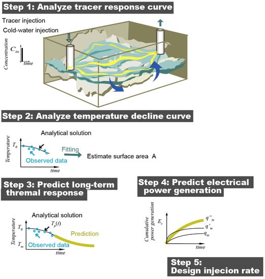
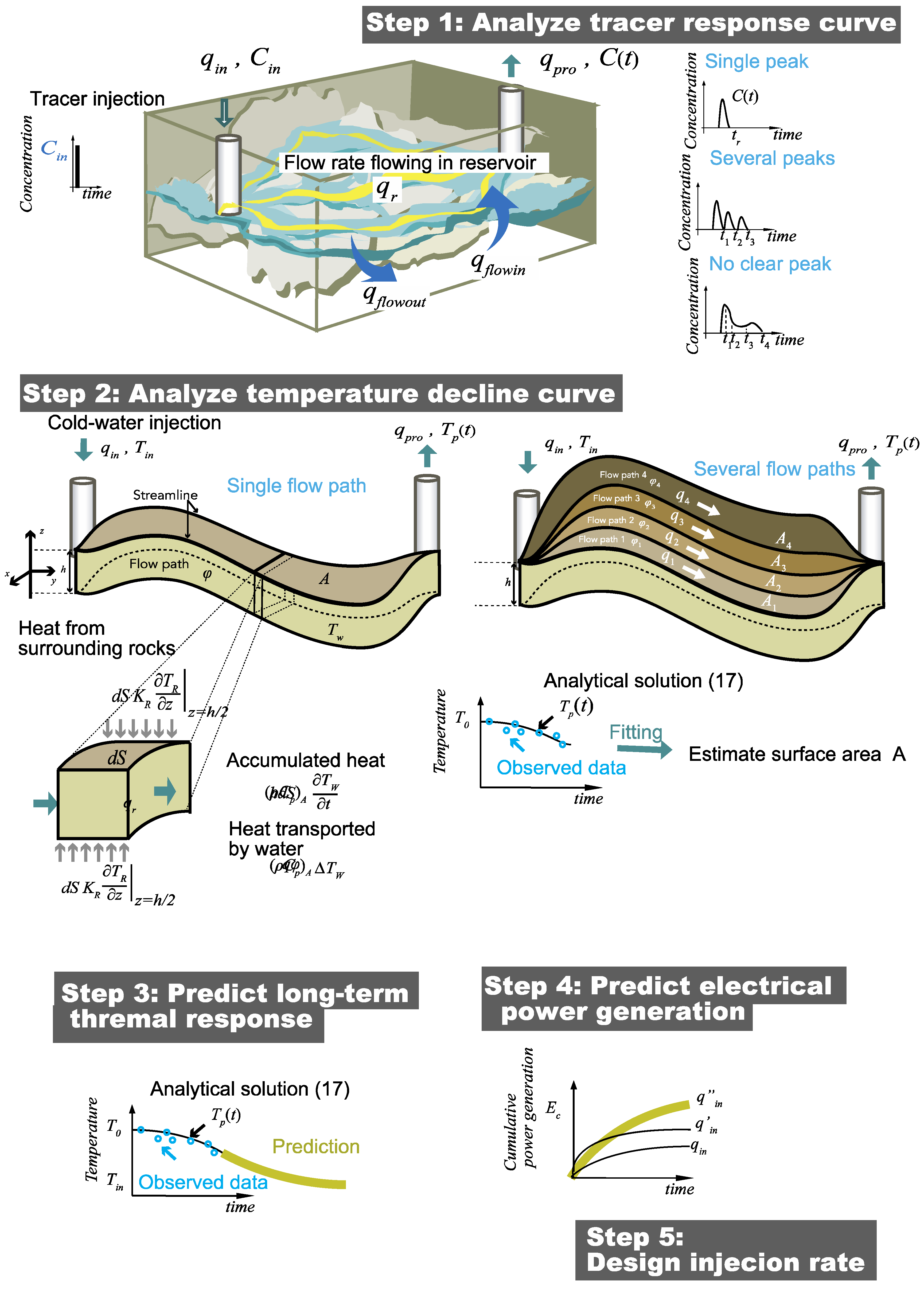
2. Methods
3. Validation
3.1. Simulation Setup
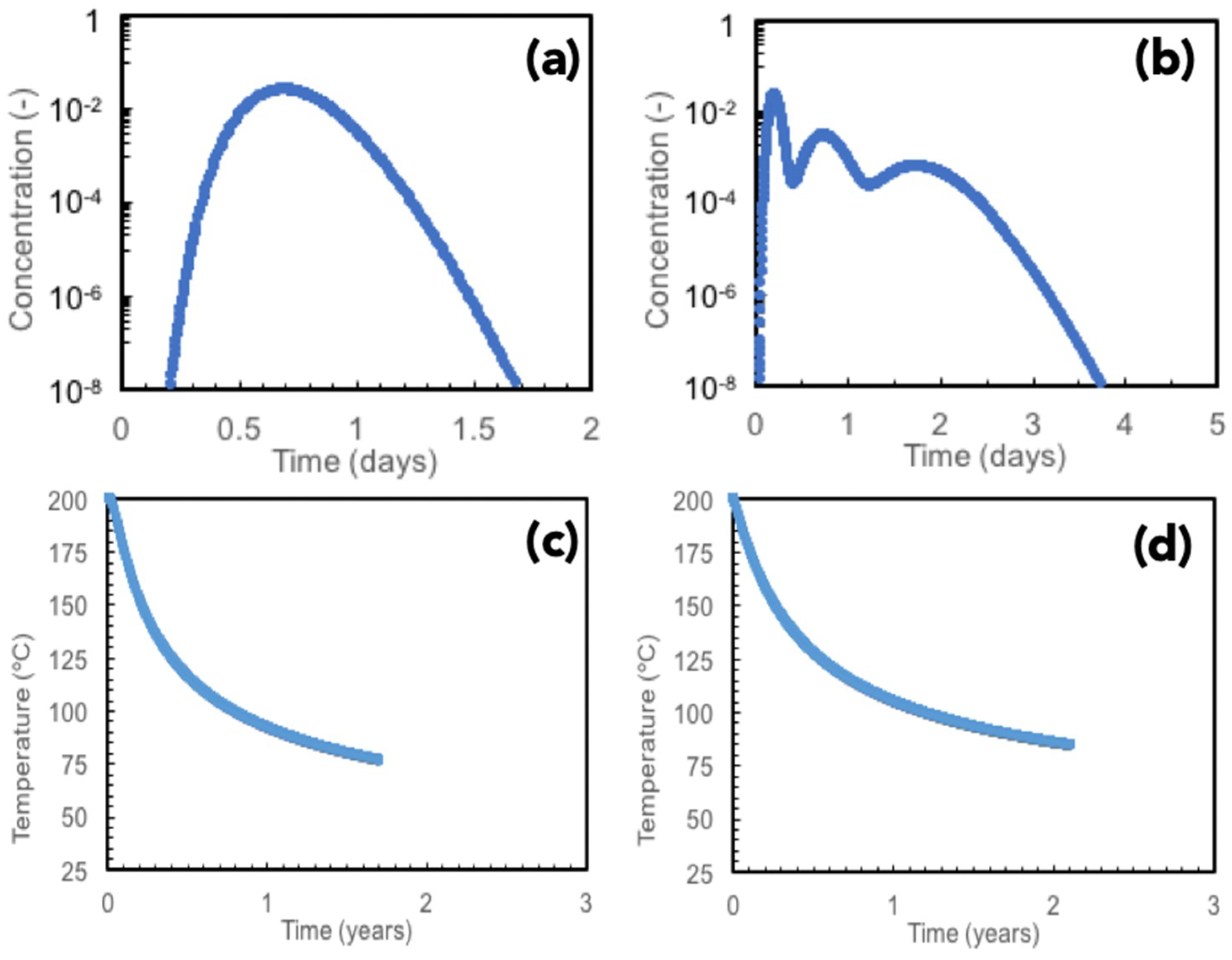
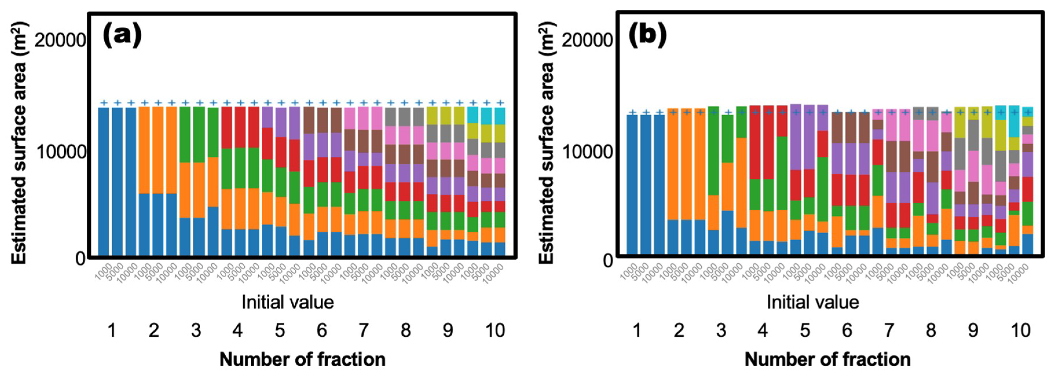
3.2. Numerical Results
4. Field Data
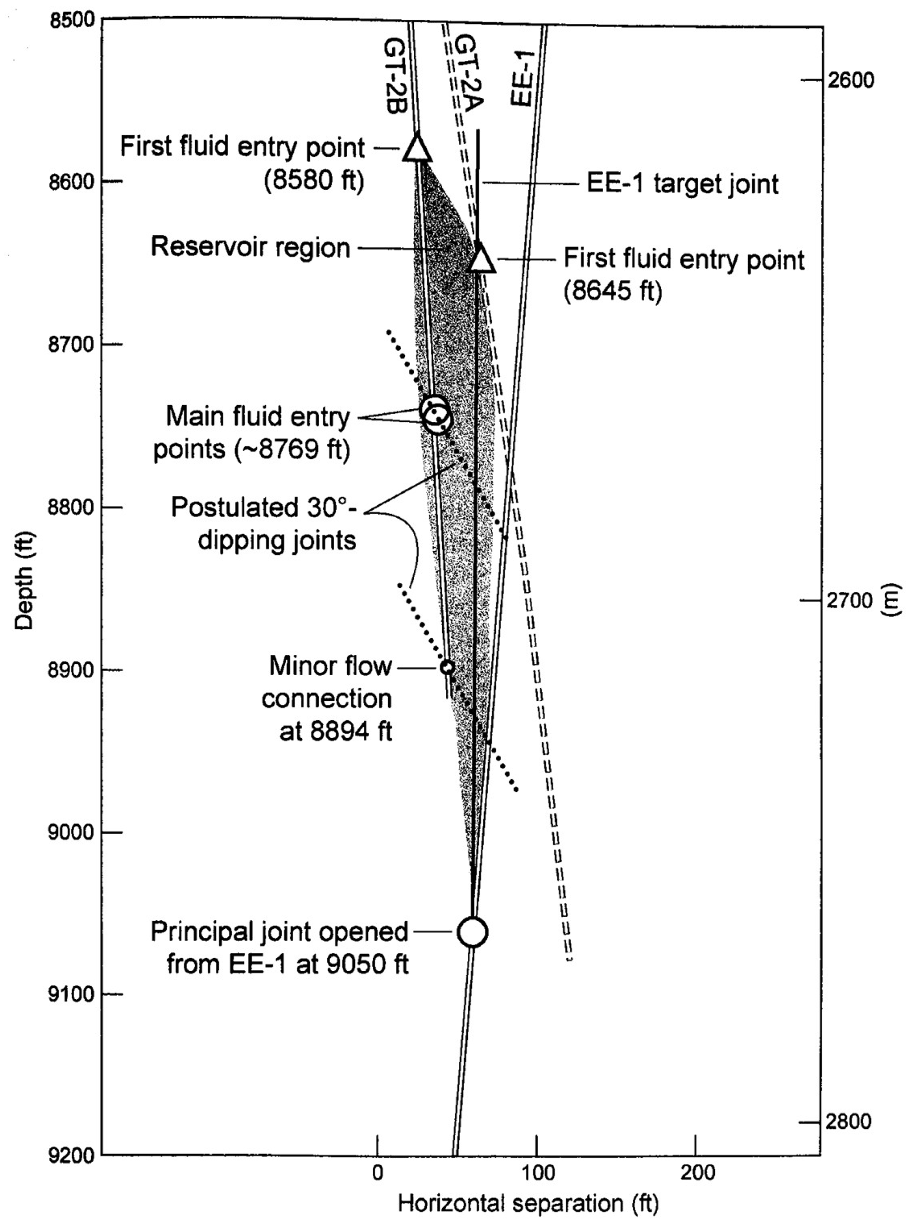
4.1. Fenton Hill Phase I Reservoir
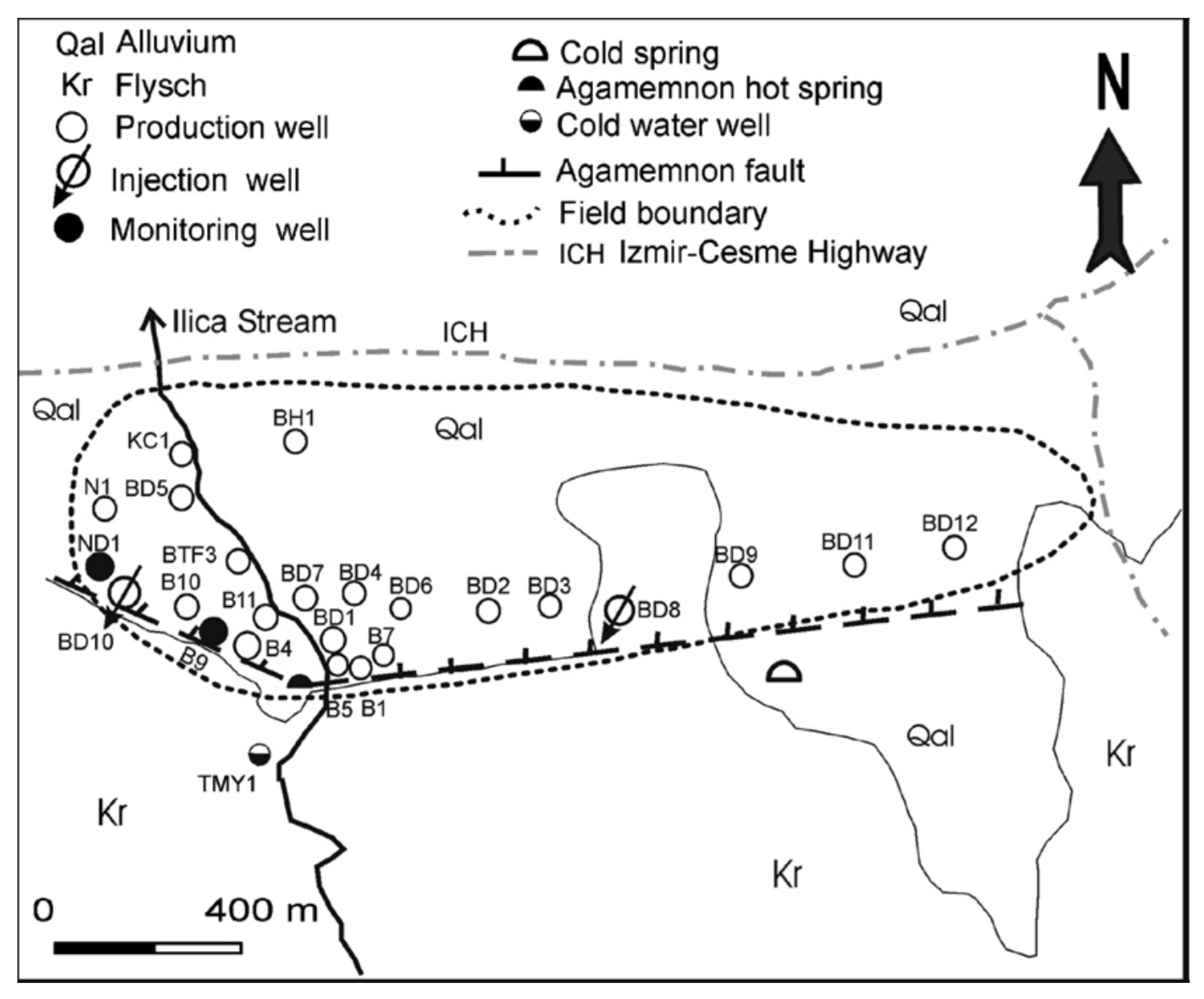
4.2. Balcova Geothermal Field, Turkey
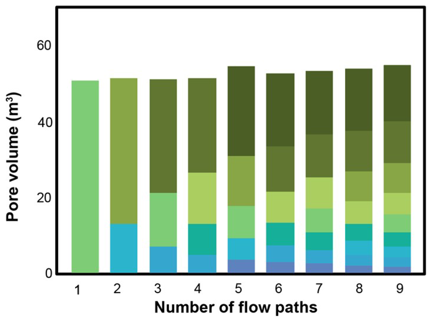
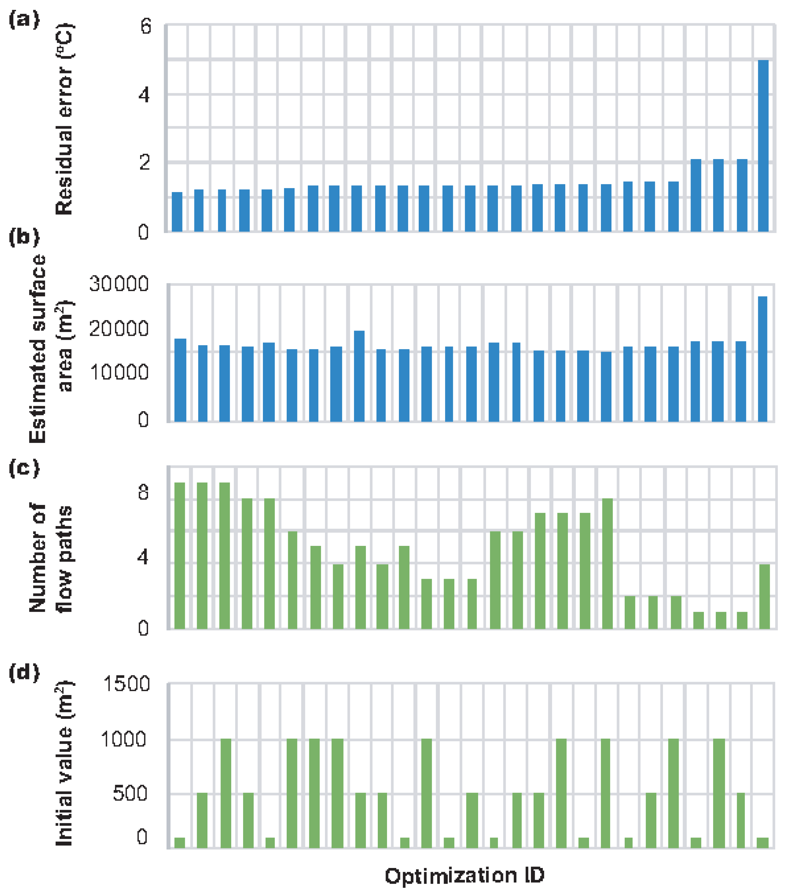
5. Results
5.1. Fenton Hill Geothermal Field, US
5.2. Balcova Geothermal Field, Turkey
5.3. Future Prediction
6. Discussion and Conclusions
Author Contributions
Funding
Acknowledgments
Conflicts of Interest
References
- Diersch, H.G. FEFLOW Finite-Element Subsurface Flow and Transport Simulation System. In User’s Manual⁄Reference Manual⁄White Papers; Release 5.4; WASY: Berlin, Germany, 2002. [Google Scholar] [CrossRef]
- Pruess, K.; Oldenburg, C.; Moridis, G. TOUGH2 User’s Guide, version 2.0; Earth Sciences Division, Lawrence Berkeley National Laboratory; University of California: Berkeley, CA, USA, 1999. [Google Scholar]
- Pruess, K.; Narasimhan, T.N. A Practical Method for Modeling Fluid and Heat Flow in Fractured Porous Media. SPE J. 1985, 25, 14–26. [Google Scholar] [CrossRef]
- Cacas, M.C.; Ledoux, E.; de Marsily, G.; Tillie, B.; Barbreau, A.; Durand, E.; Feuga, B.; Peaudecerf, P. Modeling fracture flow with a stochastic discrete fracture network: Calibration and validation: 1. The flow model. Water Resour. Res. 1990, 26, 479–489. [Google Scholar] [CrossRef]
- Lichtner, P.G.; Hammond, C.; Lu, S.; Karra, G.; Bisht, B.; Andre, R.M.; Kumar, J. PFLOTRAN User Manual: A Massively Parallel Reactive Flow and Transport Model for Describing Surface and Subsurface Processes; Technical Report L A-UR-15-20403; Los Alamos Natl. Lab.: Los Alamos, NM, USA, 2015. [Google Scholar]
- Painter, S.L.; Gable, C.W.; Kelkar, S. Pathline tracing on fully unstructured control-volume grids. Comput. Geosci. 2012, 16, 1125–1134. [Google Scholar] [CrossRef]
- Neuman, S.P. Trends, prospects and challenges in quantifying flow and transport through fractured rocks. Hydrogeol. J. 2005, 13, 124–147. [Google Scholar] [CrossRef]
- Shook, G.; Forsmann, J. Tracer Interpretation Using Temporal Moments on a Spreadsheet; Idaho Natl. Lab. (INL/EXT-05-00400), Ida-ho National Laboratory: Idaho Falls, ID, USA, 2005. [Google Scholar]
- Robinson, B.A.; Tester, J.W. Dispersed fluid flow in fractured reservoirs: An analysis of tracer-determined residence time distributions. J. Geophys. Res. Space Phys. 1984, 89, 10374–10384. [Google Scholar] [CrossRef]
- Robinson, B.A.; Tester, J.W.; Brown, L.F. Reservoir Sizing Using Inert and Chemically Reacting Tracers. SPE Form. Eval. 1988, 3, 227–234. [Google Scholar] [CrossRef]
- Pruess, K.; Bodvarsson, G. Thermal Effects of Reinjection in Geothermal Reservoirs With Major Vertical Fractures. J. Pet. Technol. 1984, 36, 1567–1578. [Google Scholar] [CrossRef]
- Horne, R.N.; Rodriguez, F. Dispersion in tracer flow in fractured geothermal systems. In Proceedings of the Seventh Workshop on Geothermal Engineering, Stanford University, Stanford, CA, USA, 15–17 December 1981; pp. 103–113. [Google Scholar]
- Walkup, G.; Horne, R.N. Characterization of tracer retention processes and their effect on tracer trans- port in fractured geothermal reservoirs. SPE paper #13610. In Proceedings of the SPE California Regional Meeting, Bakersfield, CA, USA, 27–29 March 1985. [Google Scholar]
- Arason, P.; Bjornsson, G. ICEBOX, 2nd ed.; Orkustofnun: Reykjavik, Iceland, 1994. [Google Scholar]
- Axelsson, G.; Bjomsson, G.; Fldvenz, O.G.; Kristmannsddttir, G.; Svemsddttir, G. Injection experiments in low-temperature geothermal areas in Iceland. In Proceedings of the World Geothermal Congress 1995, Florence, Italy, 18–31 May 1995; Available online: https://www.geothermal-energy.org/pdf/IGAstandard/WGC/1995/3-axelsson.pdf (accessed on 25 September 2019).
- Shook, G.M.; Suzuki, A. Use of tracers and temperature to estimate fracture surface area for EGS reservoirs. Geothermics 2017, 67, 40–47. [Google Scholar] [CrossRef]
- Ikhwanda, F.; Suzuki, A.; Willis-Richards, J.; Hashida, T. 122 Development of Numerical Methods for Estimating Fluid Flow Path in Fractured Geothermal Reservoir. Proc. Conf. Tohoku Branch 2018, 43–44. [Google Scholar] [CrossRef][Green Version]
- Gringarten, A.C.; Sauty, J.P. A theoretical study of heat extraction from aquifers with uniform regional flow. J. Geophys. Res. Space Phys. 1975, 80, 4956–4962. [Google Scholar] [CrossRef]
- Moon, H.; Zarrouk, S.J. Efficiency of geothermal power plants: A worldwide review. In Proceedings of the 2012 New Zealand Geothermal Workshop, Auckland, New Zealand, 19–21 November 2012; Available online: http://www.geothermal-energy.org/pdf/IGAstandard/NZGW/2012/46654final00097.pdf (accessed on 6 September 2019).
- Pruess, K.; Moridis, G. Tough 2 User’s Guide, version 2; Lawrence Berkeley National Laboratory: Berkeley, CA, USA, 2011; LBNL-43134. [Google Scholar]
- Dash, Z.V.; Murphy, H.D.; Aamodt, R.L.; Aguilar, R.G.; Brown, D.W.; Counce, D.A.; Fisher, H.N.; Grigsby, C.O.; Keppler, H.; Laughlin, A.W.; et al. Hot dry rock geothermal reservoir testing: 1978 to 1980. Volcanol. Geotherm. Res. 1983, 15, 59–99. [Google Scholar] [CrossRef]
- Brown, D.W.; Duchane, D.V.; Heiken, G.; Hriscu, V.T. Mining the Earth’s Heat: Hot Dry Rock Geothermal Energy; Springer Science & Business Media: Berlin, Germany, 2012. [Google Scholar] [CrossRef]
- Tester, J.W.; Albright, J.N. Hot Dry Rock Energy Extraction Field Test: 75 Days of Operation of a Prototype Reservoir at Fenton Hill Segment 2 of Phase I; Los Alamos Scientific Laboratory Report LA-7771-MS.; Los Alamos Natl. Lab.: Los Alamos, NM, USA, April 1979. [Google Scholar] [CrossRef][Green Version]
- Aksoy, N.; Serpen, U.; Şevki, F. Management of the Balcova–Narlidere geothermal reservoir, Turkey. Geothermics 2008, 37, 444–466. [Google Scholar] [CrossRef]
- Arkan, S.; Parlaktuna, M. Resource Assessment of Balçova Geothermal Field. In Proceedings of the World Geothermal Congress 2005, Anatalya, Turkey, 24–29 April 2005; Available online: https://www.geothermal-energy.org/pdf/IGAstandard/WGC/2005/1130.pdf (accessed on 9 September 2019).
- Shook, G. Predicting thermal breakthrough in heterogeneous media from tracer tests. Geothermics 2001, 30, 573–589. [Google Scholar] [CrossRef]
- Wu, X.; Pope, G.A.; Shook, G.M.; Srinivasan, S. Prediction of enthalpy production from fractured geothermal reservoirs using partitioning tracers. Int. J. Heat Mass Transf. 2008, 51, 1453–1466. [Google Scholar] [CrossRef]
- Axelsson, G.; Flovenz, O.G.; Hauksdottir, S.; Hjartarson, A.; Liu, J. Analysis of tracer test data, and injection-induced cooling, in the Laugaland geothermal field, N-Iceland. Geothermics 2001, 30, 697–725. [Google Scholar] [CrossRef]
- Stefansson, V. Gehermal reinjection experience. Geothermics 1997, 26, 99–139. [Google Scholar] [CrossRef]
- Kocabas, I.; Horne, R.N. A new method offorecasting the thermal breakthrough time during reinjection in geothermal reservoirs. In Proceedings of the 15th Workshop on Geothermal Reservoir Engineering 1990, Stanford University, Stanford, CA, USA, 23–25 January 1990; pp. 179–186. [Google Scholar]
- Kocabas, I. Geothermal reservoir characterization via thermal injection back-flow and interwell tracer testing. Geothermics 2005, 34, 27–46. [Google Scholar] [CrossRef]
- Adams, M.C.; Davis, J. Kinetics of fluorescein decay and its application as a geothermal tracer. Geothermics 1991, 20, 53–66. [Google Scholar] [CrossRef]
- Hawkins, A.J.; Becker, M.W.; Tsoflias, G.P. Evaluation of inert tracers in a bedrock fracture using ground penetrating radar and thermal sensors. Geothermics 2017, 67, 86–94. [Google Scholar] [CrossRef]
- Müller, K.; VanderBorght, J.; Englert, A.; Kemna, A.; Huisman, J.A.; Rings, J.; Vereecken, H. Imaging and characterization of solute transport during two tracer tests in a shallow aquifer using electrical resistivity tomography and multilevel groundwater samplers. Water Resour. Res. 2010, 46, W03502. [Google Scholar] [CrossRef]
- Hermans, T.; Vandenbohede, A.; Lebbe, L.; Nguyen, F. A shallow geothermal experiment in a sandy aquifer monitored using electric resistivity tomography. Geophysics 2012, 77, B11–B21. [Google Scholar] [CrossRef]


| Parameter | Value | Parameter | Value | ||
|---|---|---|---|---|---|
| Rock Density (kg/m3) | 2569 | Single fracture | Three flow paths | ||
| Rock heat capacity (J/kg °C) | 803 | Porosity (-) | 0.9 | DZ 1 | 0.75 |
| Rock thermal conductivity (W/m °C) | 2.569 | Fracture | 0.5 | ||
| Water density at 25 °C (kg/m3) | 997.1 | DZ 2 | 0.95 | ||
| Water density at 200 °C (kg/m3) | 864 | Permeability (10−12 m2) | 10 | DZ 1 | 4 |
| Water heat capacity at 25 °C (J/kg K) | 4180 | Fracture | 10 | ||
| Thermal conductivity at 200 °C (J/kg K) | 4510 | DZ 2 | 2 | ||
| Initial pressure (kPa) | 9800 | Pore volume (m3) | 125.55 | DZ 1 | 34.875 |
| Initial temperature (°C) | 200 | Fracture | 23.25 | ||
| Flow rate (kg/s) | 2 | DZ 2 | 44.175 | ||
| Injection temperature (°C) | 25 | A (m2) | 13,950 | DZ 1 | 4650 |
| Model dimensions (m) | 99 × 75 × 643 | Fracture | 4650 | ||
| Grid dimensions | 33 × 15 × 3 | DZ 2 | 4650 | ||
| ΔX (m) | 3 | ||||
| ΔY (m) | 0.01, 0.02, 0.04, … | ||||
| ΔZ (m) | 25 | ||||
| Parameter | Most Likely | Min | Max |
|---|---|---|---|
| Porosity [-] | - | 0.002 | 0.070 |
| Rock specific heat [J/kg] | 0.92 | 0.80 | 1.08 |
| Rock density [kg/m3] | 2750 | 2600 | 2850 |
| Rock temperature [°C] | 135 | 100 | 145 |
| Area [m2] | 9.00 × 10⁵ | 5. 00 × 105 | 2. 00 × 105 |
| Thickness [km] | 0.35 | 0.25 | 1.00 |
| Fluid density [kg/m3] | 930.6 | 921.7 | 958.1 |
| Utilized temperature [°C] | 80 | - | - |
| Fluid specific heat [J/kg] | 4.18 | - | - |
© 2019 by the authors. Licensee MDPI, Basel, Switzerland. This article is an open access article distributed under the terms and conditions of the Creative Commons Attribution (CC BY) license (http://creativecommons.org/licenses/by/4.0/).
Share and Cite
Suzuki, A.; Ikhwanda, F.; Yamaguchi, A.; Hashida, T. Estimations of Fracture Surface Area Using Tracer and Temperature Data in Geothermal Fields. Geosciences 2019, 9, 425. https://doi.org/10.3390/geosciences9100425
Suzuki A, Ikhwanda F, Yamaguchi A, Hashida T. Estimations of Fracture Surface Area Using Tracer and Temperature Data in Geothermal Fields. Geosciences. 2019; 9(10):425. https://doi.org/10.3390/geosciences9100425
Chicago/Turabian StyleSuzuki, Anna, Fuad Ikhwanda, Aoi Yamaguchi, and Toshiyuki Hashida. 2019. "Estimations of Fracture Surface Area Using Tracer and Temperature Data in Geothermal Fields" Geosciences 9, no. 10: 425. https://doi.org/10.3390/geosciences9100425
APA StyleSuzuki, A., Ikhwanda, F., Yamaguchi, A., & Hashida, T. (2019). Estimations of Fracture Surface Area Using Tracer and Temperature Data in Geothermal Fields. Geosciences, 9(10), 425. https://doi.org/10.3390/geosciences9100425