Article

Constrained Full Waveform Inversion for Borehole Multicomponent Seismic Data

by
Marwan Charara
1,* and
Christophe Barnes
2
1
Skolkovo Institute of Science and Technology, Moscow 121205, Russia
2
Department of Geosciences and Environment, University of Cergy-Pontoise, 95000 Neuville-sur-Oise, France
*
Author to whom correspondence should be addressed.
Geosciences 2019, 9(1), 45; https://doi.org/10.3390/geosciences9010045
Submission received: 2 December 2018 / Revised: 25 December 2018 / Accepted: 25 December 2018 / Published: 16 January 2019
(This article belongs to the Special Issue Numerical Methods of Geophysical Fields Inversion)

Abstract

:
Full-waveform inversion for borehole seismic data is an ill-posed problem and constraining the problem is crucial. Constraints can be imposed on the data and model space through covariance matrices. Usually, they are set to a diagonal matrix. For the data space, signal polarization information can be used to evaluate the data uncertainties. The inversion forces the synthetic data to fit the polarization of observed data. A synthetic inversion for a 2D-2C data estimating a 1D elastic model shows a clear improvement, especially at the level of the receivers. For the model space, horizontal and vertical spatial correlations using a Laplace distribution can be used to fill the model space covariance matrix. This approach reduces the degree of freedom of the inverse problem, which can be quantitatively evaluated. Strong horizontal spatial correlation distances favor a tabular geological model whenever it does not contradict the data. The relaxation of the spatial correlation distances from large to small during the iterative inversion process allows the recovery of geological objects of the same size, which regularizes the inverse problem. Synthetic constrained and unconstrained inversions for 2D-2C crosswell data show the clear improvement of the inversion results when constraints are used.

1. Introduction

Full-waveform inversion of seismic data allows one to obtain an image of the subsurface through the determination of a certain number of physical parameters. Borehole data (VSP and crosswell) are of special interest because of the geometry of acquisition, which provides more informative signals on the medium properties than surface seismic data (high frequency signal, energetic P-S conversions). However, the lack of seismic data redundancy (e.g., few shots) renders the inversion problem underdetermined. In general, full-waveform inversion is an ill-posed problem, in the sense that an infinite number of models match the data [1]. It is classically solved with local optimization schemes and is therefore strongly dependent on the starting model definition. This starting model should predict arrival times with errors less than half of the period to cancel the cycle-skipping ambiguity [1]. The multiscale strategy performed by moving from low to high frequencies during the inversion allows reduction of the nonlinearities and cycle skipping issues of the inversion and helps convergence toward the global minimum. Regularizations are conventionally applied to the inversion in the model space to make it better posed [2,3]. Tikhonov and Arsenin [4] have proposed a regularization strategy within the optimization step to find the smoothest model that explains the data. Preconditioning techniques acting as a smooth operator on the model update [5] may add strong prior features of the expected structure through directive Laplace preconditioning, as in Guitton et al. [6]. Regularization schemes that preserve edges and contrasts have also been developed for specific full waveform inversion applications through a 1 model penalty [7] or through a multiplicative regularization [8]. Regularization can also be expressed in the curvelet or wavelet domains [9,10]. In such domains, the 1 norm minimization is generally preferred for the model term penalty because it ensures sparsity in the model space. All the previous regularization techniques allow stabilization of the inversion scheme by assuming a particular representation or structure of the velocity model (smoothness, sparsity, and so on). However, geological information, taking into account prior model information, is generally not used in classical full waveform inversion implementation; however, there are some examples [11,12]. In addition, most of the weighting operators or covariance matrices associated with the model parameters are set to identity or in the best cases to a diagonal matrix. The same applies to the weighting operators or covariance matrices associated with the data.
Weighting operators on the data and models or inverse of the data and model covariance operators for least squares in the frame of the Bayesian formulation [3] are introduced in the misfit function. In this paper, we will show the benefit of introducing covariance matrices in the data and model space. On the one hand, we will illustrate the impact on constraining the seismic inverse problem on the data space for the case of a synthetic two-component borehole seismic data by using the polarization analysis to fill a block diagonal data space covariance matrix. On the other hand, we will illustrate the benefit of constraining the seismic inverse problem on the model space by performing a crosswell synthetic experiment. The horizontal and vertical spatial correlations using Laplace distribution are used to fill the model space covariance matrix in order to introduce an a priori solution, favoring a tabular medium whenever it doesn’t contradict the information contained in the data.

2. Constrained Least Squares Inversion

Using the probabilistic formalism developed by Tarantola [3] and considering only the data space term in the equation, we rewrite the misfit function in the vicinity of the current model m n :
S ( m n + δ m ) = ( δ d n G n δ m ) T C D 1 ( δ d n G n δ m ) + ( Δ m n δ m ) T C M 1 ( Δ m n δ m ) ,
where:
  • δ m is the perturbation in the vicinity of the current model m n ,
  • δ d n are the data residuals for the model m n ,
  • Δ m n is the difference between the current model m n and the a priori model m p r i o r
  • G n is the linear function tangent to g at the model m n ,
  • g is the function mapping the model space m M into the data space d = g ( m ) D
  • C D is the covariance matrix on the data space.
  • C M is the covariance matrix on the model space (defining the Gaussian a priori probability density).
Applied to the waveform inversion problem of estimating the elastic parameters and the density of the earth, the minimization of the misfit function can be solved by iterative gradient methods.
The iterative process of a nonlinear inversion can be summarized as follows [3]: for a given iteration k , from the current model m k (i.e., the discretized physical fields characterizing the medium), we perform simulations of the wave in order to obtain the synthetic data   d k c a l = g ( m k ) . Thus, comparing them to observed data   d o b s , we obtain the residuals   δ d k = d o b s   d k c a l . These residuals are weighted   δ d ^ k = C D 1 δ d k (the hat denotes the dual space) and back-propagated using the wave propagation equation again to obtain the gradient in the dual model space   γ ^ k =   G k T C D 1 δ d k (where G k is the derivative of the function g over the model space at the point m k and where   T denotes the transpose operation) and consequently, the gradient in the model space   γ k = C M γ ^ k . The gradient indicates the steepest ascent direction of the misfit function in the model space. We modify this direction using the conjugate gradient algorithm   φ k = γ k +   α k φ k 1 , where φ k is the conjugate gradient and α k is defined from the gradient [13]. Finally, using an additional simulation, we optimize the step length μ k [14] in the upgrading equation m k + 1 = m k μ k φ k and we update the model.

3. Constraints on the Data Space

The quantification of uncertainties in seismic data is often neglected, because in many cases it is a difficult task. For instance, data errors generated by receiver response are correlated in time, which means accounting for them is not straightforward. To illustrate the possible contribution of constraints provided by the analysis of uncertainties of data, we have performed two inversions from the synthetic data experiment. The first inversion is done without any data constraints, whereas in the second one we have incorporated polarization wave analysis in the covariance matrix C D . This matrix treats the uncertainties on particle velocities according to the eigenbasis of the particle motion.
For the case of multi-component data, the uncertainty of a component may be correlated to the uncertainty of the other components. For each time for each of the receiver components, we can define a 2 × 2 matrix for 2-component data (as in the example bellow), or a 3 × 3 matrix for 3-component data. In that case, the covariance matrix on the data space C D is not a diagonal matrix. In order to take into account polarization, we consider that the uncertainties are proportional to the local cross-correlation matrix of the signal (the data) and that the signal is locally stationary (over 2 periods). The cross-correlation matrix between components i and j of the signal s r , t is computed with zero lag ( τ = 0 ) for any receiver r and any time t :
C r , t i j ( τ ) = + s r , t i ( u ) s r , t j ( u + τ ) d u ,
where:
s r , t i ( u ) = d r i ( u )   w t ( u )
with d r i ( u ) being the trace for the component i of the receiver r of the observed data and w t ( u ) a Hamming time window centered on time t with a length of typically 2 periods. One can use other time tapering windows classically used in spectral analysis (Blackman, Nuttall, etc).

3.1. Cross-Correlations and Polarization

The polarization of the multicomponent signal is estimated from this matrix C r , t i j ( τ = 0 ) and the matrix of the uncertainties has the same eigenvectors (polarization directions) than the cross-correlation matrix. The uncertainty has the same shape as the polarization of the signal. The ratios among the eigenvalues are the same, in other words, the rectilinearity and planarity of the polarization [15] is conserved.
The polarized signal for rectilinear polarization can be modeled by:
d ( t ) = a · s ( t ) + n ( t ) ,
where d ( t ) is the 3C signal, a is the polarization vector,   s ( t ) the scalar signal along the polarization vector, and n ( t ) the 3C Gaussian noise.
In the frequency domain, the equation can be expressed as:
d ^ ( f ) = a · s ^ ( f ) + n ^ ( f ) ,
where the hat denotes the frequency domain.
Let us consider the spectral matrix of the 3C signal defined by:
S ^ ( f ) = d ^ ¯ ( f ) · d ^ T ( f ) = ( a s ^ + n ^ ) ¯ · ( a s ^ + n ^ ) T = a · a T · s ^ ¯ s ^ + n ^ ¯ · n ^ T = a · a T | s ^ ( f ) | 2 + N ^ ( f ) ,
where the upper bar denotes the complex conjugate, T denotes the transpose operator and N ^ ( f ) being the spectral matrix of the noise. Note that ( a s ^ ) ¯ · n ^ T = n ^ ¯ · a T s ^ = 0 because noise and signal are considered uncorrelated. The polarization vector is an eigenvector of the spectral matrix (for isotropic noise) for any frequency   f :
S ^ · a = ( a · a T | s ^ | 2 + N ^ ) a = | s ^ | 2 a · a T a + N ^ a = | s ^ | 2 a + ( | n ^ | 2 I ) a = ( | s ^ | 2 + | n ^ | 2 ) a .
When integrating the spectral matrix over , one obtains the cross-correlation matrix C ( τ = 0 )   with zero lag with the same eigenvectors.
The structure of the covariance matrix on the data space C D is derived from the previous equations. For instance, for a 2C receiver, a given source or receiver couple, and at any time t , the corresponding 2 × 2 submatrix is defined as:
C D = V · σ D 2 ( 1 0 0 λ II λ I ) · V 1
where V is the eigenvectors matrix (column), σ D is the standard deviation of the (isotropic) noise for this couple, and λ I and λ II are the max and min of the two positive eigenvalues of the spectral matrix, respectively.
Let us consider the sub-matrix for the first data 2C-trace of the covariance matrix on the data space:
C D ( r e c = 1 ) C D ( r = 1 , t , τ = 0 )
[ σ 1 , X 2 ρ 1 σ 1 , X σ 1 , Z 0 0 0 0 0 ρ 1 σ 1 , X σ 1 , Z σ 1 , Z 2 0 0 0 0 0 0 σ 2 , X 2 ρ 2 σ 2 , X σ 2 , Z 0 0 0 0 ρ 2 σ 2 , X σ 2 , Z σ 2 , Z 2 0 0 0 0 0 0 σ n t , Z 2 ρ n t σ n t , X σ n t , Z 0 0 0 0 ρ n t σ n t , X σ n t , Z σ n t , Z 2 ]
where ρ i , σ i , X , and σ i , Z are, respectively, the correlation coefficient, the standard deviation for the X component, and the standard deviation for the Z component for a given time sample i , and n t being the total number of time samples. The matrix C D is a block diagonal matrix and its inverse (i.e.,   C D 1 , is another block diagonal matrix), composed of the inverse of each block.

3.2. An Offset VSP Synthetic Example

In this numerical example, the acquisition geometry is an offset VSP with a unique source at 500 m offset and the antenna is between 580 and 970 m depth in a vertical well (see Figure 1 for more details). The isotropic elastic model depends only on the depth (1D model). The “true” model is defined in Figure 1. The horizontal and vertical components of the “observed” data obtained from the true model are displayed in Figure 1. The direct problem (seismic modeling) is based on discretizing the wave equation by the finite differences method (FDM) [16].
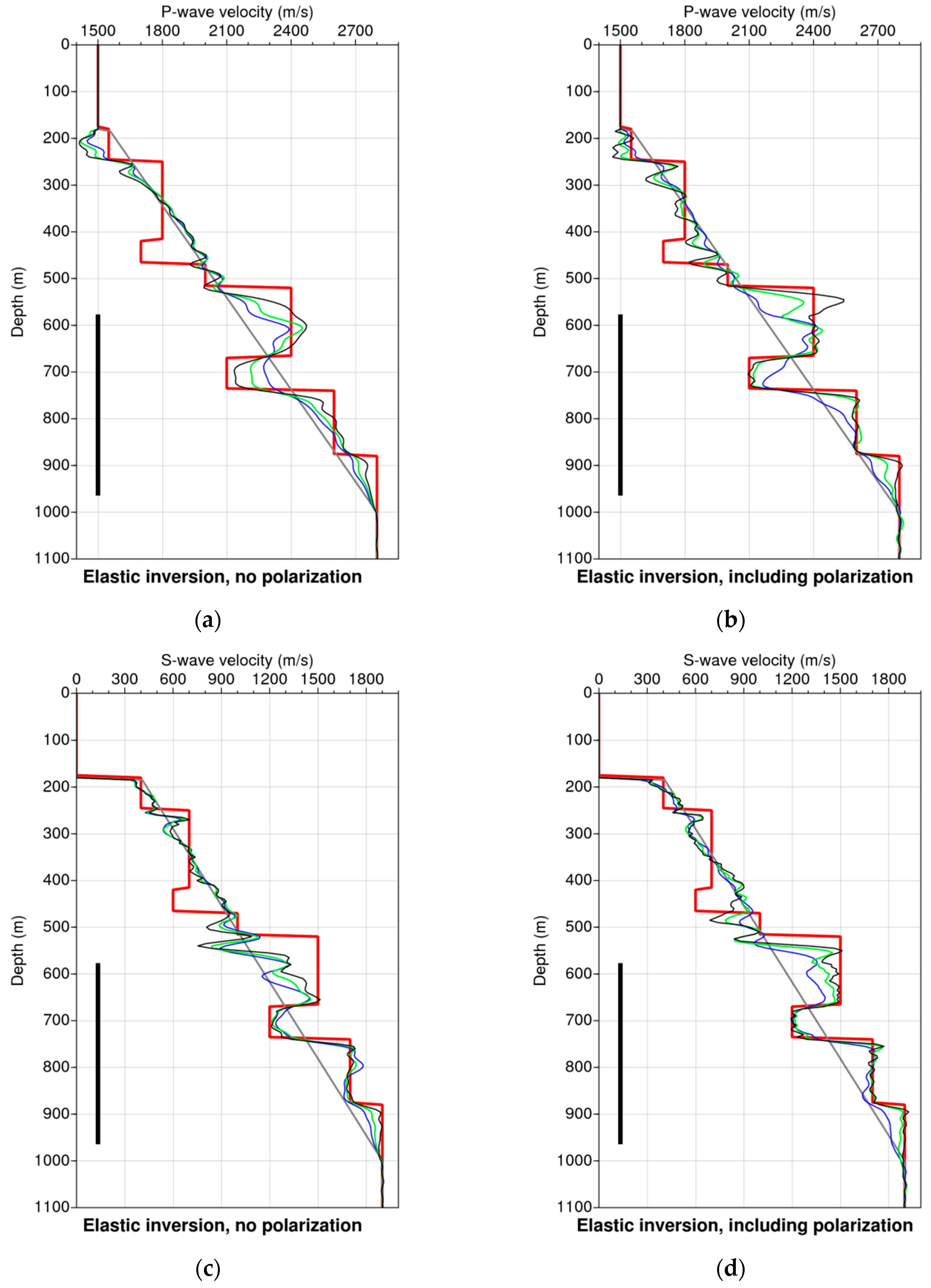
The inverted parameters are the P-wave velocity, the S-wave velocity, and the density. The starting models are simple, the water layer is considered as known, and the other layers are replaced by a constant vertical gradient for each parameter (gray solid lines in Figure 2). The test consists of comparing the results of inversion when data uncertainties are isotropic and when the polarization is included in the data uncertainties.
As shown in Figure 2, the inversion results exhibits in both cases a good fit in the receiver zone, while the estimation is not good in the upper part of the model. One can clearly note that the S-wave velocity model is recovered with more detail than the P-wave velocity model. This is due to the fact that converted S-waves are present in borehole seismic data and also because the S-waves have a shorter wavelength than P-waves, hence, a better spatial resolution. The final residuals for both inversion experiments are small; a few percent of the misfit. The inversion results when polarization is included are significantly better than for the isotropic uncertainties. More precisely, for the case of polarization, both P-wave and S-wave estimated velocity fields are well fitted in the antenna zone.

4. Constraints on the Model Space

We can distinguish two kinds of geological a priori information that can be incorporated in an inversion process. On the one hand, information obtained by measurements (well logging), that we consider as “objective” information, allows the definition of an a priori model at the well vicinity. On the other hand, information coming from geological interpretations, such as geological layer dips, that we qualify as “subjective” information, can be simplified and introduced into the covariance matrix C M .

4.1. Quantification of Number of Degrees of Freedom

In order to evaluate the importance of constraints on an inversion, it is necessary to quantify the number of degrees of freedom. This number can be estimated from the set of parameters as a function of existing correlations among them and independently of their standard deviations. The number N of free parameters is equal to the number n of parameters in the absence of correlations, and it is reduced to 1 in the case of perfect correlations.

4.1.1. General Case

Let us consider a 1D Gaussian random field X , the domain is discrete and finite consisting of a set of n points; this field is equivalent to the set of random variables ( X 1 ,   X 2 , , X n ) . It can be characterized by the following probability density function (or p.d.f.):
f ( x ) = 1 ( 2 π ) n / 2 det ( C ) 1 / 2 exp ( 1 2 ( x m ) T C 1 ( x m ) ) ,
where x is a realization, m is the expectation of the field ( E ( X ) = m ) , and C is the covariance matrix of the field.
The covariance matrix can be rewritten with the following form = S R S , where R is the correlation matrix and S the diagonal matrix of the standard deviations.
If there is no correlation among the random variables X i , then R = I and the covariance matrix is diagonal and the number of free parameters is then n . If a correlation exists, we then use the L U decomposition method to estimate the number of free parameters (see Appendix A and Appendix B for more details). We can write R = M M T where M is the left lower triangle matrix of the L U decomposition of the matrix R . The number of free parameters is then reduced to:
N = t r a c e ( M ) .

4.1.2. Spatial Correlation on the Model Space

For illustration purposes, let us consider the special case where the spatial correlations are described by an exponential model. Thus, for any pair of points M 1 and M 2 (belonging to the same horizontal line), the correlation ρ between the pair of random variables X 1 and X 2 corresponding to the points M i can be expressed as a function of the distance:
ρ ( X 1 , X 2 ) = exp ( d ( M 1 , M 2 ) r ) ,
where d ( · ) is a distance and r is the range of the correlation.
By setting the variance for each variable to be constant σ i = σ 1   , the p.d.f. of Equation (7) reduces to,
f ( x ) = 1 ( 2 π ) n / 2 · σ n det ( R ) exp ( 1 2 ( x m σ ) T R 1 ( x m σ ) ) ,
This simplifies, as we will show below, the study of the relation between the matrix R and the degrees of freedom using an exponential correlation function.
Let us consider the same Gaussian field X , but this time defined on a defined 1 D domain regularly sampled (as for a grid) containing n points. The distances between points are multiples of the step Δ x and the correlation matrix has the following form (for ordered points):
R = ( 1 a a 2 a 3 a 4 a n a 1 a a 2 a 3 a n 1 a n a n 1 a n 2 a n 3 a n 4 1 ) ,
where
a = exp ( Δ x   r ) 1 .
One interesting property of the R matrix is that the M matrix of the L U decomposition has a simple form
M = ( 1 0 0 0 0 0 a b 0 0 0 0 a 2 a b b 0 0 0 a n a n 1 b a n 2 b a n 3 b a n 4 b b ) ,
with   b = 1 a 2 . This means that, in terms of a sequential simulation, the   n 1 variables, X 2 to X n , have the same degree of freedom: b . The total degrees of freedom N of the field X is then:
N = 1 + ( n 1 ) · b ,
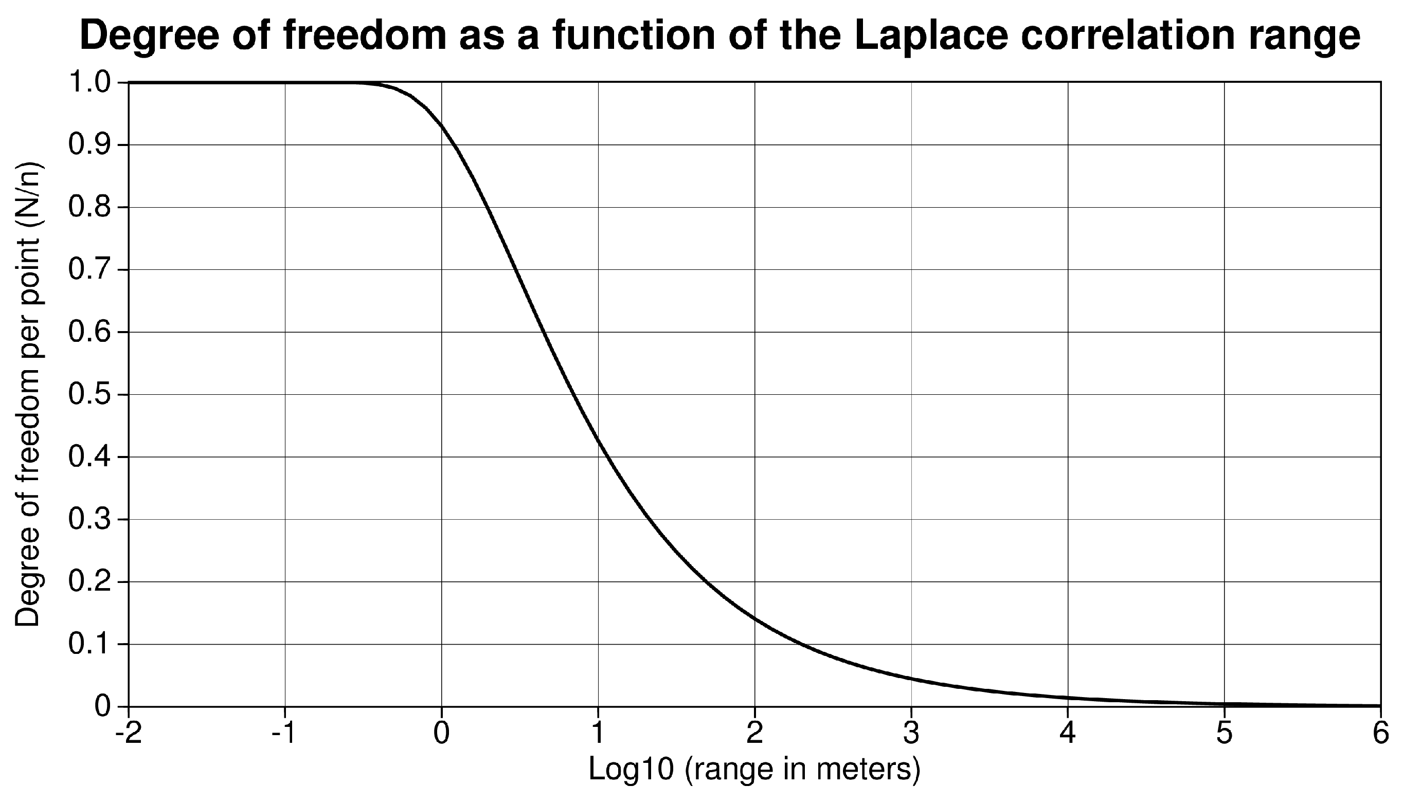
where for n parameters (or n grid points), the number of free parameters, considered as the degrees of freedom, of the inversion is N . Figure 3 shows the relation between the range of the correlation (expressed in number of steps, Δ x ) and the values of b .

4.2. Seismic Crosswell Numerical Experiment Example

This numerical example is an illustration how to incorporate the “subjective” geological information that our medium is mainly tabular but might contain complex geological structures using the covariance matrix on the model space.

4.2.1. Description of the Crosswell Experiment and Observed Data

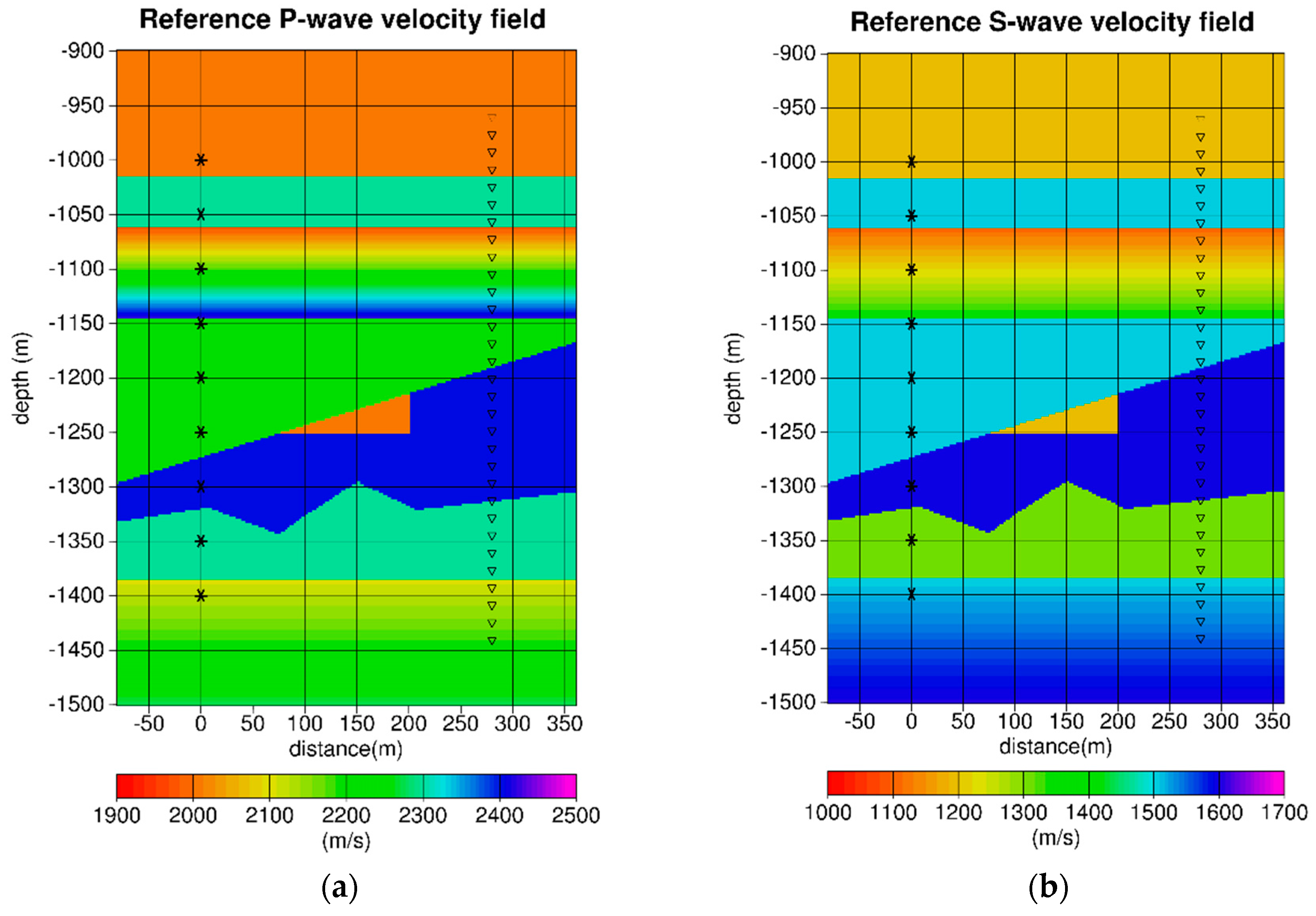
The reference subsurface models are shown in Figure 4. The word “reference” indicates that this model is used to generate the synthetic seismic data used as observed data (see Figure 5) during the inversion process. It is also the model to be retrieved by applying the full-wave inversion method to the observed data. The medium for wave propagation is elastic isotropic. The parameters to be inverted are discretized physical fields: vertical P-wave and S-wave velocities. For simplicity, the density ( ρ ) is not inverted—the field is constant with ρ = 2500   kg · m 3 and it fixed at the correct value in the different inversions.

4.2.2. Multiscale Constrained Inversion

The inversion process consists of four successive inversions using the same observed data but with decreasing correlation ranges in horizontal and vertical directions; therefore, it is a multiscale inversion and each inversion is for a given “scale”. The model parameter results of each inversion are used as initial model parameters for the next inversion.
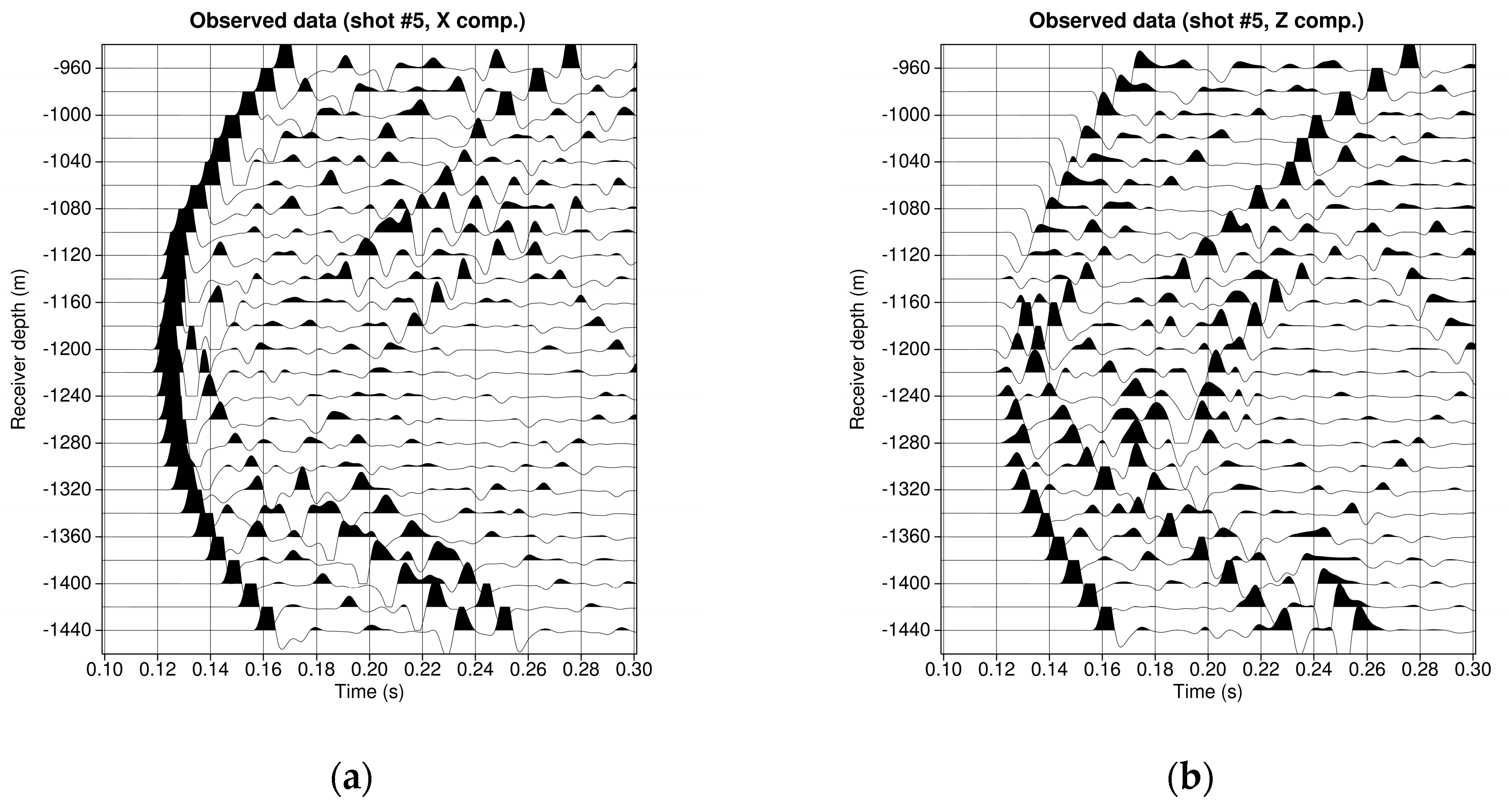
Uncertainties on the model space are required for the definition of C M 1 . It can be defined by specifying the spatial correlation ranges and the uncertainties on the parameters. Here the uncertainties on the parameters are kept constant: σ V p = 120   m / s and σ V s = 100   m / s . The ranges of the horizontal and vertical correlations do not depend on the parameters but on the spatial location. The horizontal correlation depends on depth and both horizontal and vertical ranges depend on the inversion scale. We define three types of a priori regions with respect to depth (see Table 1): “Quasi 1D” with large correlation ranges, “2D” with short correlation ranges (where we expect to have complex geological objects, see Figure 4), and “Transition”, with correlation ranges linearly varying with depth to match the ranges of the two adjacent regions.
Table 2 lists the different correlation ranges associated with the four successive inversion scales and for the a priori region types. The four successive inversion scales are denoted by (b), (c), (d), and (e) in relation to the results displayed in Figure 6 and Figure 7. The correlation ranges are gradually decreasing with the successive inversion scales in order to solve first the large wavelengths in the model before resolving the small wavelengths (i.e., the small model structures).
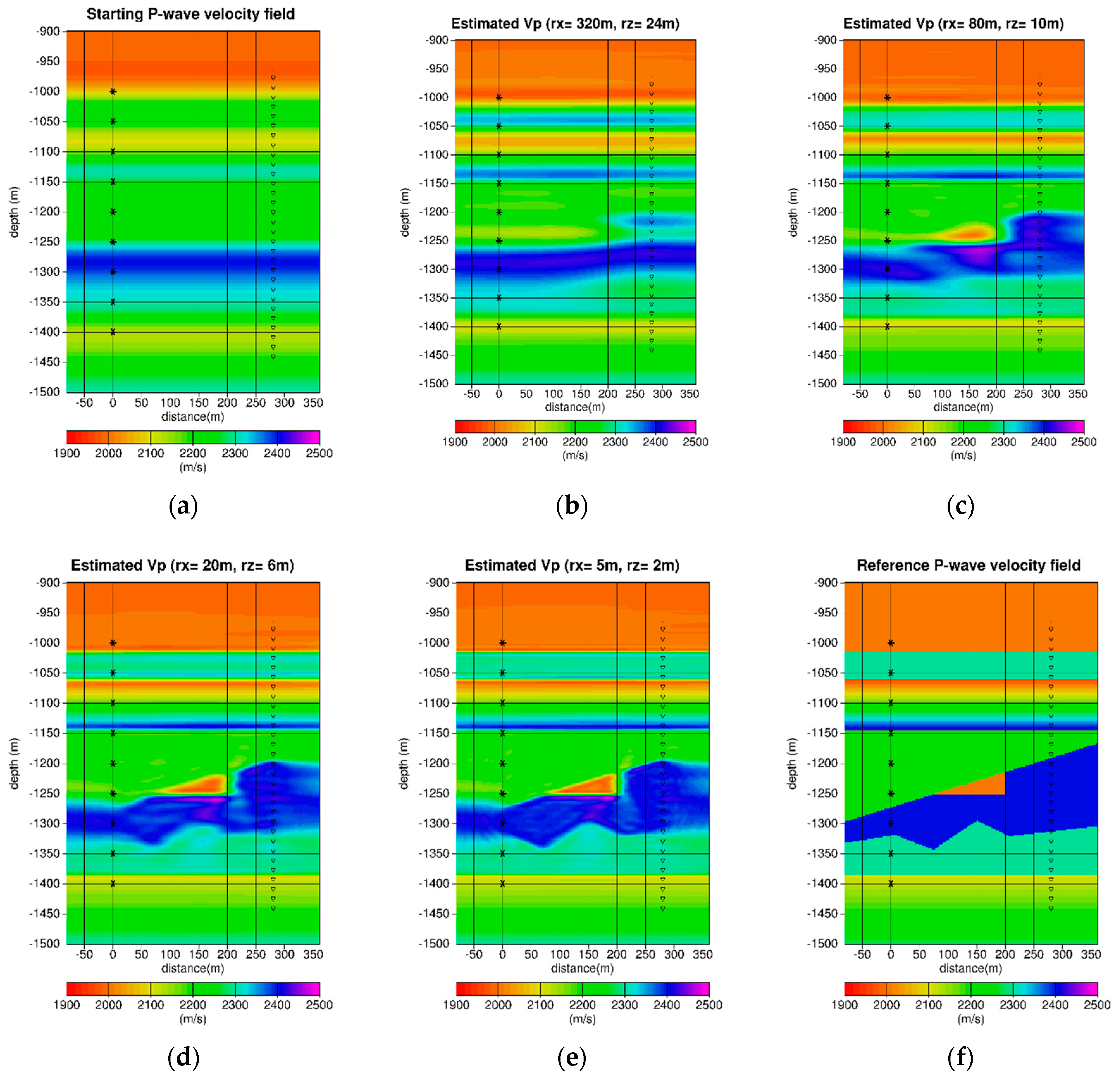
The results of the multiscale inversion process for the P-wave velocity field are displayed in Figure 6. The P-wave velocity starting model is obtained by a low-frequency full waveform inversion. It is also used as the starting model for the unconstrained inversion; such starting models can also be obtained from traveltime inversion, especially for crosswell data. The estimated P-velocity field is obtained from the first inversion scale, i.e., using correlation ranges of 320 m and 24 m in the 2D region, respectively, for the horizontal and vertical correlations. One can notice that the 2D structure cannot be resolved, as the horizontal correlation range is larger than the size of the triangular object. The 1D structures are partially retrieved. For the inversion scale (c), the estimated P-velocity field is, obtained from the inversion scale (b), i.e., using correlation ranges of 80 m and 10 m in the 2D region, respectively, for the horizontal and vertical correlations. One can notice that the 2D structure start to be resolved as both correlation ranges are smaller than the size of the triangle. The 1D structures are well estimated, with some vertical smoothening due to the vertical correlation range of 10 m. For the inversion scale (d), the estimated P-velocity field is obtained from the third inversion scale, i.e., using correlation ranges of 20 m and 6 m in the 2D region, respectively, for the horizontal and vertical correlations. One can notice that the 2D structure is getting better spatial resolution, for both the triangle and the lower zigzag interface. The 1D structures are well resolved. For the inversion scale (e), the estimated P-velocity field is obtained from the fourth and last inversion scale, i.e., using correlation ranges of 5 m and 2 m in the 2D region, respectively, for the horizontal and vertical correlations. One can notice that the delineation of the 2D structure is close to the reference model. As expected, the estimated field outside the zone between the two wells is not reliable.
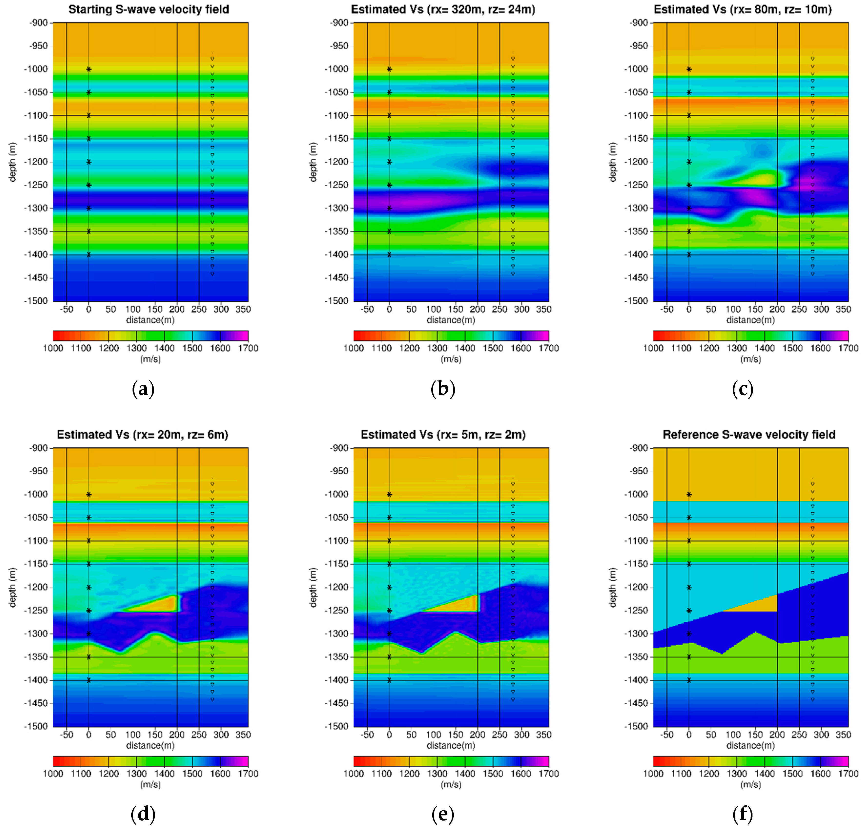
The results of the multiscale inversion process for the S-wave velocity field are displayed in Figure 7. The results are similar to the P-wave velocity field (Figure 6). The main difference is clear at the fourth scale (e): the spatial resolution is almost perfect for the S-wave due to smaller wavelength content associated to this mode. However, the inversion process provides an overestimation of velocity contrast near the interfaces and some small oscillations in the estimated field clearly visible for the light blue domain above the central triangle. It means that the number of degrees of freedom is too high regarding the amount of information provided by the data.
The misfit function for the successive multiscale inversion continuously decreases from one inversion scale to another (see Table 3).
The number of degrees of freedom per point are provided in Table 4 for the different inversion scales. These numbers of freedoms are calculated from Equation (14). The ratio of the number of degrees with respect to the number of model parameters (i.e., grid points), in other words the number of degrees of freedom per point, is provided. It is increasing slower for the quasi 1D region than for the 2D region because only the vertical correlation range is decreasing, while both horizontal and vertical ranges are decreasing in the 2D region. These ratios are pointing out that the degrees of freedom are significantly lower in the early scales of the multiscale inversion, allowing better constraint of the problem and improving the stability by defining an overdetermined system. During the last scale stages, the constraints are relaxed, allowing one to obtain a better resolution while avoiding artifacts in the estimated fields. Even for the last scale, the ratio indicates about 5 times less free parameters than in the unconstrained inversion.
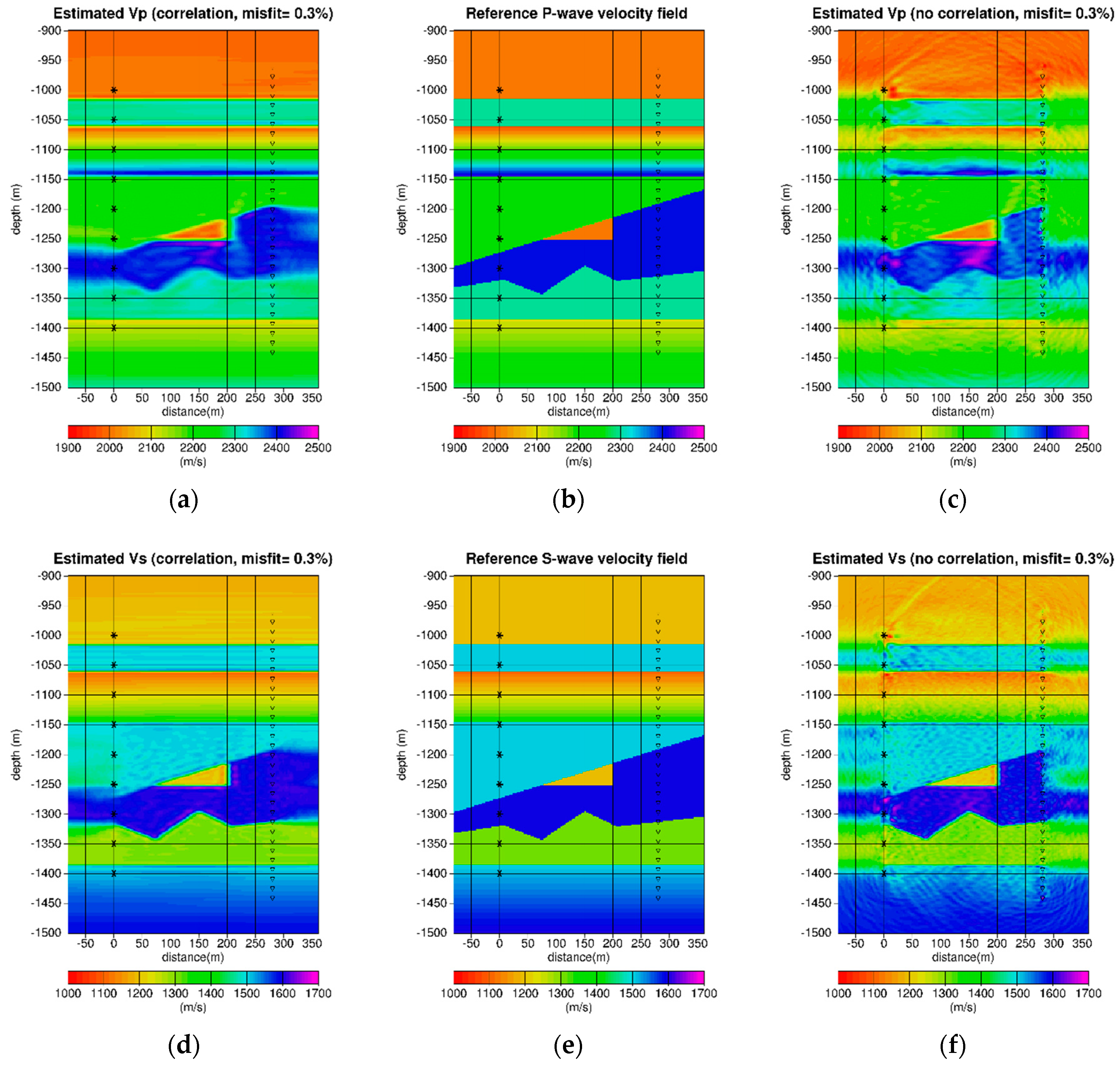
For comparison purposes with the results of the constrained inversion, we performed an unconstrained inversion. In the Figure 8, we display the results of the multiscale constrained inversion with respect to the unconstrained inversion for the same misfit of 0.3%. We can notice that the unconstrained inversion results are noisier than the constrained inversion. The main artifacts can be found near the sources (classical problem in borehole seismic full waveform inversion), below the triangle structure, above the source or receiver zones (migration smile type artifacts), and in the constant gradient 1D layers. These artifacts in the estimated fields are the consequence of the instability of the least-squares inversion problem when the problem is not correctly determined for all parameters, in other words, when it is partially underdetermined. The number of degrees of freedom is too large regarding the information provided by the data. Reducing the number of degrees of freedom of the problem taking into account prior geological information (i.e., constraining the fields using spatial statistic where we have more prior information) allows one to overcome this problem, reducing drastically the number and the magnitude of the artifacts.

5. Conclusions

In this paper, we have illustrated how to introduce, in the inverse problem, constraints consistent with the least squares formalism (through covariance matrices) on both the data and the model space.
Constraining the seismic inverse problem in the data space is not straightforward but when possible, it is a very powerful tool. In the case of a multicomponent borehole seismic data, using the polarization in the inversion process allowed better recovery of the sharpness of the interfaces at the level of the receivers.
Constraining the seismic inverse problem in the model space can be achieved by defining a priori model parameters and evaluating the model uncertainties associated with this model. Horizontal and vertical spatial correlation using Laplace distribution can be used to fill the model space covariance matrix in order to introduce an a priori information favoring the tabular region versus more complex regions, by varying accordingly the ranges of these correlations. The inversion favors solutions are consistent with our a priori, whenever it does not contradict the information contained in the data. Moreover, by adopting a multiscale type of inversion by relaxing the correlation ranges, it regularizes the inverse problem.
The incorporation of all our a priori knowledge of the parameters and all statistical studies on the data, allows not only the algorithmic stabilization of the inversion process, but also the reduction of the solution set for an underdetermined problem, with the purpose being not necessarily to converge quickly towards a good model (in term of residuals), but to prospect regions of the model space populated by models that are sensible, a priori, and also yielding the lowest possible misfit.

Author Contributions

Conceptualization, M.C. and C.B.; methodology, M.C. and C.B.; validation, M.C. and C.B.; formal analysis; writing—original draft preparation, M.C. and C.B.; writing—review and editing, M.C. and C.B.

Funding

This research received no external funding.

Conflicts of Interest

The authors declare no conflict of interest.

Appendix A

In this appendix, we will explicitly state the relation between the correlation matrix and the degrees of freedom.

Appendix A.1. Generalities

Let us consider a 1D Gaussian random field X defined in section Quantification of number of degrees of freedom and characterized by its p.d.f. given by Equation (7).
If the covariance matrix C is diagonal (i.e., no correlation between the random variables X i ), Equation (7) can be rewritten:
f ( x ) = 1 ( 2 π ) n / 2 i σ i exp ( 1 2 i ( x i m i σ i ) 2 ) = i 1 2 π σ i exp ( 1 2 i ( x i m i σ i ) 2 ) = i f i ( x i ) ,
where σ i is the standard deviation of the Gaussian random variable X i for the i t h point, and f i ( x i )   the p.d.f. associated with this variable X i . For a Gaussian field, when correlation coefficients are null, the variables X i are independent and as a consequence, the p.d.f. of the field is the product of the marginal p.d.f. of the variables, the   f i .
Assuming for simplicity that the m i and the σ i are constant, the field is made of n independent variables, identically distributed. Then, considering we have in this case n free parameters, we will study the effect of the non-independence of variables on the number of the free parameters, incorporating correlation between variables through a non-diagonal covariance matrix.

Appendix A.2. Sequential Simulation

Whatever the discrete random field, the knowledge of the joint p.d.f. (like f defined in Equation (7) for the Gaussian random field X ) allows simulation of a realization of the field sequentially, using the marginal-conditional decomposition (correct whatever the order of the indexes):
f ( x 1 , x 2 , , x n ) = g 1 ( x 1 ) · g 2 ( x 2 | x 1 ) · g 3 ( x 3 | x 1 , x 2 ) · · + g n ( x n | x 1 , x 2 , x n 1 ) ,
where g i is the marginal-conditional p.d.f. of the random variable X i , independently of the random variables X j for   j > i   and conditionally to the random variables   X k for k < i . More precisely, g i is defined by the relation:
g i ( x i | x 1 , x 2 , , x i 1 ) =   d x i + 1   d x i + 2   d x n   f ( x 1 , x 2 , , x n )   d x i   d x i + 1   d x n   f ( x 1 , x 2 , , x n ) .
Using Equation (A2), it is possible to simulate a realization of the field sequentially. First, we use g 1 ( x 1 )   to generate a realization of the random variable   X 1 , independently of all other variables. Once x 1 = x 1 0 is determined, we use g 2 ( x 2 | x 1 0 ) to generate a realization x 2 0 of the random variable   X 2 , dependent to the value x 1 0 , but independent of the other random variables   X 3 to   X n . We repeat this procedure using g 3 , then g 4 , and so on, until the last value x n 0 is determined, thereby obtaining a realization x 0 of the random field X .
We can link the degree of freedom of the variable   X i , when the values x i to x i 1   are known, to the standard deviation σ i c of the Gaussian defined by the p.d.f. g i ( x i | x 1 , x 2 , , x i 1 ) . To account for the correlation between the variables   X i , independently of the values of the standard deviations   σ i of the marginal p.d.f. f i ( x i ) , we can then define the degrees of freedom of the variable   X i (when x 1 to x i 1 are known) as the following ratio:
d = σ i c   σ i   ,
which equals one when   X i is not correlated to the variables ( X 1 ,   X 2 , , X i 1 ) and zero when the correlation is perfect.

Appendix A.3. The L U Simulation Technique

In order to simplify the calculation of the degrees of freedom, we introduce here the L U decomposition technique for Gaussian field simulation, as this method can be interpreted in term of sequential simulation using Equation (7).
A way to simulate a Gaussian discrete random field X defined by the p.d.f. in Equation (A2) ( n points with expectation m and covariance matrix   C ) is the use of the L U decomposition of the covariance matrix   C :
C = L U = L L T   ,
where L denotes the left lower triangle matrix and U the upper right one.
Considering a random field E constituted by n random variables, independently and identically distributed following a Gaussian law with zero mean and unit standard deviation; the field   m + L E is then equivalent to   X . Therefore, to simulate a realization x of the random field   X , we can use a realization e of the field E and write:
x = m + L e     .

Appendix A.4. Interpretation of the L U Decomposition of the Covariance Matrix

Let l i j be the elements of the matrix   L . The relation given by Equation (A6) can be interpreted in term of sequential simulation: the first line gives x 1 = m 1 + l 11 e 1 , meaning that we simulate the realization of X 1 independently of the other variables, as if we used the 1 D marginal p.d.f. g 1 ( x 1 )   defined in Equation (A2):
g 1 ( x 1 ) = 1 2 π σ 1 exp ( 1 2 ( x 1 m 1 σ 1 ) 2 ) = f 1 ( x 1 ) .
Once the value of x 1 is fixed, the second line of the Equation (15) means that the second random variable x 2 can be written:
X 2 = m 2 + l 21 e 1 + l 22 E 2 = m 2 + l 21 ( x 1 m 1 l 11 ) + l 22 E 2 ,
Meaning that we simulate the realization of X 2 independently of X 3 , , X n but dependent of the value X 1 = x 1 , as if we used the conditional marginal p.d.f. g 2 ( x 2 | x 1 ) (see Equation (A2)). A given line i of the Equation (A6) means we can simulate a random variable X i conditionally to the determined values of the preceding variables x 1 to x i 1 , as if we used the proper marginal-conditional p.d.f. g i ( x i | x 1 , x 2 , , x i 1 ) (see Equation (A2)).
Let us come back to the estimation of the degrees of freedom. The standard deviations σ i c are given here by the i t h diagonal element l i i of the matrix L . This standard deviation is lesser than the standard deviation of the variable X i , independently of the other variables (i.e., the standard deviation σ i of the Gaussian defined by the marginal p.d.f. f i ( x i ) ). When correlation between Xi and the variables X 1 to X i 1 is strong, the ratio l i i σ i is weak. When X i is independent of the variables X 1 to X i 1 , the ratio equals 1, meaning the freedom of the variable is total. We can say that when variables are independent (no correlation), the number of the free parameters is n = i 1 1 and when correlation exists, it is reduced to:
N = i l i i σ i .

Appendix A.5. The L U Decomposition of the Correlation Matrix R

The covariance matrix can be written with the following form:
C = S R S ,
where R is the correlation matrix and S the diagonal matrix of the standard deviations;
S = ( σ 1 0 0 0 σ 2 0 0 0 σ n ) .
The L U decomposition of R gives: R = M M T , with L = S M . Therefore, the field X can be written (see Equation (20)):   X = m + L E = m + S M E .
The number of free parameters is then:
N = i l i i σ i = t r a c e ( M ) .

Appendix B

Let us consider a pair of random variables ( X , Y ) characterized by the following p.d.f.:
f ( x , y ) = 1 2 π det ( C ) exp ( 1 2 ( x m x y m y ) T C 1 ( x m x y m y ) ) ,
where C is the covariance matrix, we have:
C = ( σ x 2 ρ σ x σ y ρ σ x σ y σ y 2 ) ,   d e t ( C ) = σ x 2 σ y 2 ( 1 ρ 2 ) ,   C 1 = 1 1 ρ 2 ( 1 σ x 2 ρ σ x σ y ρ σ x σ y 1 σ y 2 ) ,
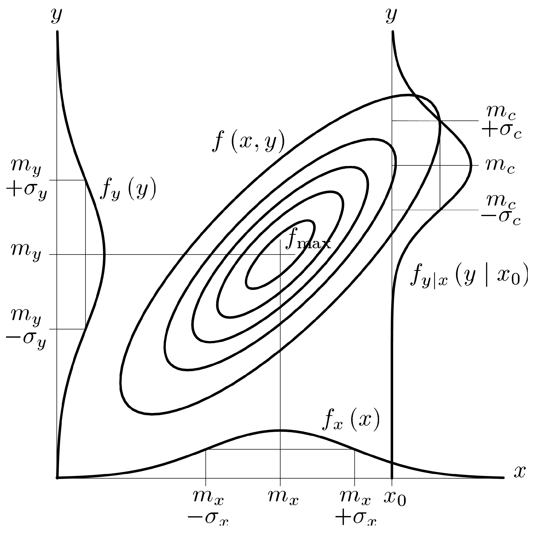
where ρ is the correlation between the random variables X and Y . An example is given in Figure A1, with the following values: m x = m y = 0 , σ x = σ y = 1 , ρ = 4 / 5 .
Equation (16) of the decomposition of the p.d.f. is written:
f ( x , y ) = f 1 ( x ) f 2 ( y | x ) ,
where
f x ( x ) = 1 2 π σ x exp ( 1 2 ( x m x σ x ) 2 ) f y | x ( y | x ) = 1 2 π σ y 1 ρ 2 exp ( 1 2 ( y m y ρ σ y ( x m x σ x ) σ y 1 ρ 2 ) 2 ) .
We can note that the characteristics of these p.d.f. are given by the elements of the left triangle matrix of the covariance L U decomposition:
L = ( σ x 0 ρ σ y σ y 1 ρ 2 ) .
Indeed, the first line corresponds to the standard deviation of the p.d.f. f x ( x ) . The conditional p.d.f. f y | x ( y | x ) is plotted on Figure A1. It is characterized by its mean m c = m y +   ρ σ y ( x m x σ x ) and its standard deviation σ c = σ y 1 ρ 2 . In the second row, the first element corresponds to the scale factor of the correction of the mean of the conditional p.d.f. f y | x and the second element to the standard deviation of the conditional p.d.f. In summary, the diagonal elements are the standard deviations of the random variables X and   Y | X . The effect of the correlation   ρ is to reduce, by the factor   1 ρ 2 , the degree of freedom of the second variable Y when X is known, as we see in Figure A1. We then note that the total degree of freedom of this pair is (taking as a reference the uncorrelated pair characterized by the diagonal covariance matrix,   ρ = 0 ):
d = σ x σ x + σ y 1 ρ 2 σ y = 1 + 1 ρ 2 .
We can note that   d = 1 when the correlation is perfect ( ρ = ± 1 ) and d = 2 when the correlation is inexistent ( ρ = 0 ).
Figure A1. The joint probability density f ( x , y ) of the couple of random variables ( X , Y ) is plotted using contour levels (at level 0.9 · f m a x , 0.7 · f m a x , 0.5 · f m a x , 0.3 · f m a x and 0.1 · f m a x ), the marginal probability densities for the variables themselves ( f x ( x ) for X and f y ( y ) for Y ) are plotted on the x and the y axes. The value x 0 = 1.5 has been fixed and the conditional probability density f c ( y ) = f y | x ( y | x 0 ) is plotted, the mean m x = m y = 0 and m c has been reported as the standard deviation σ x = σ y = 1 and σ c , the correlation ρ = 0.8 appears only in the ellipticity of the ellipses for the joint p.d.f. f . As Equation (A17) shows, the number of free parameters of the couple ( X , Y ) is 1 + σ c σ y = 1 + 1 ρ 2 = 1.6 .
Geosciences 09 00045 g0a1

References

  1. Virieux, J.; Operto, S. An overview of full waveform inversion in exploration geophysics. Geophysics 2009, 74, WCC1–WCC26. [Google Scholar] [CrossRef]
  2. Menke, W. Geophysical Data Analysis: Discrete Inverse Theory; Academic Press, Inc.: Orlando, FL, USA, 1984. [Google Scholar]
  3. Tarantola, A. Inverse Problem Theory: Methods for Data Fitting and Model Parameter Estimation: Discrete Inverse Theory; Elsevier Science Publ. Co., Inc.: New York, NY, USA, 1987. [Google Scholar]
  4. Tikhonov, A.; Arsenin, V. Solution of Ill-Posed Problems; Winston: Washington, DC, USA, 1977. [Google Scholar]
  5. Operto, S.; Virieux, J.; Dessa, X.; Pascal, G. Crustal imaging from multifold ocean bottom seismometers data by frequency-domain full-waveform tomography: Application to the eastern Nankai trough. J. Geophys. Res. 2006, 111, B09306. [Google Scholar] [CrossRef]
  6. Guitton, A.; Ayeni, G.; Gonzales, G. A preconditioning scheme for full waveform inversion. In SEG Technical Program Expanded Abstracts 2010; Society of Exploration Geophysicists: Tulsa, OK, USA, 2010; pp. 1008–1012. [Google Scholar] [CrossRef]
  7. Guitton, A. A blocky regularization scheme for full waveform inversion. In SEG Technical Program Expanded Abstracts 2011; Society of Exploration Geophysicists: Tulsa, OK, USA, 2011; pp. 2418–2422. [Google Scholar] [CrossRef]
  8. Abubakar, A.; Hu, W.; Habashy, T.M.; van den Berg, P.M. Application of the finite-difference contrast-source inversion algorithm to seismic full-waveform data. Geophysics 2009, 74, WCC47–WCC58. [Google Scholar] [CrossRef] [Green Version]
  9. Herrmann, F.J.; Erlangga, Y.A.; Lin, T.T.Y. Compressive simultaneous full-waveform simulation. Geophysics 2009, 74, A35–A40. [Google Scholar] [CrossRef]
  10. Loris, I.; Douma, H.; Nolet, G.; Daubechies, I.; Regone, C. Nonlinear regularization techniques for seismic tomography. J. Comput. Phys. 2010, 229, 890–905. [Google Scholar] [CrossRef] [Green Version]
  11. Asnaashari, A.; Brossier, R.; Garambois, S.; Audebert, F.; Thore, P.; Virieux, J. Regularized seismic Full-waveform inversion with prior model information. Geophysics 2013, 78, R25–R36. [Google Scholar] [CrossRef]
  12. Asnaashari, A.; Brossier, R.; Garambois, S.; Audebert, F.; Thore, P.; Virieux, J. Time-lapse seismic imaging using regularized full-waveform inversion with a prior model: Which strategy? Geophys. Prospect. 2015, 63, 78–98. [Google Scholar] [CrossRef]
  13. Polak, E.; Ribière, G. Note sur la convergence de directions conjuguée. Rev. Fr. Inform. Rech. Oper. 3e Année 1969, 16, 35–43. [Google Scholar]
  14. Crase, E. Robust Elastic Nonlinear Inversion of Seismic Waveform Data. Ph.D. Thesis, University of Houston, Houston, TX, USA, 1989. [Google Scholar]
  15. Jurkevics, A. Polarization analysis of the three component array data. Bull. Seismol. Soc. Am. 1988, 78, 1725–1743. [Google Scholar]
  16. Virieux, J. P-SV wave propagation in heterogeneous media: Velocity-stress finite-difference method. Geophysics 1986, 51, 889–901. [Google Scholar] [CrossRef]
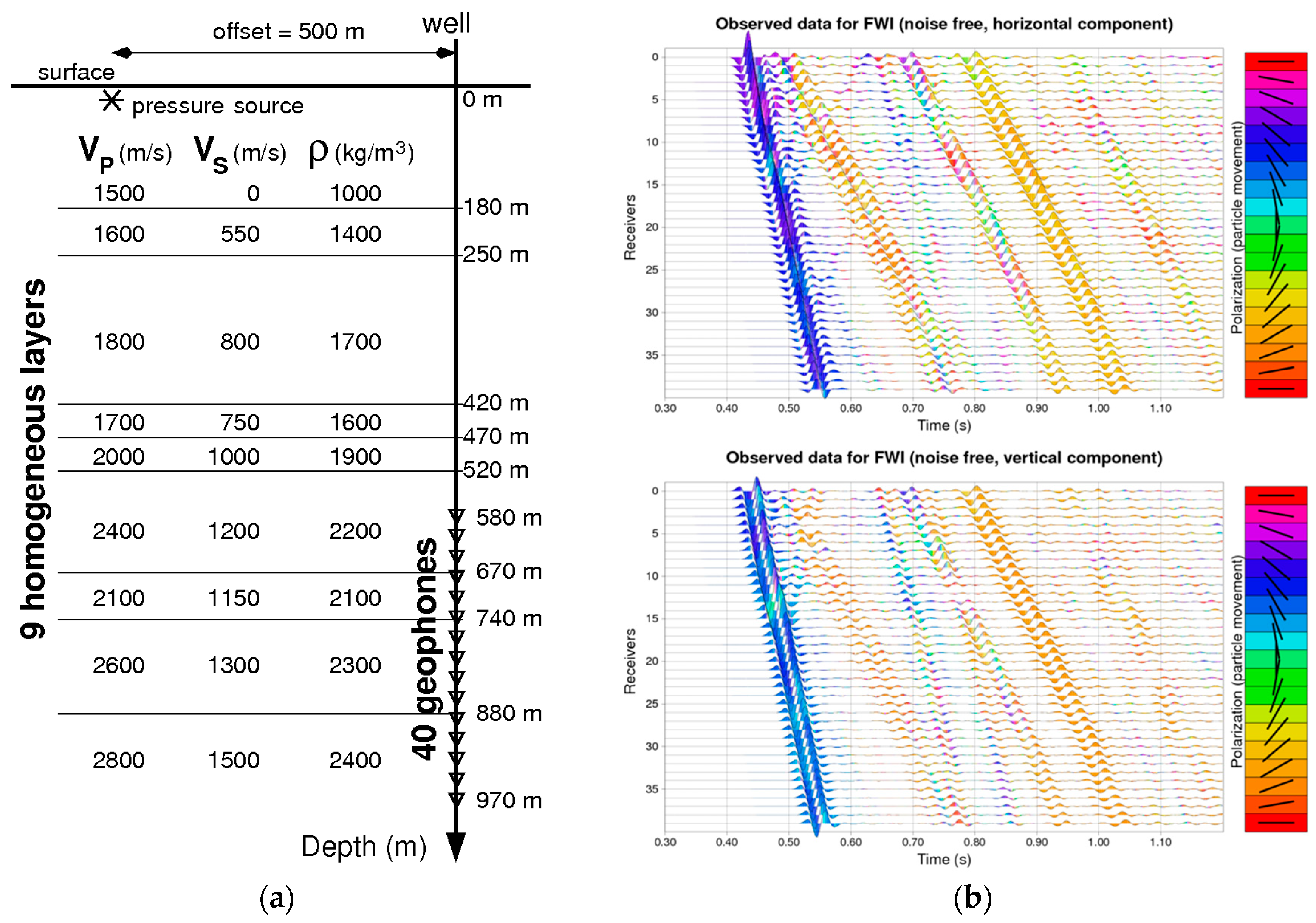
Figure 1. Offset Vertical Seismic Profile (OVSP) numerical experiment: (a) Synthetic experiment configuration where the asterisk near the surface denotes the source position for the unique shot point, whereas the triangles in the well denote the location of the 40 two-component geophones. The “true” model is composed of nine homogeneous layers, the first one being the water layer. This true model is used both to model the observed data and as a reference to check inversion results; (b) the horizontal (top) and vertical (bottom) components of the ground velocity field recorded at geophones—the fields are obtained by modeling the wave equation in the true model (finite difference approximation). The color represents the local polarization estimated using a 2-period time window.
Geosciences 09 00045 g001
Figure 2. Two inversion experiments with and without polarization constraints. (a) Without polarization constraints for P-wave velocity estimated model. (b) With polarization constraint for P-wave velocity estimated model. (c) Without polarization constraints for S-wave velocity estimated model. (d) With polarization constraints for S-wave velocity estimated model. In all plots: red thick solid line denotes the true model we want to retrieve by inverting the observed data; gray solid line denotes the starting model in the inversion process; blue, green, and black solid lines denote estimated models from inversion, respectively, at iterations 10th, 30th, and 80th. The vertical thick black solid line indicates the level of the receiver antenna. The constrained inversion contributes to the recovery of the sharp interfaces, especially at the level of the receiver antenna.
Geosciences 09 00045 g002
Figure 3. Degree of freedom per point (for a regular grid) as a function of the range (expressed in multiples of the grid step) of the correlation for a Laplace correlation function.
Geosciences 09 00045 g003
Figure 4. The reference velocity models: (a) Reference P-wave velocity field; (b) reference S-wave velocity field. The source borehole is located at 0 m distance and the nine asterisks (*) denote the source locations for the nine shots. The receiver borehole is located at 280 m offset and the small triangles denote the locations of the receivers. On can notice that the structures of these reference velocity fields are the same for P- and S-wave. It is composed of 1D regions (invariance along the horizontal axis) in the upper part of the model and at the bottom with homogeneous layers and other layers with a velocity increasing linearly with depth (vertical constant gradient). The middle part of the model exhibits complex 2D structures.
Geosciences 09 00045 g004
Figure 5. The 5th shot, at 1200 m deep, of the observed data obtained by full-wave modeling from the reference models: (a) The horizontal component; (b) the vertical component. The source function is a first derivative of a Gaussian with a central frequency of 100 Hz and it acts as a stress source with the following radiation coefficients σ x x = 1   , σ z z = 0.5 , σ x z = 0 . These data are used as observed data in the multiscale inversion process.
Geosciences 09 00045 g005
Figure 6. The results of the multiscale inversion process for the P-wave velocity field. Stars denote the source location while the small triangles denote the receiver location: (a) The P-wave velocity starting model; (b) the estimated P-velocity field obtained from the first inversion scale using correlation ranges of r x = 320   m   and r z = 24   m in the 2D region; (c) the estimated P-velocity field obtained from the second inversion scale using correlation ranges of r x = 80   m   and r z = 10   m in the 2D region; (d) the estimated P-velocity field obtained from the third inversion scale using correlation ranges of r x = 20   m   and r z = 6   m in the 2D region; (e) the estimated P-velocity field obtained from the fourth and last inversion scale using correlation ranges of r x = 5   m   and r z = 2   m in the 2D region; (f) the reference P-wave velocity model. The results for the first scale of the inversion do not allow recovery of the 2D structures, as the correlation ranges are greater than the size of the objects. The 2D structures start to appear from the second scale, improving from the third scale, and are well recovered for the last scale.
Geosciences 09 00045 g006
Figure 7. The results of the multiscale inversion process for the S-wave velocity field. Stars denote the source location while the small triangles denote the receiver location: (a) The S-wave velocity starting model; (b) the estimated S-velocity field obtained from the first inversion scale using correlation ranges of r x = 320   m and r z = 24   m in the 2D region; (c) the estimated S-velocity field obtained from the second inversion scale using correlation ranges of r x = 80   m   and r z = 10   m in the 2D region; (d) the estimated S-velocity field obtained from the third inversion scale using correlation ranges of r x = 20   m   and r z = 6   m in the 2D region; (e) the estimated S-velocity field obtained from the fourth and last inversion scale using correlation ranges of r x = 5   m   and r z = 2   m in the 2D region; (f) the reference S-wave velocity model. The S-wave estimated field exhibits a better spatial resolution than the P-wave (see Figure 6) due to the smaller wavelength content associated with this mode. Small artifacts can be observed around the 2D triangle structure, pointing out the fact that the problem is less constrained in this part of the model.
Geosciences 09 00045 g007
Figure 8. Comparison between results from the constrained inversion using the multiscale inversion process results of the multiscale inversion process and results from the unconstrained inversion: (a) The estimated P-wave velocity field for the multiscale inversion for a misfit of 0.3%; (b) the reference P-wave velocity field; (c) the estimated P-wave velocity field for the unconstrained inversion for a misfit of 0.3%; (d) the estimated S-wave velocity field for the multiscale inversion for a misfit of 0.3%; (e) the reference S-wave velocity field; (f) the estimated S-wave velocity field for the unconstrained inversion for a misfit of 0.3%. Both P- and S-wave estimated fields show that the multiscale inversion results are smoother than the unconstrainted inversion results, with well artifact and better reliability. The main artifacts are near the sources, below the triangle structure, above the source or receiver zones and below (less visible due to the color range), and in the constant gradient 1D layers. As expected, there is no additional information outside the square delimited by the wells for the case of unconstrained inversion.
Geosciences 09 00045 g008
Table 1. A priori geological region type with respect to depth.
Depth (m)Region TypeNumber of Vertical Points
800–1120Quasi 1D161
1120–1180Transition29
1180–13402D81
1340–1400Transition29
1400–1600Quasi 1D101
Table 2. Horizontal and vertical correlation ranges for the different a priori region types and inversion scales.
Region TypeCorrelation Ranges (m)Inversion Scale (b)Inversion Scale (c)Inversion Scale (d)Inversion Scale (e)
Quasi 1D ( r x ,     r z ) (1000, 24)(1000, 10)(1000, 6)(1000, 2)
2D ( r x ,   r z ) (320, 24)(80, 10)(20, 6)(5, 2)
Table 3. The misfit and iteration number for the different inversion scales.
Inversion ParametersInversion Scale (b)Inversion Scale (c)Inversion Scale (d)Inversion Scale (e)
Initial Misfit45.5%27.9%6.55%0.81%
Final Misfit27.9%6.55%0.81%0.14%
Iteration #30305050
Table 4. Number of degrees of freedom (DoF) per point for the successive multiscale inversions.
Region TypeInversion Scale (b)Inversion Scale (c)Inversion Scale (d)Inversion Scale (e)
Quasi 1D1919281234164554
Transition267468622857
2D10222922679215,725
All3208620210,83021,136
DoF/point2.8%5.5%9.6%18.8%