1. Introduction
An increase in more severe climatic changes in seasonal temperatures has contributed to unpredictable rates of water flow in rivers, most commonly flood events and increasing frequency [
1,
2,
3,
4,
5], and resulted in economic disaster [
6]. Floods are the primary natural disaster for the highest mortality rate in 2016 even though this number drops every year and the cost increases [
7]. Worldwide, flood events result in severe damages and count up to billions of dollars bringing up floods as the most significant hazard among all natural economic disasters [
8,
9]. In Schenectady, New York the flood events are due to either an increase in precipitation and storms during the summer or ice jams in the winter months. Ice jams occur when floes accumulate at the base of bridge piers, locks, and dam structures, impeding the downstream water flow causing an upstream rise in the water level [
10,
11]. Flood forecasting research has been conducted in the past at Schenectady in which flood forecasting and damage evaluation has been surveyed [
12,
13,
14,
15,
16,
17]. In this study, we use hydrogeological and climatic data to predict the water discharge time series in Mohawk River at Schenectady, New York. For the analysis, we combine the time series decomposition and the time series regression model (TSR) model to predict the water discharge time series. The reason that the TSR model has been chosen was due to the advantage of physical interpretation for the variables which may contribute to a flood event. Other models may provide higher or lower forecasting power, but they may lack for the physical interpretation of the variables included in the model [
14,
18,
19,
20]. The climatic and hydrogeological data consists of a sufficient amount of daily records and frequent extreme events among natural seasonal phenomena. To reveal the periodical phenomena based on lags between the predictor variables, we use the time series decomposition applied to the climatic and hydrogeological variables. We also intend to explore the implications and the effect of lags between the water discharge time series and the independent variables applied to each time series component.
To isolate the different cycles in the time series and eliminate the interferences between the cycles, we decompose the time series of the water discharge and the hydrogeological and climatic variables into the long, seasonal and short-term component [
14]. Several studies have shown that the decomposition of the variables into different components may isolate the noise from the data and separate the different signals in the time series [
14,
21,
22]. The multiple linear regression model (MLR) uses only the current values for the explanation of the water discharge. In this study, we use the TSR instead of the MLR model to include the current and past values of the independent variables for the explanation of the water discharge time series.
Time series regression models in flood forecasting have been numerously utilized [
23,
24,
25], and it is pertinent to forecasting floods because linear regression requires an inference about the correlation between the dependent and independent variables. Although the multiple linear regression model is a very well known model for flood forecasting, it is constrained by integrating current values. Thus for integrating the current and past values, we use the TSR model.
The TSR model is a statistical model that includes current and past observations of the predictors’ variables and can be used for forecasting an event applied in several fields [
26,
27,
28,
29]. The hydrogeological and climatic data have shown in a previous analysis [
14] seasonality and periodicities ranging from a couple of weeks to an annual cycle. The application on the data of a time series model (i.e., ARIMA model) or a multiple regression model without the decomposition of the time series may lead to inaccurate results and lack of physical interpretation due to the mixed cycles on the data [
30,
31].
Previous studies have shown that using the linear regression model with the lag on the variables, the model accuracy has been increased [
32]. A lag relationship is a time-delayed correlation where one or more independent variables are time correlated with a delay in the dependent variable.
When a variable fluctuates earlier than another dependent variable the correlation may be obscured. The cause and effect are displaced in time, and lag operators may bridge this gap and reveal a significant correlation. However, in multivariate linear regression, there are interferences and collinearity between the independent variables that may provide spurious correlations. In this paper, we provide an example of how decomposition solves this issue by separating different cycles of variables at different time scale components and permits the lag operation to reveal significant correlations and subsequent physical interpretation. The decomposition of the hydrogeological and climatic time series and the incorporation of the lags in the independent variables the forecasting accuracy of the model has been increased compared to the raw data. This model can be used for warning the residents of a possible flood event and can be applied in other locations, as well.
3. Data
The information obtained from the climatic and hydrogeological stations and referred to the equations have been abbreviated to average wind speed (WS; mph miles to tenths), Fastest 5 s Wind Speed (F5SWS; mph miles to tenths), precipitation (PR; inches to hundredths), snow (S; inches to the tenths), snow depth (SD; inches), maximum temperature (T; °C), humidity (H; % of water the air can hold), atmospheric air pressure (P; inches of mercury, to hundredths), tides (TD; meters), water discharge (WD; cubic meters per second), groundwater depth upstream (GWU; meters), groundwater depth downstream (GWD; meters) and the difference between the measured distance from the surface to the water level at the upstream groundwater station subtracted from the associated distance at the downstream groundwater station (GWDIF; meters).
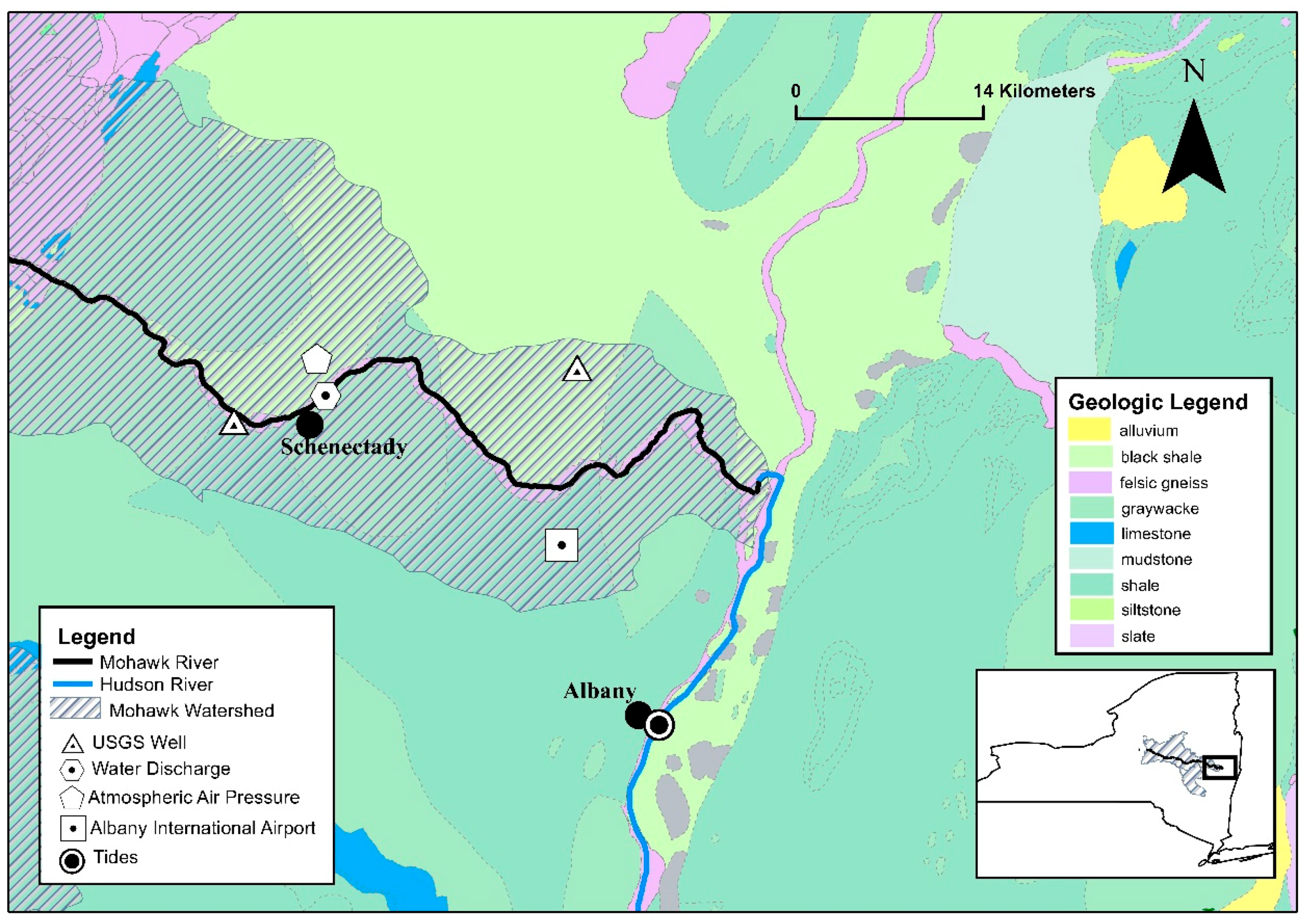
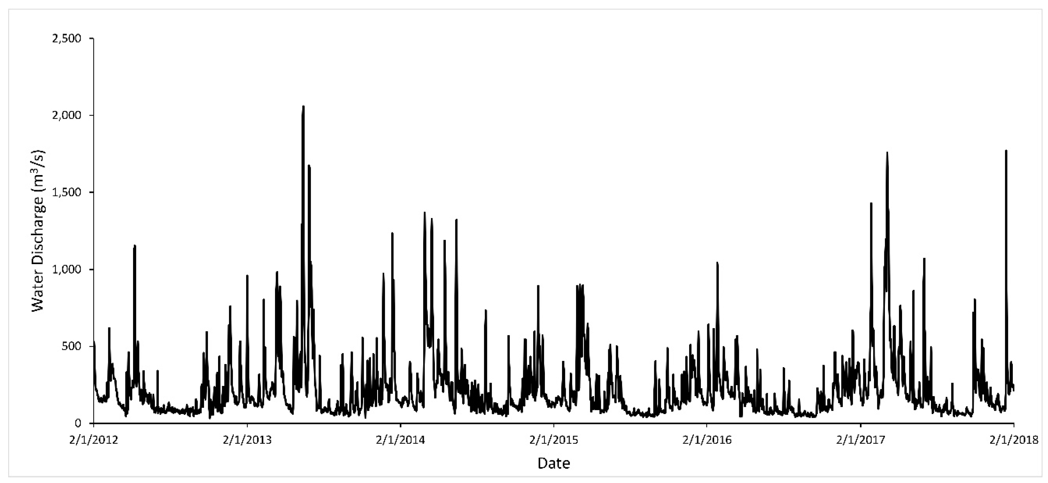
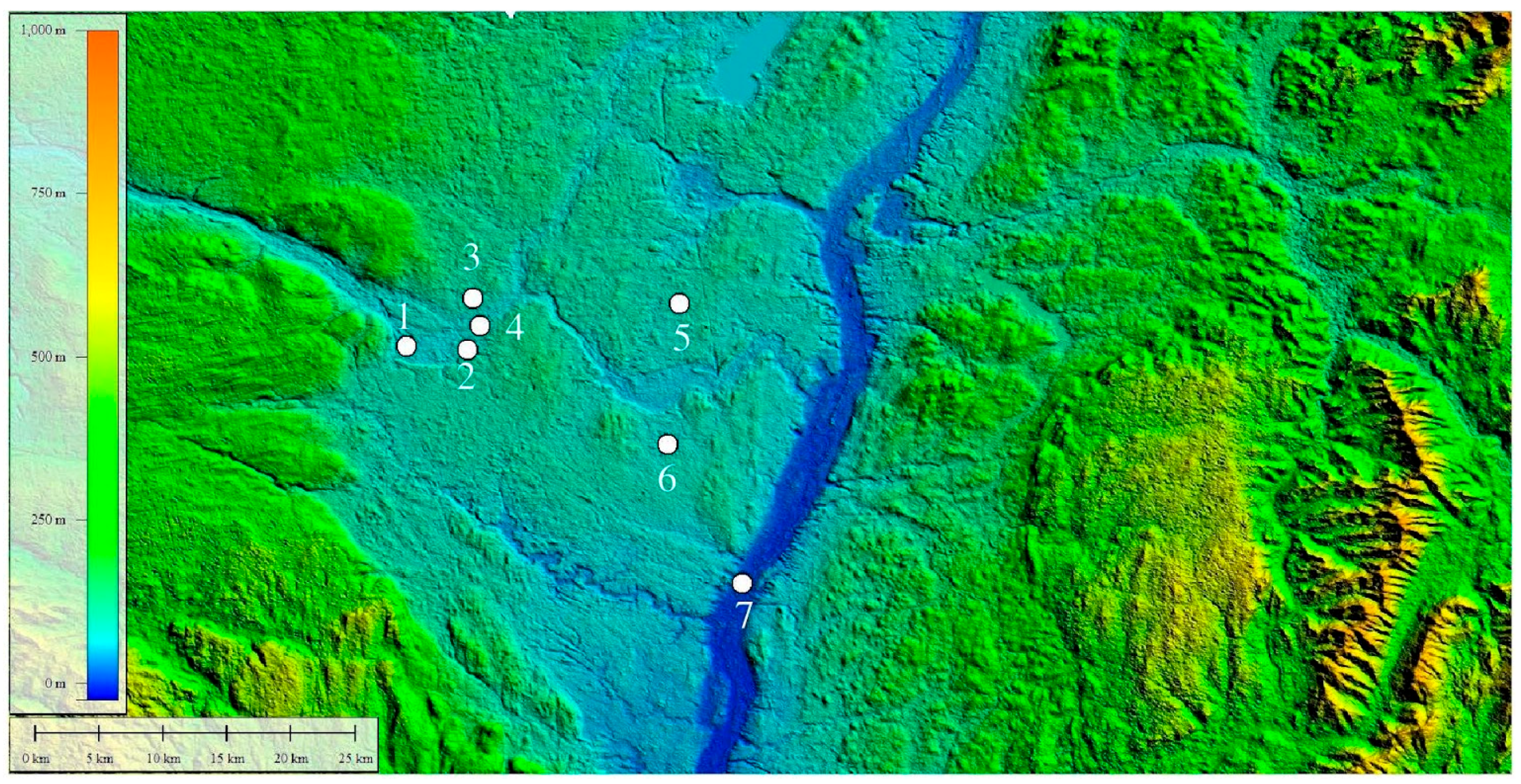
Atmospheric and hydrological data (water discharge and groundwater) measured from 1 February 2012 to 1 February 2018, were obtained from stations located near Schenectady, NY (
Figure 1): Water discharge Station Id 01354500 01354500 (
https://waterdata.usgs.gov/ny/nwis/uv/?site_no=01354500&PARAmeter_cd=00065,00060) (
Figure 2; lat-42°49′49.9′′ N, lon-73°55′50.7′′ W), groundwater level from the downstream area of the station USGS Well 425048073472501 which is referred to this paper as GWD (
https://waterdata.usgs.gov/ny/nwis/uv/?site_no=424859073585501&PARAmeter_cd=72019,62610,62611); (lat-42°50′47.0′′ N, lon-73°47′26.9′′ W), groundwater level from the upstream area of the station USGS Well 424859073585501 which is referred to this paper as GWU (
https://www.ncdc.noaa.gov/cdo-web/datasets/NORMAL_DLY/stations/GHCND:USW00014735/detail) (lat-42°48′59′′ N, lon-73°58′55′′ W), Albany Airport Weather Station GHCND:USW00014735 (
https://www.ncdc.noaa.gov/cdo-web/datasets/LCD/stations/WBAN:04741/detail) (lat-42.74722° N, lon-73.79912° W), Atmospheric air pressure Data Station WBAN 04741 (
https://tidesandcurrents.noaa.gov/noaatidepredictions.html?id=8518995) (lat-42°51′00.0′′ N, lon-73°56′08.7′′ W) and Tide Data- Station ID 8518995 (lat-42°39.0′ N, lon-73°44.8′ W).
4. Methods
A digital elevation model (DEM) was produced in Global Mapper 17.2 (Hallowell, ME, USA) with the locations of the monitoring stations of the study area. Locations of the stations were projected in a DEM to identify any physical boundaries that may obstruct the measurements for the selected monitoring stations (
Figure 3).
The data collection of the monitoring stations and preprocessing was performed in KNIME which is an open source data analytics and data mining software. The workflow system KNIME [
36] is an open source software. Knime is composed of different processing nodes that pass data to each other complemented with titles, annotations, and descriptions. Output tables are stored in memory eliminating correlations between 13,410 variables, tables and associated variables being stored in separate files as our research required. KNIME software provides another way of script-free data processing without excluding the utilization of Python in various processing nodes. Although occasionally java is required, available nodes in an extensive available catalog of processing nodes provided by the open community dramatically facilitate complex statistical processing. Notable libraries include such for statistical time series analysis and regression models [
37]. KNIME has become very useful for various data mining or statistical applications and machine learning [
38,
39,
40], and we have found it very efficient for the decomposition. The decomposition of different time scales has a prerequisite of joining multiple tables and databases; therefore, a software such as KNIME was appropriate for this application. The extracted raw data were retrieved from their original URL sources, and 15-min, hourly, and daily data were obtained for the specific location (
Figure 4). For the analysis, all the data were converted to a daily time series considering the maximum value per day.
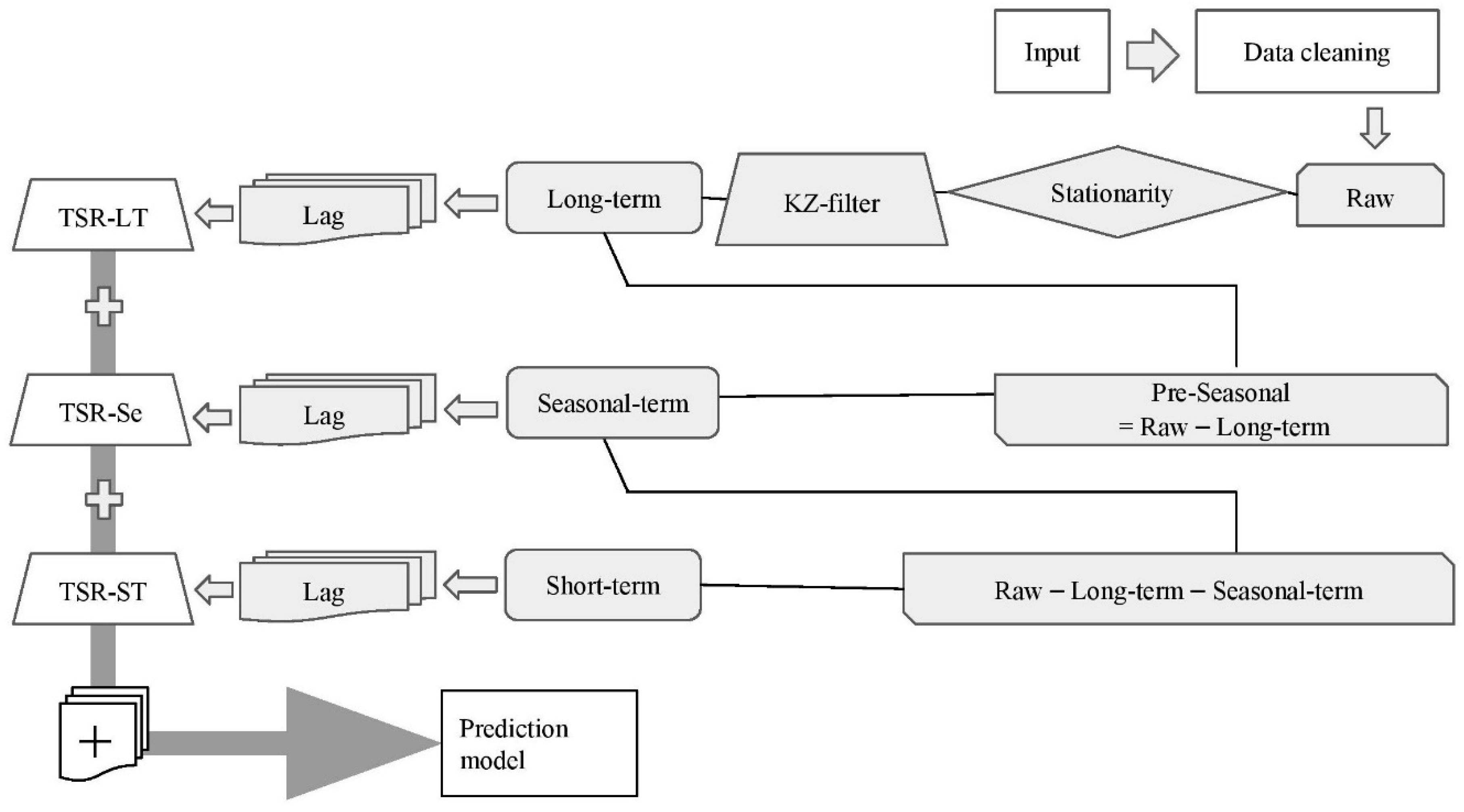
A flowchart describes the methodology for the decomposition of the time series of all the variables and the application of the time series regression model in the long-term, seasonal-term, and short-term component (
Figure 4). To stabilize the variance of the data for the series to be stationary, we use the log transform of the variable [
14]. For our study, the log transformation of the water discharge time series is named as the raw data (
Figure 4). The decomposition of the time series of a variable can be expressed by Equation (1):
where X(t) is the original time series of a variable, LT(t) is the long-term trend component, Se(t) is the seasonal-term component, and ST(t) is the short-term component. The long-term component represents the fluctuations of a time series longer than a given threshold, the seasonal component describes the year-to-year fluctuations, and the short-term component represents the short-term variations.
For the decomposition of the time series, we use the Kolmogorov-Zurbenko (KZ) filter. The KZ filter is a low pass filter, defined by p iterations of a simple moving average of m points. The moving average of the KZ was performed by the Equation (2):
where m = 2k + 1
The output of the first iteration becomes the input for the second iteration, and so on. The time series produced by p iterations of the filter described in Equation (2) and it is denoted by Equation (3):
The parameter m in Equation (3) has been determined to provide the maximum explanation of the water discharge times series by the climatic variables. The parameters of the model have been chosen as a physical based explanation for the dependent variable [
22]. For this study, the KZ
33,3 filter (length of thirty-three with three iterations) has been applied in all the variables and obtained the long-term (LT) values as depicted in the flowchart (
Figure 4).
The pre-seasonal time series (SE
PRE) can be estimated by the difference between the raw data and the long-term component using the Equation (4):
Also, the seasonal component of the time series, Se(d), can be defined by Equation (5):
In Equation (5), d represents the days of a year, y is the number of years of the observed values, and SEPRE is the pre-seasonal time series described by Equation (4). The seasonal components of the climatic and hydrogeological variables can be defined similarly.
Using Equation (1), the short-term (ST) component of each variable can be determined by Equation (6):
where X(t) is the original time series, LT(t) is the long-term component, and Se(t) is the seasonal-term component.
For the prediction of the water discharge, we use the time series regression model. The time series regression (TSR) is a statistical method for predicting a future response variable and transfer the dynamic from relevant predictors. For this study, the response variable is the water discharge time series, and the predictor variables are the climatic and hydrogeological variables. The TSR model is described by the Equation (7):
where Y(t) is a response vector which represents the water discharge time series, Z(t) is the predictor vector which represents the climatic and hydrogeological variables, b represents the linear parameter estimates, and ε(t) represents the residuals terms. The predictor vector consists of current and past observations of the climatic and hydrogeological variables that is the lagged-variables.
Two parameters were set up for computing the lag of a variable. The lag interval l is the time shifting for each variable. The lag L arranges the number of times that data shift in a column. The lag operator was performed in each variable that is sorted in time increasing order. We have assigned a lag L of 365-days to make L copies of each independent variable and shift the cells of each variable by L−1 steps down with a lag interval l equal to 1-day. Each variable-column shifted by l, 2 × l, 3 × l,...(L − 1) × l steps backward resulting to 12 variables being lagged for 365-days for each component resulting to 13,140 lagged-variables for exploring the correlation change with the water discharge of each component.
The TSR model has been applied in the decomposed data to predict the water discharge of each component (long, seasonal, and short-term component), separately. The correlation coefficient has been calculated between the water discharge and the lagged predictor variables to estimate the appropriate lags in the TSR model (Equation (7)). The correlation coefficient has been estimated for the 4380 lagged-variables for the long, seasonal, and short-term components of the variables resulting in 13,140 correlation coefficients. This calculation has been used to identify the appropriate lag that is related with the strongest correlation (negative or positive) between the water discharge and the predictor variables. The lag that provides the strongest correlation between the water discharge and the predictor variables has been used in the TSR model.
The predictor variables were selected for the TSR model such that they qualify the statistical criteria that the p values are lower than 0.05 and their associated collinearity test is satisfied. The intercorrelated variables were disregarded with variance inflation factor (VIF) values of greater than 5.0 and related tolerance to avoid any undesired intercorrelation between the independent variables [
41,
42,
43,
44,
45].
Figure 4 shows the data processing steps for the time series decomposition and the application of the time series regression model. Combining the time series regression model of the long, seasonal, and short-term component, we design the overall predicted model.
The time series regression (TSR) model has been compared to the multiple linear regression model (MLR). The multiple linear regression model is given with an Equation similar with Equation (7) which describes the time series regression model. The main difference between the two models is that the vector Z(t) represents only the current observations in the MLR model while the vector Z(t) describes the current and past observations. Therefore, no lags have been included in the MLR model.
The data processing depicted in
Figure 4 may also be used for the application of the MLR model excluding the use of the lagged-variables. The coefficient of determination, R
2, combined with the contribution of the variance of each component has been utilized to compare the results of the MLR and the TSR models, evaluate the overall performance of the TSR model, and estimate the total explanation of the water discharge data by using the hydrogeological and climatic variables. The total explanation of the model can be estimated by the product between the coefficients of determination (R
2) which are derived from the components (long, seasonal, and short-term component) of the water discharge time series and the percent of the variance of each component that contributes into the raw data.
5. Results
The multiple linear regression (MLR) model for the aggregate forecast of the raw water discharge using the raw hydrogeological and climatic variables can be expressed by:
R
2 = 0.49, where WD is the water discharge time series, T(t) is the temperature, WS(t) is the wind speed, PR(t) represents the precipitation, GWU(t) represents the upstream groundwater level, and ε(t) are the residuals derived from the model. The strongest correlation has been noticed between the water discharge and the groundwater at almost −0.6, where the inverse correlation implies that as the groundwater decreases (water level approaches the surface and flood-risk increases) the water discharge increases. The coefficient of determination (R
2) of the model is 0.49. This implies that the climatic and hydrogeological variables explain 49% of the variance in the water discharge time series described in Equation (8).
Table 1 describes the correlation coefficients between the raw water discharge and the predictor variables as referred in Equation (8). The predictor variables used in the model are statistically significant, and they show no collinearity with a variance inflation factor (VIF) of less than 1.1 (
Table 1).
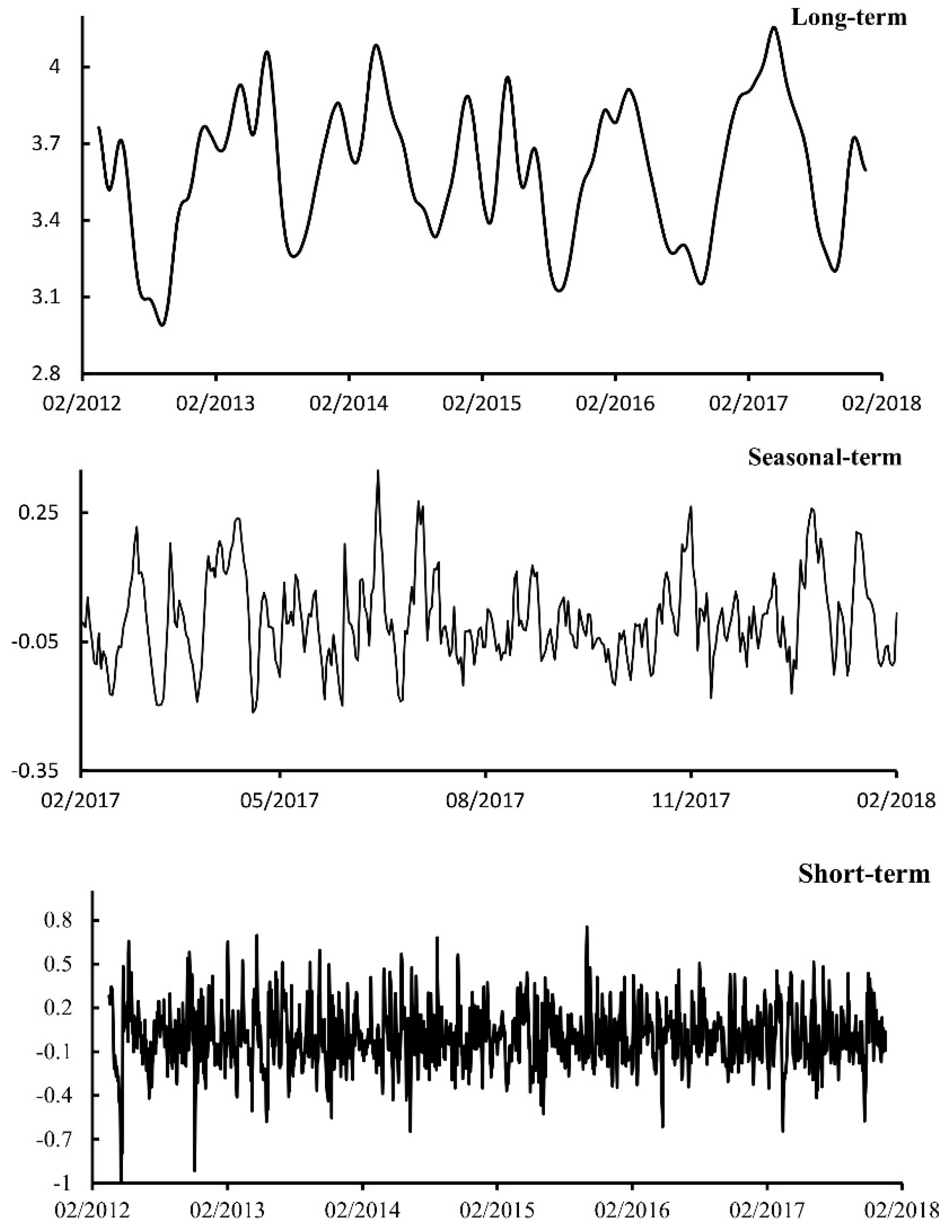
The forecasting accuracy of the data has been improved by separating the different cycles on the raw data using the time series decomposition (long, seasonal, and short-term component) as described in
Figure 5.
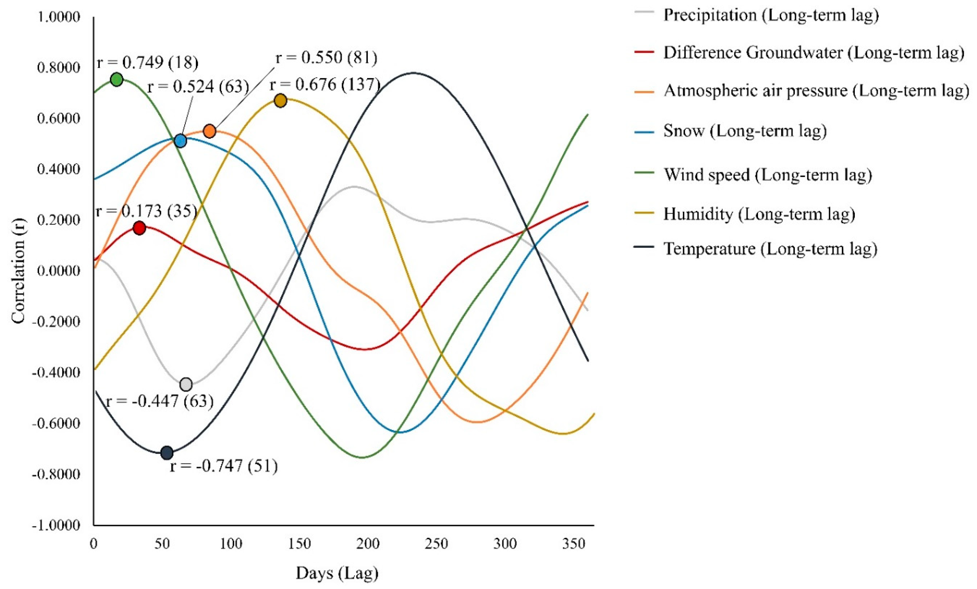
For the prediction of the long-term component of the water discharge time series, the lagged-variables wind speed, atmospheric air pressure, snow, humidity, and difference groundwater provide a positive correlation (
Figure 6). The lagged-precipitation provides a negative correlation of −0.45 with the water discharge that occurs at the minimum value of the curve (
Figure 6). The atmospheric air pressure has shown a substantial improvement in the correlation from 0.02 to 0.55 which has been occurred at the lag of 81-days. A similar improvement was observed for the precipitation. The correlation has been increased from 0.05 to 0.45 at the lag of 63-days. A moderate improvement has been noticed for the 137-days lag of humidity by reversing the negative correlation to positive, and for the snow depth at the 63-days lag. A lower improvement has been noticed with the variables wind speed and difference in groundwater.
Using the appropriate lags for the predictor variables, the TSR model for the long-term component has been designed with Equation (9):
R2 = 0.93.
The predictor variables in Equation (9) are statistically significant, and there is no collinearity between the variables (
Table 2). The coefficient of determination (R
2) derived from the TSR model is equal with 0.93, which implies that the climatic and hydrogeological variables can explain 93% of the variance in the water discharge. In case that the MLR model is used for the prediction of the long-term component in the water discharge, the coefficient of determination is 0.74 (
Table 3).
Using the MLR model the unexplained part of the prediction of the long-term component of the water discharge is 26% while using the TSR model the unexplained part of the prediction of the water discharge is 7%. Thus, using the TSR model for the prediction of the water discharge, we improve the explanation of the long-term approximately four times.
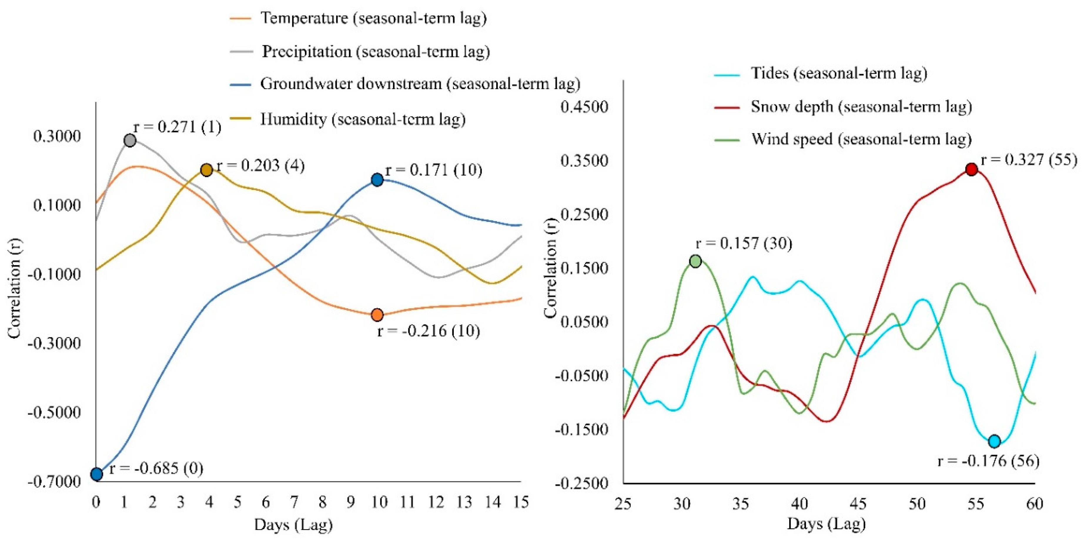
Selection of the appropriate lagged-variables for the seasonal component has improved the prediction of the water discharge using the predictor variables. The correlation coefficients are estimated between the variables (
Table 3). Precipitation, humidity, groundwater downstream, snow depth, and wind speed indicate a weak positive correlation with the seasonal component of the water discharge time series (maximum points on the curve in
Figure 7). Temperature and tides indicate a weak negative correlation with the seasonal component of the water discharge data (minimum points on the curve in
Figure 7). The maximum points on the curve indicate the best correlation value to the dependent variable (water discharge). The seasonal-term was split into two different time components because the data indicated short lag values with the best correlation and long lag values with the best correlation. The current value of the groundwater downstream shows a strong negative correlation and the lagged by ten days groundwater downstream shows a weak positive correlation. Both groundwater downstream variables contribute to the seasonal component of the TSR model with no collinearity effect. A similar effect has been concluded for the temperature variable, as well. In particular, the current value of temperature shows a positive correlation with the water discharge and the lagged by ten days temperature shows a negative correlation. Both temperature variables have been used in the TSR model with no collinearity effect. Based on
Figure 7, the lag operator that has been applied in the predictor variables to maximize the correlation with the seasonal component of the water discharge data has shown a poor improvement of the correlation (r) values with a maximum correlation at around 0.32 (by the snow depth) and a mode value of all the correlations (r) from the lagged variables at about 0.2.
The TSR model has been applied in the seasonal components of the variables with statistical significant coefficients in the model and no collinearity effect between the predictor variables (
Table 4). Using the lag operator in the predictor variables as described on
Figure 7, the prediction of the seasonal component of the water discharge data can be expressed by:
R2 = 0.58.
The coefficient of determination (R
2) for the TSR model is equal with 0.58. In case that the MLR model will be used for the prediction of the seasonal component of the water discharge data, the coefficient of determination is equal with 0.50 (
Table 3). Therefore, there is an 8% improvement in the prediction of the seasonal component of the water discharge data using the TSR model.
The prediction of the short-term component of the water discharge was estimated using the same methodology, and the temperature, tides, precipitation, and humidity variables indicate a positive correlation with the water discharge data, while the atmospheric air pressure has shown a negative correlation (
Figure 8). In particular, humidity can be transformed with a 4-days lag, atmospheric air pressure with a 3-days lag, temperature and tides with a 2-days lag. Precipitation denotes a 1-day lag with the short-term component of the water discharge data. The correlation improvement is weak in the short-term component and did not exceed the correlation value of 0.33 which corresponds to the lagged precipitation variable. Correlation values for all lagged variables drop at the 5th-day of lag with a correlation value of less than 0.1, while they decrease to less than 0.05 after the 14th-day of lag. Using the lag operator on the temperature, tides, precipitation, atmospheric pressure and humidity data, the TSR model has been applied in the hydrogeological and climatic variables and can be described by Equation (11):
R2 = 0.41.
The coefficients in the model used in Equation (11) are statistically significant, and the predictor variables do not indicate any collinearity (
Table 4). The TSR model for the short-term components has a performance of 41% (R
2). In case that the MLR model (no lags are considered in the model) is applied in the short-term component of the hydrogeological and climatic variables, the performance of the model is 29% (
Table 3). The improvement of the flood prediction model is 12%. Using the MLR model the unexplained part is 71% while using the TSR model the unexplained part is 59%. Therefore, using the lag operator, the prediction of the short-term component has been improved approximately by 1.2 times.
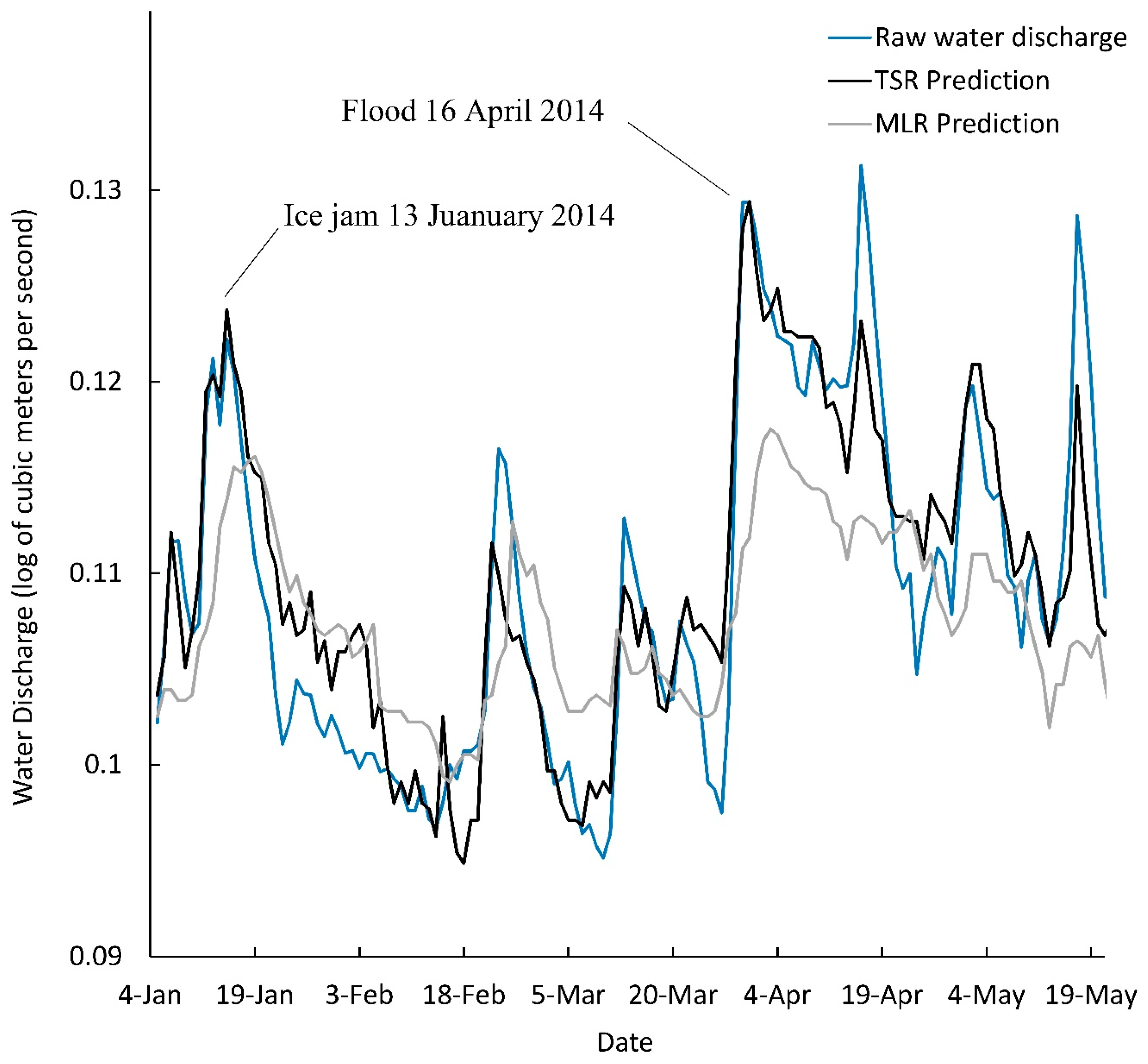
Combining the Equations (9)–(11) we provide the TSR prediction model for the water discharge time series. An example of the prediction model is presented in
Figure 9 for the water discharge date measured from 4 January 2014 to 19 May 2014. The raw water discharge data, the predicted TSR model of the water discharge, and the predicted MLR model of the water discharge data are presented in
Figure 9. The TSR prediction model shows an improved prediction with an example of the successful predicted flood on 13 January 2014 and on 16 April 2014. The flood event on 13 January 2014 has been occurred due to the ice jam in Mohawk River, New York [
33], and the flood event on 16 April 2014 has been occurred due to ice melt in Mohawk River. Both floods were observed by the USGS monitoring station with a substantial rise in the water discharge. We present the prediction of the water discharge using the TSR and MLR models during the above periods (
Figure 9). The TSR model performs well and successfully reproduces the two flood events, unlike the MLR model barely overlaps the peaks of the water discharge rise.
The overall performance of the TSR model is 73.22% and describes the total explanation of the water discharge data by using the hydrogeological and climatic variables (
Table 5). In particular, using the TSR model the hydrogeological and climatic variables explain 73.22% of the variance of the raw water discharge.
6. Discussion
The hydrologic cycle is a complex system that involves the contribution and interferences of different climatic and hydrogeological variables. To issue a flood forecasting, all available variables should be decomposed to avoid interferences and provide a meaningful physical interpretation. Time series decomposition is a powerful statistical technique that scales large and complex systems. It facilitates numerical modeling to separate components from the variable’s integration and orchestration. In this study, we use the time series decomposition and the lag operator to increase the power of the prediction model compared to the prediction of the raw data. In particular, we use two different transformations (the lag operator and the time series decomposition) to minimize the collinearity between the variables. The Kolmogorov-Zurbenko filter has been used for the time series decomposition, and the lag operator has been applied in the predictor variables of the time series regression model. Combining both operators, we improve the explanation of the model for the prediction of the water discharge data. In particular, the unexplained part of the raw data is approximately 50% (
Table 5) while the unexplained part of the combined time series regression model for the decomposed data is approximately 25% (
Table 6). Thus, using both statistical techniques, we improve the prediction of the water discharge approximately two times.
The TSR model provides a higher forecasting performance compared to the MLR model. With the TSR, the lag operator has been applied in the predictor variables, and different time-lags have been considered in the model for the prediction of the long, seasonal, and short-term component of the water discharge time series. The time lags that have been selected for the predictor variables provide a physical interpretation of the data and provide the strongest correlation with the water discharge time series. The TSR is a dynamic model compared to the MLR model and provides the advantage of considering past values for the hydrogeological and climatic variables. Also, using the MLR model, essential variables such as precipitation “loses” the correlation with the water discharge because we do not account any lag in the model, and we lose information including the physical interpretation. In the selected TSR model the lagged predictor variables have been selected to sustain their independence.
For the prediction of the water discharge data, the lag operator that has been applied to the predictor variables depends on the component of the time series (long, seasonal, and short-term component). In particular, smaller values of lags have been used for the prediction of the short-term component of the water discharge while larger values of lags have been used for the prediction of the long and seasonal components. This is because the short-term component describes the short-term variations and the contribution of the climatic and hydrogeological variables is stronger for the smaller values of the lag operator. Contradictory, the long and seasonal-component describe the year-to-year fluctuations or variations greater than a given threshold. Thus, the relationship between the water discharge and the predictor variables is stronger for larger values of the lag operator. In case that we use the lag operator in the raw data, there is no substantial contribution of the lagged predictor variables for the explanation of the water discharge time series due to the mixed frequencies on the time series data. Collinearity test in the raw variables using the lag operator has failed, implying that the raw data require decomposition due to the interferences between the different frequencies in the time series. The decomposed time series permit efficient participation of the lagged-variables in the TSR model because they do not show collinearity and interferences between the lagged-variables.
Using the lag operator in the time series regression model, we can reveal the true relationship between the water discharge and the hydrological and climatic variables. Correlations between the water discharge and the predictor variables that are very weak (positive or negative) have been transformed to a strong positive or negative relationship when the lag operator has been applied in the climatic and hydrogeological variables due to a time delay. This time delay between the water discharge and the predictor variables has been revealed at different time scales with the decomposition of the time series. The time lag varies depending on the time series component of the water discharge (long, seasonal, and short-term component). In the long-term component, the delay varies from 18 to 137 days, in the seasonal component from 1 to 56 days, and in the short-component from 1 to 4 days.
6.1. Physical Interpretation
The advantage of the TSR model is the capability of integrating most of the lagged-variables. In particular, using the collinearity test and the statistical significance of the predictor variables we include most of the lagged-variables in the TSR model. The long-term component of the lagged wind speed variable is one of the variables that although was statistically significant in the TSR model, it was not possible to be physically interpreted, however, we think that is related to a local climatic effect. The lagged-variables and their correlations with the water discharge revealed several patterns. The strongest correlation between the lagged-variables with the water discharge may reveal the critical value at which high-risk flood may take place because the lagged-variable will show a peak-contribution to the water discharge rise. The reverse correlation (from positive to negative and vice versa) between the water discharge and the lagged-variables is prominent in some variables (
Figure 6), and a resulted physical interpretation is possible. High lag values at long and seasonal components facilitate a physical interpretation of the hydrogeological and climatic variables due to the seasons’ transition presence. In the short-term component, a physical explanation is not prominent due to the short lag values that perhaps may correlate to human contribution such as an unscheduled operation of the lock stations, dewatering actions prior to foundations, irrigation, and water supply to the surrounding towns.
6.2. Large Lag Values
In the long-term components, we expect to identify large lag values due to the large periodicities that sometimes reverse their correlation. At higher lag values the negative correlation between the water discharge and the humidity reverses to a positive correlation. The inverse relationship exists with the water discharge at lag-1 day with a moderate negative correlation (r = −0.38), while at lag-137 there is a strong positive correlation (r = 0.68). At the first 55-days, the long-term lagged-variable of humidity indicates a decreasing negative correlation with the water discharge. A possible local weather effect such as intensive evaporation from the watershed may dissipate during this 55-days of humidity in the summer season which contributes to increasing humidity while the water discharge decreases. In the fall season, the negative correlation has been reversed to a positive correlation, and an intensive rainfall and a subsequent aquifer recharge may increase the water discharge. The contribution of the humidity to the water discharge will peak at 137-days showing the strongest correlation. Selecting data cases such as summer and winter periods has shown that a substantial difference in correlation exists between the water discharge and the humidity. This correlation is approximately five times (r = 0.63) stronger in the summer than the winter season. In the winter, during low humidity days when river freezes and permeability decreases, the snow accumulation usually occurs and water discharge decreases. As the long-term humidity precedes the water discharge by 137 days, high humidity values may imply high-risk of a flood at approximately four months later.
The pressure shows a lag of 81-days providing a significant correlation with the water discharge. It is possible that a luni-groundwater correlation might exist, that is the number of lunar revolutions with the groundwater response which subsequently affects the water discharge. Considering that a lunar revolution is around 27-days, then the 81-days coincides with approximately 3 lunar cycles. It may reveal a relation to a luni-groundwater correlation.
In the long-term, the snow lagged-variable of 63-days shows the strongest positive correlation (r = 0.52) while 5-months later the lag of 223 days variable reverses the correlation to the strongest negative (r = −0.63). The positive correlation at the lag of 63-days implies that after a snow-storm at approximately the 63-day the water discharge will have the strongest contribution from the snow accumulation due to the recharge of the aquifer. At approximately 223-days from the first snow-storm, the water discharge will show the lowest value which will be in the summer.
At a similar time of 56-days and 233-days, the long-term of temperature with moderate correlation (r = −0.5) shows a similar pattern of correlation variation. The negative strongest correlation (r = −0.75) occurs at 52-days lag, while the positive strongest correlation (r = 0.75) occurs at 233-days lag. Unfortunately, the lagged temperature is not independent with the remaining lagged predictor variables, and due to collinearity, there is no integration of this variable in the TSR model of the long-term components described by Equation (9).
The variable of the difference between the two groundwater stations (GWDIF) also shows a similar pattern of moderate correlation and subsequent fluctuation. There is no correlation (r = 0.04) with the non-lagged variable of the GWDIF at 0-days, while the lagged-variables at 40-days (r = 0.17) and 200-days (r = −0.31) show reversing correlation. The downstream and upstream groundwater stations (GWD, GWU) show a very strong correlation with the water discharge and a similar pattern of correlation fluctuation. However, the collinearity test did not permit the utilization of any of those two groundwater stations to be integrated into the TSR model (Equation (9)). Implementing a different TSR utilizing the temperature and the groundwater lagged-variables yields a lower correlation (r < 0.8) and subsequent forecasting performance than the chosen long-term TSR model (r = 0.96).
6.3. Short Lag Values
In the short-term components, the lag operators range from 1 to 4 days to improve the power of the prediction model. Although most of the variables in the short-term show a positive correlation with the water discharge, the atmospheric air pressure is the only variable that shows an inverse relationship with an increasing lag time. The short-term humidity shows an improvement of a positive correlation with the water discharge at the 4th-day lag. After the 5-day lag, the correlation between the predictor variables and the water discharge drops to less than 0.1. Also, after the lag of 12-days, the correlation becomes less than 0.05 or approximately zero, implying the successful decomposition of the time series as it indicates very short lags that do not exceed the four days period. There is no evidence of any long-term or seasonal-term cycle in the short-term component, and the time series components are uncorrelated which implies a successful decomposition.
Schenectady County has variable permeability with mostly high-permeability layers overlain by low-permeability layers, a variable water-infiltration potential of the soil zone [
37,
38], and a small aquifer. The 65 km
2-valley-fill aquifer with quaternary deposits covers a small portion of the Mohawk Watershed. The Schenectady County permeability is an important factor that may contribute to the lag time that the aquifer requires to discharge or replenish. Despite the permeability influence, the volume of the aquifer may affect the discharge or recharge rate. A small aquifer requires less time to replenish or discharge, and the short-term should reflect the groundwater contribution to the water discharge. A hypothesis of a small aquifer with shallow low-permeability layers on the surface of Schenectady County may not facilitate the water infiltration, and it may require a longer time to recharge the aquifer. The groundwater may not respond to a short-term increase from the precipitation, and the runoff water will significantly contribute to the water recharge short-term rise. We noticed that there is no lagged-groundwater contribution to the short-term component of the water discharge which confirms the above hypothesis and flood risk from a flash flood or ice jam increases.
6.4. Collinearity and Correlation Values
A rivalry between the correlation and the collinearity test values exist in the lag values that may not permit the selection of some variables even though the correlation is strong in various lag values. Although the long and the short-term show substantial improvement with the integration of the lagged-variables, the seasonal-term component does not show a prominent enhancement as the correlation coefficient with the lagged-variables does not exceed the value of 0.2. The short-term and the long-term component have shown a series of lag values that as the lag value increases, the correlation with the water discharge weakens. The seasonal-term did not show any pattern. For the seasonal lagged tide variable, as the lag value increases the VIF value decreases permitting the integration of this variable in the model. Thus, we select a peak correlation at 56-day lag which is two full revolutions of the Moon around Earth (sidereal month is equal to 27.3 days).


