Using Historical Precipitation Patterns to Forecast Daily Extremes of Rainfall for the Coming Decades in Naples (Italy)

Abstract

The coasts of the Italian peninsula have been recently affected by frequent damaging hydrological events driven by intense rainfall and deluges. The internal climatic mechanisms driving rainfall variability that generate these hydrological events in the Mediterranean are not fully understood. We investigated the simulation skill of a soft-computing approach to forecast extreme rainfalls in Naples (Italy). An annual series of daily maximum rainfall spanning the period between 1866 and 2016 was used for the design of ensemble projections in order to understand and quantify the uncertainty associated with interannual to interdecadal predictability. A predictable structure was first provided, and then elaborated by exponential smoothing for the purposes of training, validation, and forecast. For the time horizon between 2017 and 2066, the projections indicate a weak increase of daily maximum rainfalls, followed by almost the same pace as it was in the previous three decades, presenting remarkable wavelike variations with durations of more than one year. The forecasted pattern is coupled with variations attributed to internal climate modes, such as the Atlantic Multidecadal Oscillation (AMO) and the Pacific Decadal Oscillation (PDO).

1. Introduction

Precipitation patterns indicate an increased frequency and intensity of extremes over mid-latitude land areas (20–50° N), with especially rapid changes since the 1990s [1]. The amount of precipitation on very wet days (exceeding the 95th percentile) has increased worldwide from about 160 mm to 185 mm (Figure 1, modified from Cohen et al. [1]). Precipitation patterns are also a consistent feature in future projections from coupled climate models forced with increasing greenhouse gas (GHG) atmospheric concentrations (e.g., [2]). These projections can be different based on a variety of Global Climate Models (GCMs) [3,4,5,6] and the different parameter sets involved in the simulations under alternative GHG emission scenarios. Results from data-driven models corroborated the results by GCM projections [7,8,9]. However, the ability of the GCMs to reproduce future climate has often been questioned [10,11,12,13,14,15,16]. In particular, extreme events may be difficult to predict because they are characterized by a large uncertainty in the occurrence time and the magnitude of the event [17].

Simulating site-specific extreme rainfalls is needed as a basis for understanding ecosystem and landscape responses, studying environmental planning, and for other water supply-related issues. Applying soft-computing forecasting is claimed given the large investments being made in modelling strategies, which are computationally demanding (due to the requirement to run multiple realisations), typically require access to high-performance computing clusters, and are unlikely to avoid high levels of uncertainty in the estimates [18]. Leith [19] used the fluctuation-dissipation (F-D) theorem from statistical mechanics, implying that the use of complex models are not necessarily getting any better future projections than simple statistical models.

There are several methods for predicting complex time series [20]. Exponential Smoothing (ES) considers a set of data stretching back infinitely far into the past. It considers smaller weights for older data points as new data points are added, and thus older data points have successively less impact on estimates as time goes on. Exponential smoothing [21] and Autoregressive Integrated Moving Average (ARIMA) models [22] are the most representative methods in time series analysis. We used ES for its advantages against ARIMA models: (i) it is optimal for a broader class of state-space models [23]; (ii) it easily responds to changes in the pattern of time series [24]; (iii) it is often referred to as a reference model for time–pattern propagation into the future [25,26]; (iv) it is less complex in its formulation and thus easier in identifying the causes of unexpected results [27]; and (v) it tends to be more robust with non-stationary time series [28]. For the town of Naples (Italy), we developed an Exponential Smoothing Approach (ESA) to explore the Annual Daily Maximum Rainfall (ADMR) series, under the assumption that the past interannual climate variability, with its internal dependence structure, can be used to replicate future intensive rainfall ramification at the local scale. For the town of Naples, there is now an accessible accurate long-time series of ADMR (1866–2016). Our focus on this town is motivated because in its region, extreme rainfalls tend to produce multiple damaging hydrological events, such as flash floods, urban landslides, and sediment transport (e.g., [29]), as also reported in historical sources [30]).

2. Materials and Methods

2.1. Study Site and Data Sources

The Naples weather observatory (40°50′ N, 14°15′ E) is placed over the highest part of city, at 150 m a.s.l. The climate in the area is characterized by mild seasons with more thermal contrast in autumn, when the sea is still warm and flows of fresh air can come from the North Atlantic or the east. Especially in this season, intense and very erosive rainfalls can occur, although winter and spring are both frequently crossed by depressions generating over the Mediterranean Sea [31]. The earliest regular instrumental observations started in Naples in 1821 at the Capodimonte Astronomical Observatory (http://www.na.astro.it), when rainfall readings were recorded by an ordinary pluviometer and a Richard’s pluviograph until 1950. Successively, the measurements continued to the near Capodimonte observatory and recently (in the year 2000), the observatory was included in the hydropluviometric network of the Civil Protection of the Campania Region (http://www.amracenter.com/en/projects/civil-protection-of-the-campania-region.html). Daily rainfalls are available only from 1866 forward.

Before undertaking a modelling work on the ADMR series, an exploratory analysis was performed for inhomogeneity detection (when a series is homogeneous, its values tend to fluctuate around their mean, because no significant deviations of the values with respect to their mean appear). In fact, since hydrological records such as daily and annual rainfall are of a chaotic nature in time and space (with limited or any autocorrelation structure in a time series), the rainfall processes appear as discontinuous phenomena that rarely assume the form of an internal autocorrelation, especially at short time lags. In a climatic time series of this type, inhomogeneities are not rare, because non-climatic factors can cause discontinuities, which may hide climate signals and patterns.

To forecast the upcoming values of rainfall extremes based on their historical sequence, the online freeware application Smooth Forecast [32] was used, which provides free time series forecasting capability on the web. It allows specifying a “hold back” number of values off the end of the history, and thus the system forecast is based upon the history prior to the held back values. The length of the out-of-sample (validation) period is dependent on the forecasting goal, data frequency, and forecast horizon. Typically, the validation period mimics the forecast horizon to allow the evaluation of actual predictive performance. With a shorter period than the forecasting horizon, the predictive performance of long-term forecasts is not assessed. If the validation period is longer than the forecast horizon, then the training period will have less recent information. The system compares the forecast with the held back history and produces metrics that can be used to assess the accuracy of the forecast. With the support of a spreadsheet, the statistics were assessed interactively using statistics software WESSA R–JAVA web [33]. Using the Java-based software tool SELFIS (SELF-similarity analysis, [34]), we estimated the Hurst (H) exponent (rate of chaos), which quantifies long-range dependence and appraises possible cyclical-trend patterns in the series: 0.5 < H < 1.0 indicates positive memory (past trends tend to persist in the future); 0.0 < H < 0.5 indicates negative memory (past trends tend to revert in the future).

2.2. Statistical Model

One of the simplest and most popular forecast equations is exponential smoothing, which is a simple prototype for all time series-based forecasting equations [35]. This technique uses historical, or time-series data under the assumption that the future of the series will be similar to the past; it attempts to identify specific patterns in the data and project and extrapolate those patterns into the future without trying to identify the causes of the patterns. In this way, a periodically multiplicative exponential smoothing with no trend [26] was selected as the reference model for time-pattern propagation into the future:

$$F{\left(X\right)}_{t+m}^R=S_t\times I_{t-p}$$

(1)

where $F{\left(X\right)}_{t+m}^R$ represents the m-step ahead forecast from the annual series (y_t) of daily maximum rainfall on N years for ensemble (Rth) run (in this study, 10 runs were launched from different initial conditions); S_t is the daily maximum rainfall at the time-year t:

$$S_t=\alpha \frac{X_t}{I_{t-p}}+\left(1-\alpha \right)\times S_{t-1}$$

(2)

where X_t is the actual daily maximum rainfall in the annual series, and α is the smoothing parameter for the data. The smoothed cycle index (I_t−p) at the end of period t with p periods in the multiyear cycle is iteratively formulated as:

$$I_{t-p}=\delta \frac{X_t}{S{\left(X\right)}_t}+\left(1-\delta \right)\times I_{t-1}$$

(3)

where δ is the smoothing parameter for cyclical indices.

Model performance against the validation period was assessed with the Root Mean Squared Error (RMSE), the Mean Absolute Percentage Error (MAPE), the Mean Absolute Scaled Error (MASE), and the correlation coefficient (R). The RMSE [36] measures the square root of the average squared difference between the values predicted by a model and the values that are actually observed. It provides a measure of how far away the forecasts are from observations. The MAPE is intuitive in terms of relative error (e.g., the prediction model is considered reasonable with a MAPE below 30%, and very accurate with a MAPE less than 10% [37]) and has the advantage of being scale-independent. However, few major outliers in the series can substantially skew the RMSE and MAPE statistics. The MASE is a non-dimensional measure of the accuracy of forecasts [38], which is more robust to outliers than the RMSE and the MAPE. Essentially, it is the average of the absolute scaled forecast, where the scaling factor is determined by using a random walk model (naïve reference model on the history prior to the holdback period). Ideally, a MASE of <1 implies that the forecast model is superior to a random walk. The correlation coefficient R between estimates and observations [39] ranges from −1 (anti-correlation) to 1 (perfect correlation). It assesses linear relationships in which forecasted values show a continuous increase or decrease as actual values increase or decrease, and its magnitude cannot be consistently related to the accuracy of the estimates.

3. Results and Discussion

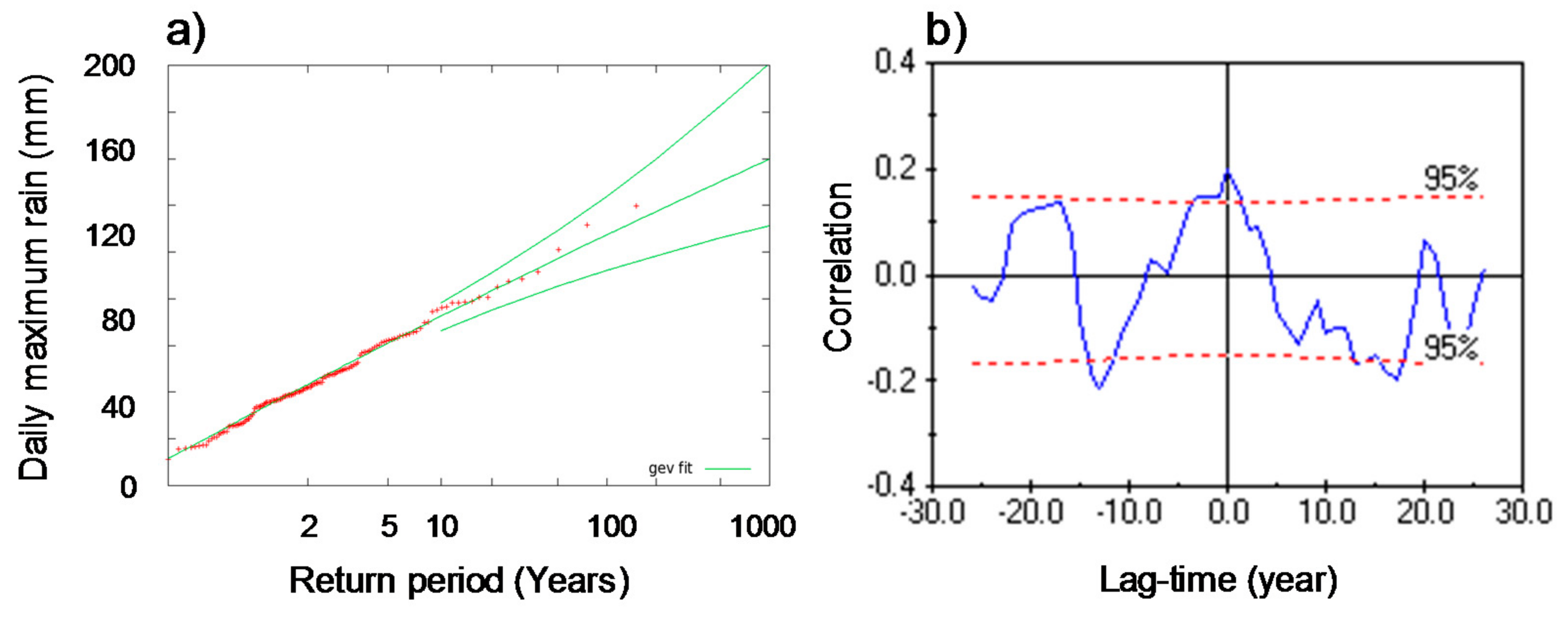
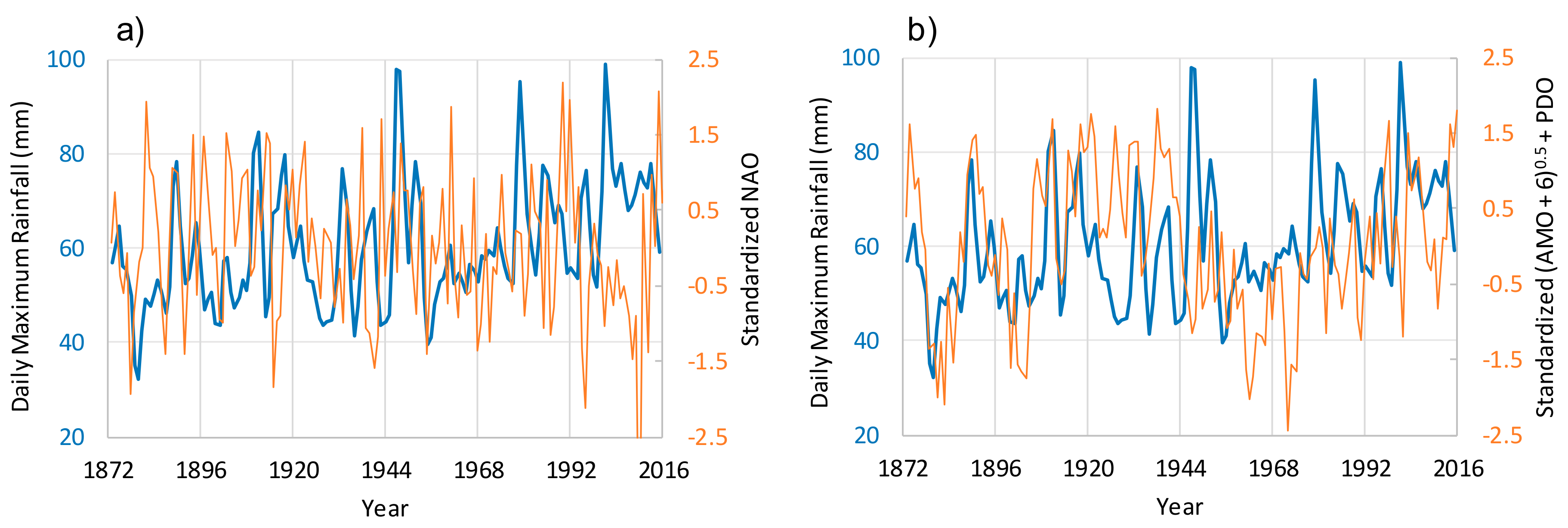
3.1. Exploratory Data Analysis

Our time series does not show significant inhomogeneities, according to the Buishand range test [40], which detects break years in annual data (Figure 2a).

The frequency distribution approximates Gaussian-like distributional features (Figure 2b), while the attractor in the time-state domain shows a ramification towards the diagonal arrow (Figure 2c), which indicates a possible predictable pattern (whether reasonably accurate forecasts can be made).

The Hurst exponent estimated by the R/S method [41,42] is equal to 0.600, which is near the threshold of 0.65 used by Quian and Rasheed [43] to identify a series that can be predicted accurately. However, the Hurst exponent >0.50 indicates that some dependence structure exists, which advocates the foreseeability of the original series.

The model returns a periodical pattern in the extreme rainfall evolution with important cycles equal to 54, which imposes a training period of at least 109 years (as from the software Smooth Forecast). A range of four decades is the maximum allowed for an interdecadal perspective, leaving 111 years available for training (from 1866 to 1976).

3.2. Validation Test

For the validation period between 1977 and 2016 (Figure 3a), the simulation results are quite promising, judging by the overall closeness of the red prediction curve to the blue curve of observed extreme rainfall evolution.

For the validation period, the metric statistics R, RMSE, MAPE, and MASE, which are equal to 0.40, 25 mm, 26.5%, and 0.692, respectively, indicate a satisfactory performance, and imply that the forecast model is superior to a random walk. Model residuals have a quasi-normal distribution (Figure 3b), and the Q-Q (quantile-quantile) plot shows that the theoretical and sample quantiles are quite similar (Figure 3c). Owing to only a few data points, the distribution is slightly right-skewed, rising more slowly at the beginning and then rising at a faster rate for higher values.

Overall, the model provides realistic values on average, but peaks are often not captured. The results thus indicate that the exponential model for rainfall simulation can be employed to reasonably characterize and predict dominant patterns of variability at interannual to interdecadal time scales, while they may not be unambiguously disclosed in short-term (one year ahead or so) forecasting.

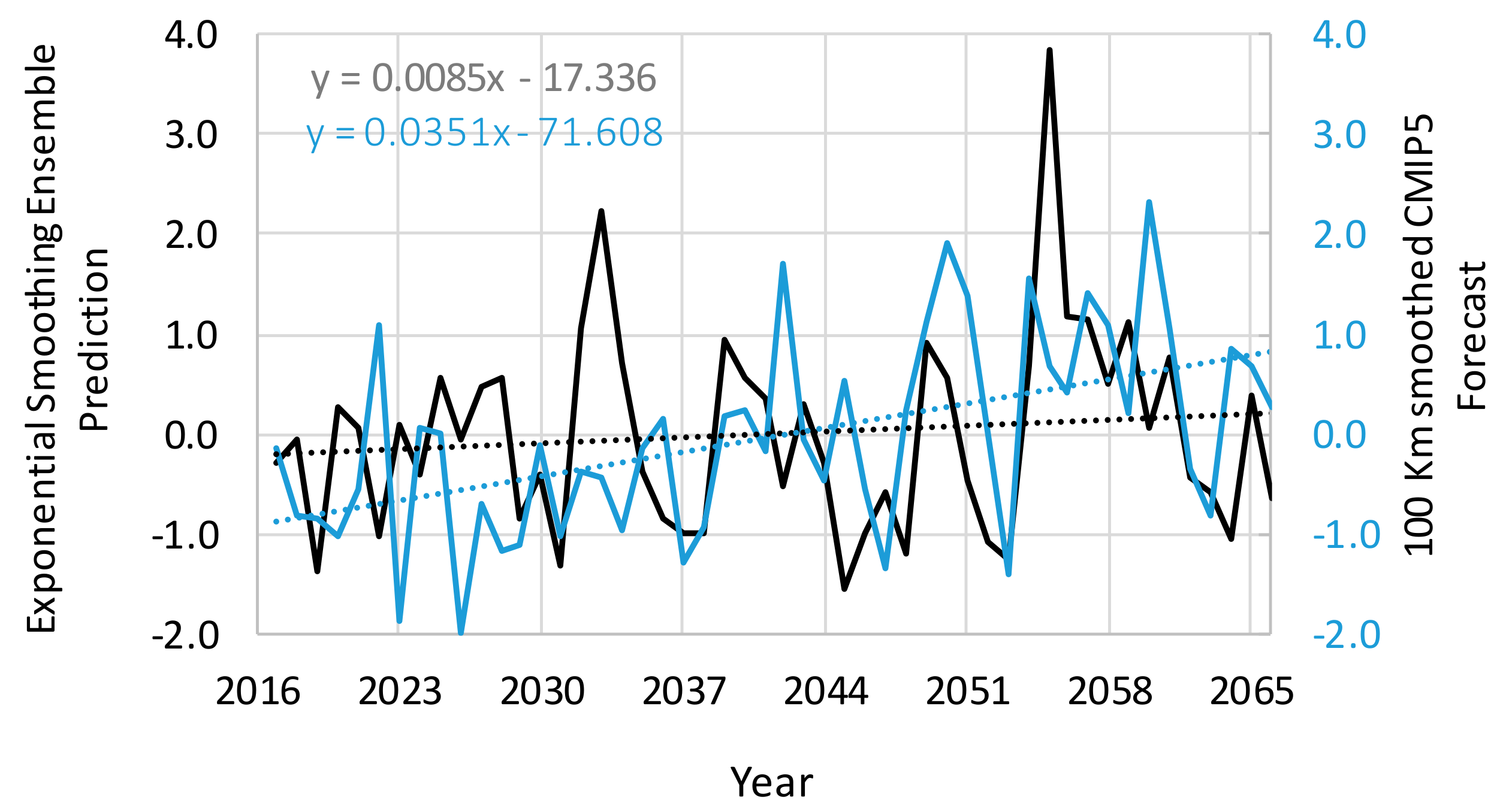
3.3. Simulation Experiment

The ability of the model to extrapolate results is dependent on the stochastic and deterministic behaviours of time-dependent terms. In this specific case, the system appears to evolve as influenced by natural variations, which are also weakly predictable (after Miglietta et al. [44]).

When examining the projection of daily maximum rainfall over the four future decades (2017–2066, Figure 4), the values of the ensemble (black curve) are observed to roughly lie around or above the long-term median (bold grey lines). The plumes band (colour curves) gives an approximate idea of the uncertainty associated with the forecasts. A weak increasing trend is shown (Figure 5), by almost the same pace as it was in the previous three decades.

The extreme value of about 130 mm, corresponding to a 100-year return period (red line), is overstepped one time within the forecasted period. Also, the interdecadal variability is pronounced, with the annual single values often approaching the 10-year return period of 93 mm (orange line), as estimated by GEV (generalized extreme value) distribution (Figure 6a).

The observable trend into the projection is crossed by cyclical patterns that are still present as in the past, with a moderate magnitude around the 2030s and 2050s decades. Figure 4 also displays the oscillation of the mean of the plumes forecast (with peaks after 2050), which encloses the CMIP5 (Coupled Model Intercomparison Project Phase 5) smoothed mean (blue dots). Thus, the latter shows a similarity in the cyclical pattern with our projections. However, the general trend of the CMIP5 output is approaching 0.04 mm yr⁻¹, which is about four times higher than that of the exponential smoothing forecast (Figure 5).

This appears compatible with an intensification of extreme precipitation events during the 21st century, which are attributed to the increasing atmospheric moisture content in a warming climate (according to the Clausius-Clapeyron equation) and projected by GCMs modulated by a range of factors such as temperature lapse rate, vertical wind velocities, and temperature anomalies when extreme events occur [45,46]. These smoothed oscillations may be induced by atmospheric and ocean forcing, such as the Pacific Decadal Oscillation (PDO) and the Atlantic Multidecadal Oscillation (AMO) that act on the hydroclimatic system in multiple ways. Indeed, the studied time series appears to be just cross-correlated with teleconnection indices such as the PDO and AMO (Figure 6b). This cross-correlation supports the predictability of our model, implying that the statistical model would reproduce a coupled oscillation between extreme rainfalls and AMO–PDO indices. Our analysis (Figure 7) does not support a relation between our output (extreme rainfall at Naples, mostly occurring in autumn) and dynamics of the North Atlantic Oscillation (NAO), whose major influence on Italian precipitation (mostly winter precipitation) is documented [47]. Daily maximum rainfall in Naples is only weakly correlated with NAO (Figure 7a), while the combined AMO/PDO index shows a comparable course (Figure 7b). In particular, higher (lower) rainfall maxima tends to coincide with positive (negative) phases of the combined index. Knudsen et al. [48] conjectured that a quasi-persistent ~55-to-70-year AMO, linked to internal ocean–atmosphere variability, existed during large parts of the Holocene, thus suggesting that the coupling of AMO and regional climate conditions was modulated by orbitally-induced shifts in large-scale ocean–atmosphere circulation.

These results suggest an astronomic origin of the ~50-to-70-year variability found in several climatic records [49]. Moreover, the PDO can modulate the interannual relationship between El Niño Southern Oscillation and the global climate, with large dry–wet variations over northern Europe and the Mediterranean [50]. The PDO influence can be transmitted to the Atlantic European region indirectly via the NAO by the mechanism involving a shift of the North Atlantic storm track [51]. In this way, cyclone activity tends to enhance during the positive AMO phases and the negative PDO phases, when the zonal flow is further south.

4. Conclusions

We developed a statistical ensemble forecast approach in an effort to anchor the reality of daily maximum rainfall (annual series) to the changes observed in the past, and replicate these changes in the near future (four decades). A comparison with GCM-based forecasts was also approached that could be looked further at in future analyses of hydrologic extremes. In fact, highlighting the ability of relatively simple statistical approaches (as compared to complex models) is a key issue, which may be against the speculative use of results from forecasting tools.

Based on the analytical framework and concepts discussed in previous papers [52,53], our analysis used a relatively simple soft-exponential smoothing approach for maximum daily rainfall forecasting in Naples (Italy). The results of this study can be useful for predicting and managing extreme hydrological events, and support further predictive studies beyond the use of GCMs. Forecasts over four decades ahead (of the same duration as the validation period) allowed the emergence of interannual to interdecadal patterns. However, the extrapolation of rainfall extremes into the future uses greatly simplified assumptions in most instances, especially in regime shifts and trends, and does not capture many of the complexities and natural variations that dynamically produce hydrologic changes. In fact, lagged variables, autocorrelation, and non-stationarity make time-series forecasting notoriously difficult [54]. The degree of confidence that we place on climate predictions essentially depends on whether we can quantify the uncertainty of the prediction, and demonstrate that the results do not depend strongly on modelling assumptions [55]. Approaches of this type may also suffer from overfitting to past data (conditions occurring randomly within the training periods as part of the internal variability of the climate system), which may lead to unreliable forecasts. In spite of that, the development of decadal predictions in the Mediterranean sector is relevant to both research and decision making, because the multidecadal variability of the large-scale oceanic circulation exerts a significant effect on the precipitation regime in this region (e.g., [6]). Although caution has to be exercised in relating climatological indices to hydroclimatic variables such as hydrologic extremes (which are temporally discontinuous and chaotic), the improvement of decadal climate predictions with statistical tools is to be encouraged. The relationship between an AMO/PDO combined index and the extreme rainfall patterns identified in this study needs to be substantiated beyond our study site. Further evidence substantiating this relationship would permit making reasonable inferences about trends of rainfall extremes in the medium and long-term. That the methods used so far are probably still too simplistic calls for further research into the dynamic causes of observed and simulated decadal variability. We opted for a simpler model than a dynamic approach with chaotic motion, because the limited length of the time series did not allow the application of some more complex models. This paper may help in stimulating the debate about less conventional ways of understanding the climate mechanisms behind hydrologic extremes, without the need for large computational and financial support, as commonly happens when performing climate model simulations.

References

1. Cohen, J.; Screen, J.A.; Furtado, J.C.; Barlow, M.; Whittleston, D.; Coumou, D.; Francis, J.; Dethloff, K.; Entekhabi, D.; Overland, J.; et al. Recent Arctic amplification and extreme mid-latitude weather. Nat. Geosci. 2014, 7, 627–637. [Google Scholar] [CrossRef] [Green Version]
2. Lin, L.; Wang, Z.; Xu, Y.; Fu, Q. Sensitivity of precipitation extremes to radiative forcing of greenhouse gases and aerosols. Geophys. Res. Lett. 2016, 43, 9860–9868. [Google Scholar] [CrossRef]
3. Arnell, N.W.; Delaney, E.K. Adapting to climate change: Public water supply in England and Wales. Clim. Chang. 2006, 78, 227–255. [Google Scholar] [CrossRef]
4. Xu, Y.; Gao, X.; Shen, Y.; Xu, C.; Shi, Y.; Giorgi, F. A daily temperature dataset over China and its application in validating a RCM simulation. Adv. Atmos. Sci. 2009, 26, 763–772. [Google Scholar] [CrossRef] [Green Version]
5. Hazeleger, W.; van den Hurk, B.J.J.M.; Min, E.; van Oldenborgh, G.J.; Petersen, A.C.; Stainforth, D.A.; Vasileiadou, E.; Smith, L.A. Tales of future weather. Nat. Clim. Chang. 2015, 5, 107–113. [Google Scholar] [CrossRef] [Green Version]
6. Dünkeloh, A.; Jacobeit, J. Circulation dynamics of Mediterranean precipitation variability. Int. J. Climatol. 2003, 23, 1843–1866. [Google Scholar] [CrossRef]
7. Triacca, U.; Attanasio, A.; Pasini, A. Anthropogenic global warming hypothesis: Testing its robustness by Granger causality analysis. Environmetrics 2013, 24, 260–268. [Google Scholar] [CrossRef]
8. Mazzocchi, F.; Pasini, A. Climate model pluralism beyond dynamical ensembles. WIREs Clim. Chang. 2017, 8, e477. [Google Scholar] [CrossRef]
9. Pasini, A.; Racca, P.; Amendola, S.; Cartocci, G.; Cassardo, C. Attribution of recent temperature behaviour reassessed by a neural-network method. Sci. Rep. 2017, 7, 17681. [Google Scholar] [CrossRef] [PubMed] [Green Version]
10. Perry, C.A.; Hsu, K.J. Geophysical, archaeological, and historical evidence support a solar-output model for climate change. Proc. Natl. Acad. Sci. USA 2000, 97, 12433–12438. [Google Scholar] [CrossRef] [PubMed] [Green Version]
11. Smith, T.S.; Karl, T.R.; Reynolds, R.W. How accurate are climate simulations? Science 2002, 296, 483–484. [Google Scholar] [CrossRef] [PubMed]
12. Weaver, A.J.; Hillaire-Marcel, C. Global warming and the next ice age. Science 2004, 304, 400–402. [Google Scholar] [CrossRef] [PubMed]
13. Roe, G.H.; Baker, M.B. Why is climate sensitivity so unpredictable? Science 2007, 318, 629–631. [Google Scholar] [CrossRef] [PubMed]
14. Knutti, R.; Krähenmann, S.; Frame, D.J.; Allen, M.R. Comment on “Heat capacity, time constant, and sensitivity of Earth’s climate system” by S.E. Schwartz. J. Geophys. Res. 2008, 113, D15103. [Google Scholar] [CrossRef]
15. Trenberth, K.E.; Fasullo, J.T. Tracking Earth’s energy. Science 2010, 328, 316–317. [Google Scholar] [CrossRef] [PubMed]
16. Furtado, J.C.; Di Lorenzo, E.; Schneider, N.; Bond, N.A. North Pacific decadal variability and climate change in the IPCC AR4 models. J. Clim. 2011, 24, 3049–3067. [Google Scholar] [CrossRef]
17. Zhang, X.; Zwiers, F.W.; Li, G.; Wan, H.; Cannon, A.J. Complexity in estimating past and future extreme short-duration rainfall. Nat. Geosci. 2017, 10, 255–259. [Google Scholar] [CrossRef]
18. Stroe-Kunold, E.; Stadnytska, T.; Werner, J.; Braun, S. Estimating long-range dependence in time series: An evaluation of estimators implemented in R. Behav. Res. Meth. 2009, 41, 909–923. [Google Scholar] [CrossRef] [PubMed] [Green Version]
19. Leith, C. Climate response and fluctuation-dissipation. J. Atmos. Sci. 1975, 32, 2022–2026. [Google Scholar] [CrossRef]
20. Newbold, P.; Granger, C.W.J. Experience with forecasting univariate time series and the combination of forecasts. J. R. Stat. Soc. Ser. A 1974, 137, 131–146. [Google Scholar] [CrossRef]
21. Holt, C.C. Forecasting seasonals and trends by exponentially weighted moving averages. Int. J. Forecast. 2004, 20, 5–10. [Google Scholar] [CrossRef]
22. Box, G.E.P.; Jenkins, G.M. Time Series Analysis: Forecasting and Control; Holden Day: San Francisco, CA, USA, 1976. [Google Scholar]
23. Gardner, E.S., Jr. Exponential smoothing: The state of the art—Part II. Int. J. Forecast. 2006, 22, 637–666. [Google Scholar] [CrossRef]
24. McClain, J.O. Dynamics of exponential smoothing with trend and seasonal terms. Manag. Sci. 1974, 20, 1300–1304. [Google Scholar] [CrossRef]
25. Taylor, J.W. Exponential smoothing with a damped multiplicative trend. Int. J. Forecast. 2003, 19, 715–725. [Google Scholar] [CrossRef] [Green Version]
26. Hyndman, R.J.; Koehler, A.B.; Ord, J.K.; Snyder, R.D. Forecasting with Exponential Smoothing: The State Space Approach; Springer: Berlin, Germany, 2008. [Google Scholar]
27. Crevits, R.; Croux, C. Forecasting Using Robust Exponential Smoothing with Damped Trend and Seasonal Components; Working Papers Department of Decision Sciences and Information Management 588812; Faculty of Economics and Business, Department of Decision Sciences and Information Management: Leuven, Belgium, 2017. [Google Scholar]
28. Monfared, M.A.S.; Ghandali, R.; Esmaeili, M. A new adaptive exponential smoothing method for non-stationary time series with level shifts. J. Ind. Eng. Int. 2014, 10, 209–216. [Google Scholar] [CrossRef]
29. Vennari, C.; Parise, M.; Santangelo, N.; Santo, A. A database on flash flood events in Campania, southern Italy, with an evaluation of their spatial and temporal distribution. Nat. Hazards Earth Syst. Sci. 2016, 16, 2485–2500. [Google Scholar] [CrossRef] [Green Version]
30. Henfrey, A. The Vegetation of Europe: Its Conditions and Causes; J. van Voorst: London, UK, 1852. [Google Scholar]
31. Wigley, T.M.L. Future climate of the Mediterranean Basin with particular emphasis in changes in precipitation. In Climate Change in the Mediterranean; Jeftic, L., Milliman, J.D., Sestini, G., Eds.; Edward Arnold: London, UK, 1992; pp. 15–44. [Google Scholar]
32. Smooth Forecast. Available online: http://smoothforecast.com (accessed on 5 August 2018).
33. Wessa, P. Free Statistics Software, Office for Research Development and Education. version 1.1.23-r7. 2012. Available online: https://www.wessa.net (accessed on 5 August 2018).
34. Karagiannis, T.; Faloutsos, M.; Molle, M. A user-friendly self-similarity analysis tool. ACM SIGCOMM Comput. Commun. Rev. 2003, 33, 81–93. [Google Scholar] [CrossRef]
35. Montgomery, D.C.; Jennings, C.L.; Kulahci, M. Introduction to Time Series Analysis and Forecasting; Wiley: New York, NY, USA, 2008. [Google Scholar]
36. Fox, D.G. Judging air quality model performance: A summary of the AMS workshop on dispersion models performance. Bull. Am. Meteorol. Soc. 1981, 62, 599–609. [Google Scholar] [CrossRef]
37. Nor, N.I.A.; Harun, S.; Kassim, A.H.M. Radial basis function modeling of hourly streamflow hydrograph. J. Hydrol. Eng. 2007, 12, 113–123. [Google Scholar] [CrossRef]
38. Hyndman, R.J.; Koehler, A.B. Another look at measures of forecast accuracy. Int. J. Forecast. 2006, 22, 679–688. [Google Scholar] [CrossRef] [Green Version]
39. Addiscott, T.M.; Whitmore, A.P. Computer-simulation of changes in soil mineral nitrogen and crop nitrogen during autumn, winter and spring. J. Agric. Sci. 1987, 109, 141–157. [Google Scholar] [CrossRef]
40. Buishand, T.A. Some methods for testing homogeneity of rainfall records. J. Hydrol. 1982, 58, 11–27. [Google Scholar] [CrossRef]
41. Jens, F. Fractals; Plenum Press: New York, NY, USA, 1988. [Google Scholar]
42. Kamruzzaman, M.; Beecham, S.; Metcalfe, A.V. Non-stationarity in rainfall and temperature in the Murray Darling Basin. Hydrol. Process. 2010, 25, 1659–1675. [Google Scholar] [CrossRef]
43. Quian, B.; Rasheed, K. Hurst exponent and financial market predictability. In Proceedings of the 2nd IASTED International Conference on Financial Engineering and Applications, Cambridge, MA, USA, 8–11 November 2004; pp. 203–209. [Google Scholar]
44. Miglietta, M.M.; Mazon, J.; Motola, V.; Pasini, V. Effect of a positive Sea Surface Temperature anomaly on a Mediterranean tornadic supercell. Sci. Rep. 2017, 7, 12828. [Google Scholar] [CrossRef] [PubMed]
45. Foley, A.M. Uncertainty in regional climate modelling: A review. Prog. Phys. Geogr. 2010, 34, 647–670. [Google Scholar] [CrossRef]
46. Pfahl, S.; O’Gorman, P.A.; Fischer, E.M. Understanding the regional pattern of projected future changes in extreme precipitation. Nat. Clim. Chang. 2017, 7, 423–427. [Google Scholar] [CrossRef]
47. Pasini, A.; Langone, R. Attribution of precipitation changes on a regional scale by neural network modeling: A case study. Water 2010, 2, 321–332. [Google Scholar] [CrossRef]
48. Knudsen, M.F.; Seidenkrantz, M.-S.; Jacobsen, B.H.; Kuijpers, A. Tracking the Atlantic Multidecadal Oscillation through the last 8000 years. Nat. Commun. 2011, 2, 178. [Google Scholar] [CrossRef] [PubMed]
49. Scafetta, N. Empirical evidence for a celestial origin of the climate oscillations and its implications. J. Atmos. Terr. Phys. 2010, 72, 951–970. [Google Scholar] [CrossRef]
50. Wang, S.; Huang, J.; He, Y.; Guan, Y. Combined effects of the Pacific Decadal Oscillation and El Niño-Southern Oscillation on global land dry-wet changes. Sci. Rep. 2014, 4, 6651. [Google Scholar] [CrossRef] [PubMed]
51. Maslova, V.N.; Voskresenskaya, E.N.; Maslova, A.S.L. Multidecadal change of winter cyclonic activity in the Mediterranean associated with AMO and PDO. Terr. Atmos. Ocean. Sci. 2017, 6, 965–977. [Google Scholar] [CrossRef]
52. Diodato, N.; Bellocchi, G. Long-term winter temperatures in central Mediterranean: Forecast skill of an ensemble statistical model. Theor. Appl. Climatol. 2014, 116, 131–146. [Google Scholar] [CrossRef]
53. Diodato, N.; Bellocchi, G.; Fiorillo, F.; Ventafridda, G. Case study for investigating groundwater and the future of mountain spring discharges in Southern Italy. J. Mt. Sci. 2017, 14, 1791–1800. [Google Scholar] [CrossRef]
54. Gheyas, I.; Smith, L. A neural network approach to time series forecasting. In Proceedings of the World Congress on Engineering, London, UK, 1–3 July 2009; pp. 1292–1296. [Google Scholar]
55. Knutti, R.; Furrer, R.; Tebaldi, C.; Cermak, J.; Meehl, G.A. Challenges in combining projections from multiple climate models. J. Clim. 2010, 23, 2739–2758. [Google Scholar] [CrossRef]
Figure 1. (a) Very wet-day precipitation (during days exceeding the 95th percentile) averaged over land areas from 20° N to 50° N for 1951–2013; (b) Related time series (grey) and trend (black).
Geosciences 08 00293 g001
Figure 2. (a) Buishand statistic to determine years of departure from homogeneity; (b) Histogram of the frequency distribution with the bell-shaped curve of normal (Gaussian) distribution superimposed; (c) Attractor in the time-space domain.
Geosciences 08 00293 g002
Figure 3. (a) Observed time series (blue curve 1866–2016), and simulated time series in the validation period between 1977 and 2016 (red curve); (b) Histogram of the Studentized residuals versus predicted values (validation period) with the bell-shaped curve of normal (Gaussian) distribution superimposed; (c) Q-Q (quantile-quantile) plot.
Geosciences 08 00293 g003
Figure 4. Evolution of daily maximum rainfall (blue curve) for the observed (1920–2016) and forecasted (2017–2066) periods, with its smoothed five-year Gaussian filter and uncertainty plumes extrapolation (bold black and colour curves, respectively). Long-term median value (bold grey line) and 10 and 100-year return periods are also reported (orange and red lines, respectively). Dots in blue are the CMIP5 (Coupled Model Intercomparison Project Phase 5) model mean (rcp8.5) precipitation extremes (one-day maximum) from General Circulation Model (GCM) projections at a horizontal resolution of 100 km, as derived from the ETCCDI (Expert Team on Climate Change Detection and Indices; http://etccdi.pacificclimate.org) extremes indices archive (via Climate Explorer).
Geosciences 08 00293 g004
Figure 5. Standardised anomalies of forecasted daily maximum rainfall in Naples, by both exponential smoothing (black curve) and CMIP5 model mean (blue curve), as well as respective linear trends.
Geosciences 08 00293 g005
Figure 6. (a) Return period of daily maximum rainfall in Naples by GEV (generalized extreme value) distribution; (b) Cross-correlation between smoothed maximum rainfall and teleconnection index (Pacific Decadal Oscillation (PDO) + (6 + AMO)0.5). Note that the cross-correlation goes beyond the critical value at lag = 0.
Geosciences 08 00293 g006
Figure 7. Comparison between daily maximum rainfall in Naples and climatological indices in the period 1873–2016: (a) With standardized NAO (North Atlantic Oscillation); (b) With standardized Atlantic multidecadal oscillation and Pacific decadal oscillation ( ( A M O + 6 ) + P D O ).
Geosciences 08 00293 g007