Abstract
In this paper, a physics-based model that couples a bank erosion model with a meander evolution model is developed and evaluated. The physics-based bank erosion model considers the cantilever failure mechanism with slump blocks and decomposition effects. Moreover, bank accretion was considered using critical values of time required for landing, shear stresses and water depths. Two cases were tested. The first case consists of a hypothetical small-scale channel with cohesive riverbanks. Cross sections in the straight and curved part of the channel were compared to evaluate the curvature effect. Furthermore, the effect of the bank strength in the plan shape of the channel was tested in this case. The results show that the curvature increases the erosion rate in the outer bank and changes the cross-sectional profile by narrowing and widening the channel width. The plan shape of the channel changed as the bank strength was increased. In the second case, the model is compared with the River meander migration software (RVR meander) and the advantages and limitations of the model are discussed in terms of meander migration plan form and bank erosion processes. The results showed that the presented model is capable of simulating asymmetric bends.
1. Introduction
Meanders are systems that are constantly changing, following a sinusoidal pattern, and playing an important role in the modelling and shaping of the landscape around them. These beautiful patterns have been the object of study of many researchers in diverse areas in the last 50 years [1,2,3,4,5].
Two main processes in meander migration are bank erosion and bank accretion [1,2,6]. On one hand, bank erosion is unpredictable, fast, and has very well-known negative effects on the environment and society [1]. On the other hand, bank accretion is a slow process and is commonly related with vegetation and sediments deposited at the bank-toe [1]. Inner and outer banks of a meander bend experience different processes. In the inner bank, where point bars are formed, the bank is accreting, while the outer bank experiences bank erosion. The interaction between bank erosion and bank accretion determines the width of meandering rivers [7]. At the same time, the topography of point bars is determined by channel widening induced by outer bank erosion mechanisms [8]. All these interactions, show that even though the outer and inner banks are under different processes, they are connected and they “communicate” with each other [2,7]. However, independent processes of bar formation and bank erosion do not redirect enough flow from the outer bank towards the inner bank to induce high sinuosity meandering [9]. The “bar-floodplain conversion” process which describes the conversion from bars to floodplain has been found to be a key factor in the development of high sinuosity meanders [9]. If bank erosion processes are followed by bar-floodplain processes at a similar rate, then high-sinuosity meandering may develop [9].
Meanders have been studied using different approaches such as numerical modelling [10,11], experimental works [5,8] and field observations [12]. In addition, the development of computational software made it possible to solve the governing flow equations [5], increasing the understanding of meander evolution patterns [13].
Numerous numerical models are available in the literature for studying meander migration [1,7,10,11,14]. However, several studies [2,8] have pointed out the necessity of incorporating river bank erosion processes in numerical models. More specifically, it is necessary to develop numerical models that can represent the width variation along the channel, in order to understand the evolution of river patterns [8].
In the last decade, there have been remarkable improvements in the consideration of bank erosion and bank accretion processes in numerical models. The standard formulation where bank erosion and bank accretion rates are the same (i.e., constant width) has been improved by the inclusion of physics-based models of channel migration that consider bank erosion and bank accretion using separate equations [2].
In addition, physics-based bank erosion models have been developed to reproduce the complex mechanisms that occur in the banks such as cantilever failures. Cantilever failures are the result of fluvial erosion on the lower part of the bank [7,15]. Then, an overhanging block is formed in the upper part of the bank. This block gradually collapses, releasing a huge amount of material to the bank toe [16]. Due to the cohesive nature of the bank, the dropped material remains at the bank-toe and causes a change in the hydraulics conditions as well as in the shape of the bank profile [17]. This dropped material is known as “slump block”. Previous models of bank erosion considered the effect of slump blocks implicitly; however, it was Motta et al. [18,19] who considered a physics-based bank erosion model including the effect of slump blocks. This model was one of the first to explicitly include the mechanisms of slump blocks and study its effect on the migration rates and the migration patterns by numerical modelling. The model implies that the larger volume of slump blocks decreases the erosion rate, thereby showing that slump blocks play an important role in meander migration [19].
Patsinghasanee et al. [15,20] studied the cantilever failure mechanism by numerical modelling and experiments. They were able to observe the mechanism in the formation of overhanging blocks and slump blocks. They concluded that a reduction in the cohesive force (higher silt clay content) led to larger slump block dimensions as well as slower decomposition. Also, the bank materials with lower silt-clay content (20%) experienced more failures than the banks with higher silt-clay content (30%). Nevertheless, their model was limited to straights channels.
In this study, a physics-based bank erosion model is coupled with a flow field model that considers the effect of the curvature in the velocity profile in order to study cantilever failures in curved channels. The effect of slump blocks is considered in terms of the change in the hydraulic radius, and decomposition process of slump blocks is considered in the bank erosion model. The effect of bank accretion and curvature variation in the streamwise direction on the cross-section, and the effect of the bank strength on the plan shape is evaluated. Then, the model is compared with the well-known RVR meander model for meander migration developed by Motta et al. [18] to assess the model capabilities.
2. Materials and Methods
The model presented in this study (from now on we will refer to this model as the CP (Coupled) model) is the result of the coupling of the bank erosion model of Patsinghasanee et al. [20] with the flow model of Garcia et al. [11]. In addition, bank accretion was considered in a similar way as in the model developed by Asahi et al. [10].
The current model considers the following characteristics: curvature variation in the streamwise direction, cantilever failures with slump blocks and bank accretion. The main modules of the model are explained as in the following subsections.
2.1. Flow Model
The flow model was developed by Garcia et al. [11] based on the approach of Ikeda et al. [21]. By solving the 2-dimensional (2D) Saint-Venant depth averaged equations, a mathematical solution for the near-bank perturbation velocity was developed.
The main assumptions of the model included constant channel width during the migration, quasi-steady condition, and a transverse slope of the channel bed taken as proportional to the radius of curvature [11]. The near-bank perturbation velocity ub was defined as:
where s = streamwise coordinate; β = B*/D0; B* = channel half-width; C = channel curvature; α is a constant coefficient that controls the steepness of the transverse slope of the channel be; S0 is the averaged meandering channel slope; D0 is the reach-averaged water depth; Sv represents the valley slope and F0 denotes the Froude number. The friction coefficient Cf0 can be calculated as:
where ds* is a measure of the bed grain size and D* is the local flow depth. Detailed information about the derivation process can be found in the references [11].
2.2. Bank Erosion Model
The bank erosion model of Patsinghasanee et al. [20] describes cantilever failures using a physical approach. The authors observed by experiments [16] that the cantilever failure phenomenon followed four stages: (1) fluvial erosion, (2) development of tension cracks, (3) failure of overhanging part and falling of bank material in the bed channel and, (4) slump blocks decomposition and sediment transport of the banks, respectively.
The numerical model of Patsinghasanee et al. [20], consisted of a one-dimensional (1D) cross-sectional model. The flow part was calculated using a one-dimensional (1D) coarse grid, and the soil part was calculated using a 2D fine grid for the banks, while the sediment transport was considered using a fine 2D grid. In this study, the ratio of the width of the coarse grid to the width of the fine grid was set to 10.
The fluvial erosion was calculated following the approach of excess critical stress proposed by Partheniades [22] as follows:
where ε is the fluvial erosion rate of the bank m/s; kd is the erodibility coefficient m3/(N s); τb0 is the actual shear stress applied by the flow (Pa); τbc is the critical shear stress of the bank (Pa); and b is an exponent generally assumed to be equal to one. As pointed out before by the authors of [15], the selection of kd may look simple, but it is, in fact, highly variable and depends on the sediment properties, vegetation of the bank and the hydraulic properties of flow [11].
The actual shear stress was evaluated by the following equation at every coarse grid cell:
where Rj is the hydraulic radius in each calculation cell (Aj/Pj); Aj is the cross-sectional area of a cell; Pj is the wetted perimeter of a cell; j is the lateral cell number; and i is the energy slope. In this work, uniform flow conditions were assumed. Therefore, the energy slope was set equal to the bed slope. The velocity in each cell uj was calculated using Manning’s formula:
where nm is the Manning roughness parameter along the channel calculated using the Manning-Strickler equation (ks/7.66 g); and ks is the roughness height defined as 1–3 d50 (1.5d50).
Two empirical equations were used to calculate the critical shear stress. The first one was the equation of Julian and Torres [23] (Equation (10)), while the second one was the equation of Smerdon and Beasley [24] (Equation (11)) defined as:
where SC = silt-clay content in percentage; and Iw is the plasticity index.
This cantilever failure model considered two types of failures: shear and beam failure. The type of failure was determined by the safety factor with the smallest value, and the size and position of the slump blocks were determined by the type of failure [20,25].
The banks were assumed to be a mixture of sand and silt. The silt was assumed to become wash load after the material is dropped while sand becomes part of the bed load after the drop [20].
An important assumption of this model was that the strength of the slump block is reduced when it falls into the riverbed, because it assumes that the slump block experienced a disturbance due to the dropping [26]. Therefore, the fluvial erosion rate for slump blocks was calculated as follows:
where εsb is the fluvial erosion rate of the slump block (m/s) and ksb is the coefficient of the fluvial erosion rate for slump blocks. This coefficient of fluvial erosion rate was calculated by trial and error in order to get the best agreement with the results [20]. In this paper kd is set as 1.2, similar to value of the experimental values of Patsinghasanee et al. [20].
2.3. Sediment Transport and Bed Deformation
The sediment transport was calculated using the equation of Ashida and Michiue [27] as shown below:
where τ* is the non-dimensional bed shear stress; τc* is the non-dimensional critical bed shear stress calculated using Iwagaki’s equation [28]; sg is the specific weight of sediment (2.65); and g is gravity acceleration (9.81 m/s2).
The sediment transport rate in the lateral direction was evaluated using the equation of Hasegawa [29]. The term that considers the secondary current of the first kind was neglected because the model was developed for a straight channel as follows:
where zb is the bed elevation; μs and μk are the static (1.0) and dynamic (0.45) friction factors; and y is the coordinate component in the lateral direction. The bed deformation was calculated using a continuity equation of the sediment transport as:
where t is time and λ is the porosity of the material (0.4).
2.4. Coupling of the Flow and the Bank Erosion Model
The flow model of Garcia et al. [11] was coupled with the bank erosion model of Patsinghasanee et al. [20] by correcting the velocity profile in Equation (10) with a weight function that depends on the near-bank velocity (Equation (1)). The weight function is defined as:
where ucj = corrected velocities; uj = velocities obtained from Equation (10), and nj = non-dimensional coordinate in lateral direction defined as nj = nj*/B*. Equation (17) allows us to obtain a more realistic profile where the higher velocities are obtained in the outer bank of the bends [25].
In order to maintain a continuity in the values of the discharge, the velocities were corrected a second time as follows:
where uccj are the corrected velocities for a second time, Qo is the initial discharge, and Qm is the discharge after the first correction.
2.5. Model Refinement
2.5.1. Bank Accretion Model
Coupling Garcia et al.’s model [11] with the bank failure model of Patsinghasanee et al. [20] was not enough to simulate the characteristics of meandering channels as was expressed in Arnez et al. [25]. This model neglected the effect of bank accretion and therefore, widening occurred in the cross section showing that the bank cohesion and the formation of slump blocks were not enough to simulate the meander migration.
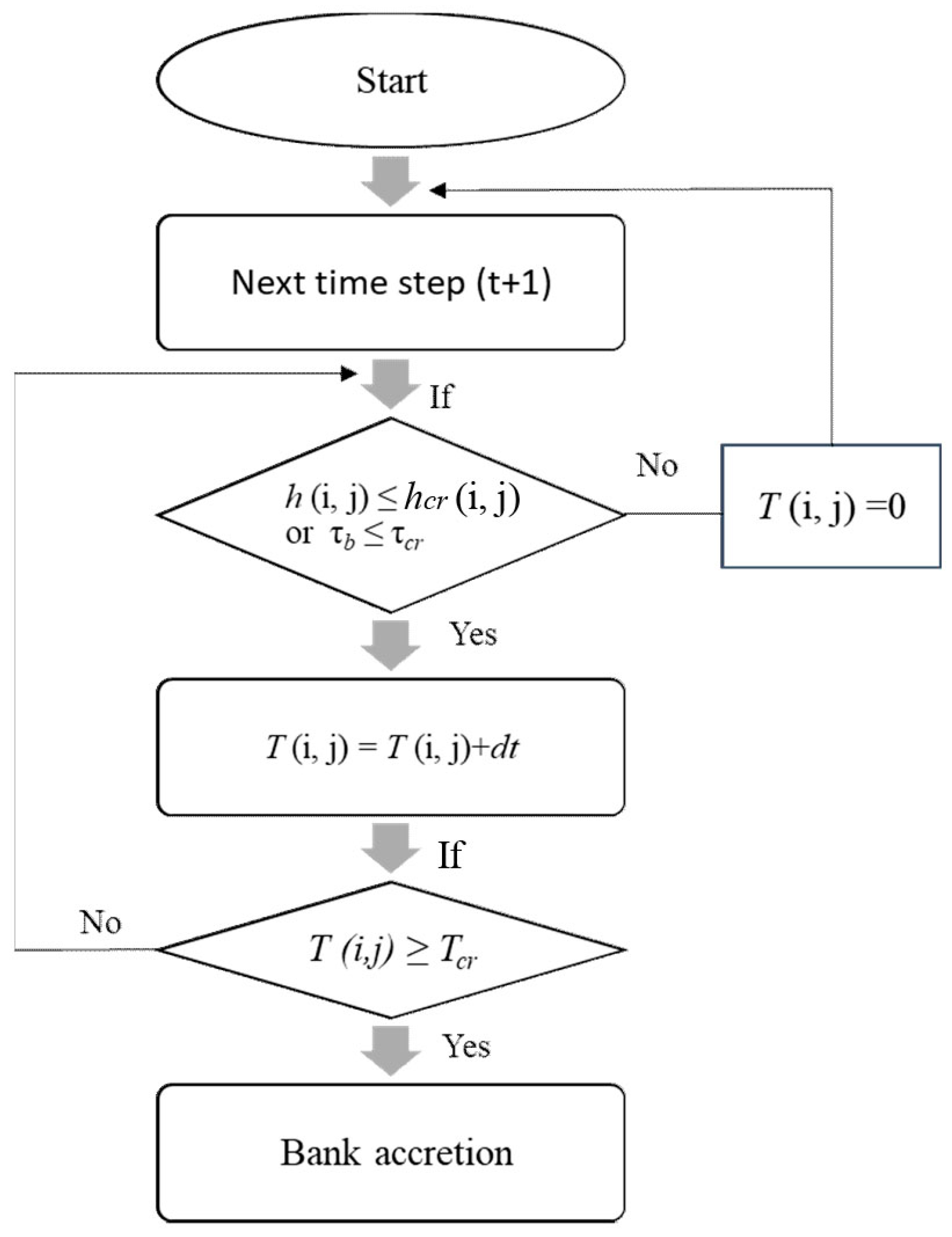
The channel width is determined as a result of the balance of bank accretion and bank erosion processes [1,2,6,10]. While bank erosion occurs in the outer part of a meander bend, bank accretion occurs mainly in the inner part [1]. For this reason, it was necessary to implement a model of bank accretion along the cross section. The bank accretion model is similar to the one proposed by Asahi et al. [10], considering a time for bank accretion, critical shear stress and water depth thresholds. The procedure for analysing the bank accretion is shown in Figure 1.
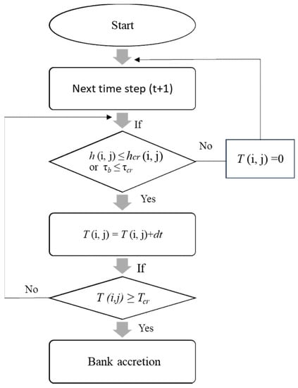
Figure 1.
Flow diagram for the bank accretion calculations where h is the water depth; hcr is the critical depth for landing; dt is the time step in the calculation; and T(i, j) is the sum of the time of consecutive steps over which h ≤ hcr or τb ≤ τbc, the accretion will occur in those cells where the time T (i, j) exceeds a critical time for occurrence of bank accretion Tcr(i, j).
For every time step, the programme checks if the water level becomes a value equal or smaller than a critical water depth hcr (minimum depth where accretion will occur), or else, the shear stress exerted by the flow is less than the critical shear stress of the bank. If one of these conditions is met for a time longer than the critical time Tcr, then the bank will recover its initial height.
In this paper, the values of critical depth hcr and the critical time Tcr were tuned in order to maintain, as much as possible, an averaged constant width. According to Asahi et al. [10], these values are highly dependent on the type of vegetation, hydrologic and climate regime, the deposited sediment among others and should be calibrated adequately.
2.5.2. Secondary Flow
The secondary flow of the first kind was included in Equation (15) as follows:
where ubs and ubn are the near-bed velocities in streamwise and transverse directions and N* is the coefficient of the strength of secondary flow (assumed to be 7.0 for simplicity, as proposed by Engelund [30]).
2.5.3. Centreline Migration
The meander migration was calculated as follows. First the width of the channel in each section was calculated at every time step and then the coordinates of the left and right banks were obtained. The left and right banks correspond to the point where the water intersects with the bank. The coordinate of the centre of the channel was calculated as:
where nL and nR are the left and right bank local coordinates; and ncnew is the coordinate of the central part of the channel.
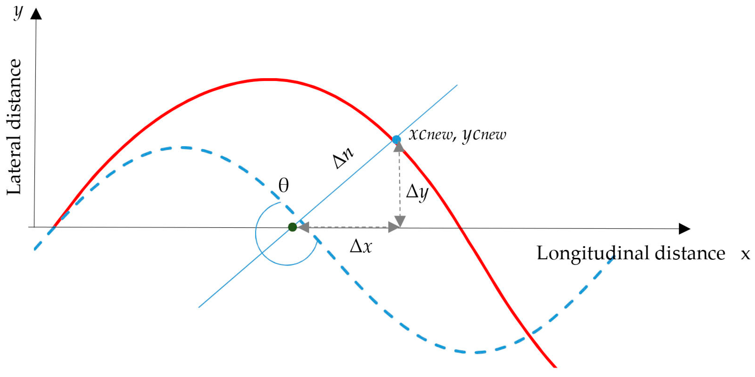
Then, the shifted distance Δn from the current centre of the channel to the previous one along the cross section (Figure 2) was calculated as follows.
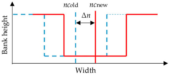
Figure 2.
Cross centreline migration (Blue: old cross section, red: New cross section).
The inclination θ of each cross-section with respect to x axis was considered. The coordinates of the new channel centreline were calculated as (Figure 3):
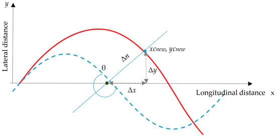
Figure 3.
Schematic representation of the centreline migration in plain view (blue: previous centreline, red: new centreline).
2.5.4. Parametric Cubic Splines (PCS)
The methodology explained previously for computing the channel centreline in each section will cause oscillations in the calculations. In order to obtain a smooth transition between sections, Parametric Cubic Splines (PCS) should be implemented [19]. The method applied in this paper is the same as suggested by Ichida et al. [31] for planar ordered scattered two-dimensional (2D) data.
The methodology consists of dividing the dataset into two equal parts. For each data set, PCS are calculated. Then, the programme judges if the smoothing at each section is adequate by using a Trend criterion. If the fitting it is adequate, then that will be the final curve but if not, the data is again divided in two parts and the process is repeated until an adequate fitting is obtained. This methodology improves the fitting by using a finite number of splines and guaranteeing a smooth transition between curves up to the first order derivative [31].
2.6. Model Comparison: RVR Meander and CP Model
The RVR meander migration model is the result of the coupling between the hydrodynamic model of Garcia et al. [11] (described in Section 2.1) with the bank erosion model CONCEPTS (Conservational Channel Evolution Pollutant Transport System) of Langendoen et al. [32]. This meander migration model developed by Motta et al. [18] is able to reproduce more rich variety of planform shapes such as high skewness and sharp necks compared to the classic approach of Ikeda et al. [21]. In addition, the model can simulate the development of downstream skewed meander bends, compound loops, and rectangular shapes [18]. However, as pointed out by the authors of [18,33], the model was limited by: (1) the lack of connection between hydrodynamics and sediment dynamics which means that bed forms such as bars cannot be represented by the model; (2) uniform bed material; (3) constant channel width which means that the model does not provide a physically-based description of the bank accretion processes; and (4) eroded bank soils are transported as suspended load out of the modelling reach.
Regarding the bank erosion, the RVR model considered planar and cantilever failures using a limit equilibrium method. Among the different types of cantilever failures, the model reproduces shear type failures. In contrast, the CP model is able to represent cantilever failures of the shear and beam type. This is important because beam failure is considered to be the dominant failure mechanism in cantilever failures [20,34].
If bank failure occurs, the RVR model calculates the volume of failed material and converts it to lateral flux of sediment into the channel [35]. The slump blocks protection is considered similarly as in Parker et al. [2] using a reduction factor Karmor which is a function of the volume of slump blocks [1]. This reduction factor is calculated as:
where Ablock,total is the volume per unit streamwise distance of the slump blocks generated by cantilever and planar failure processes and c is a coefficient that amplifies the effect of slump block bank protection if greater than 1.0 and dampens the effect if lower than 1.0. Similarly, Patsinghasanee et al. [20] considered the Ksb factor (Equation (13)) to take into account the effect of the slump blocks. If Ksb is greater than 1.0 the erosion rate of slump blocks is increased and decreases if the value is less than 1.0.
The RVR model did not consider the block size and location of failed material at the toe of the bank but instead they consider a factor c to indirectly represent these effects. In contrast, the CP model assumes that the size and position of the slump blocks in the riverbed depends on the type of failure (shear type or beam type failure) as it was explained in Section 2.2.
The slump block decay process in the RVR model is considered using the methodology of Parker et al. [2] which consists of selecting a characteristic period of existence for slump blocks Tblock which is calculated as follows:
where Ablock,total,initial is the volume of slump blocks after the last flood, and Tblock is a characteristic period of existence for slump blocks representing the dynamics of slump block decay.
The CP model describes directly the reduction of the block size by considering fluvial erosion of the slump blocks (Equation (13)) and therefore the time of slump blocks decay depends on the size of slump blocks, erosion rate of slump blocks and the previous slump blocks volume that remains in the banks. In addition, bank accretion may occur if the conditions are adequate (see Section 2.5.1) and therefore erosion rates may be reduced.
One advantage of the RVR model is that it considers the vertical and horizontal heterogeneity of the soil distribution. The model is capable of modelling the different layers of materials in banks. This feature is not considered by the CP model. Instead, the CP model assumes the bank material to be a homogenous mixture of sand with silt and clay.
3. Numerical Experiments with the Model
The model was tested in eight cases. The first cases (Cases 1 to Case 6) correspond to a small scale (experimental scale) sine-generated curved channel. The bank material and hydraulics data is set similar to values used in the experiments of Patsinghasanee et al. [20]. In cases 7 and 8, the model was compared to results of the simulations of Motta et al. [18].
3.1. Case: Small Scale Sine-Generated Channel
The main objective of the numerical experiments is to determine the effect of the curvature, slump blocks and bank accretion in the cross sections. A cross section in the straight part of the channel is compared with a section in the sinusoidal part. The formation of cut-offs is not considered in the model. Therefore, the results showed here corresponds to the meander development before cut-offs occurrence. In addition, simulations were performed to investigate the effect of the bank strength in the development of the plan shape of the meander, varying the values of critical shear stress and maintaining all the other variables constant.
Initial Conditions
The geometry of the cross section and the hydraulic conditions are similar to the ones used in the experiments of Patsinghasanee et al. [20]. A rectangular channel with a height of 0.2 m and a channel width of 0.3 m was considered (Figure 4). Other conditions for the numerical simulations are listed in Table 1.
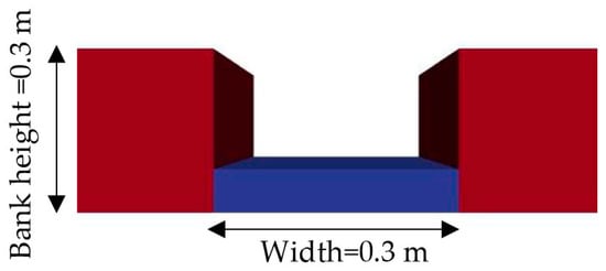
Figure 4.
Initial cross section for the simulations.

Table 1.
Numerical conditions for the simulations.
The initial plan shape consists of a straight channel of 4 m, one sinuous section of 8 m and again a straight channel with a length of 16 m (Figure 5). The total length equals to 28 m. The sinuous part of the channel is generated by the sine-generated curve equation:
where is the initial angle of the sine-generated curve, L is the length of the channel centreline over one meander cycle and s is coordinate along the curve. The initial meander angle θ0 was set equal to 20°. The channel in total is composed of 71 nodes, where Section 21 (S-21) is located in the apex of the bend and Section 50 (S-50) is located in the straight part of the channel, as shown in Figure 5.

Figure 5.
Top view of the initial channel centreline.
The six simulated cases are shown in Table 2. Case 1 includes the effect of slump blocks and bank accretion. In Case 2, slump blocks were neglected. In Case 3, bank accretion was not considered. Cases 4 to 6 were variations of Case 1 and employed different values of critical shear stress that varied from 0.073 Pa to 0.61 Pa (calculated using Equations (11) and (12), respectively).

Table 2.
Simulated cases for small scale.
3.2. Results
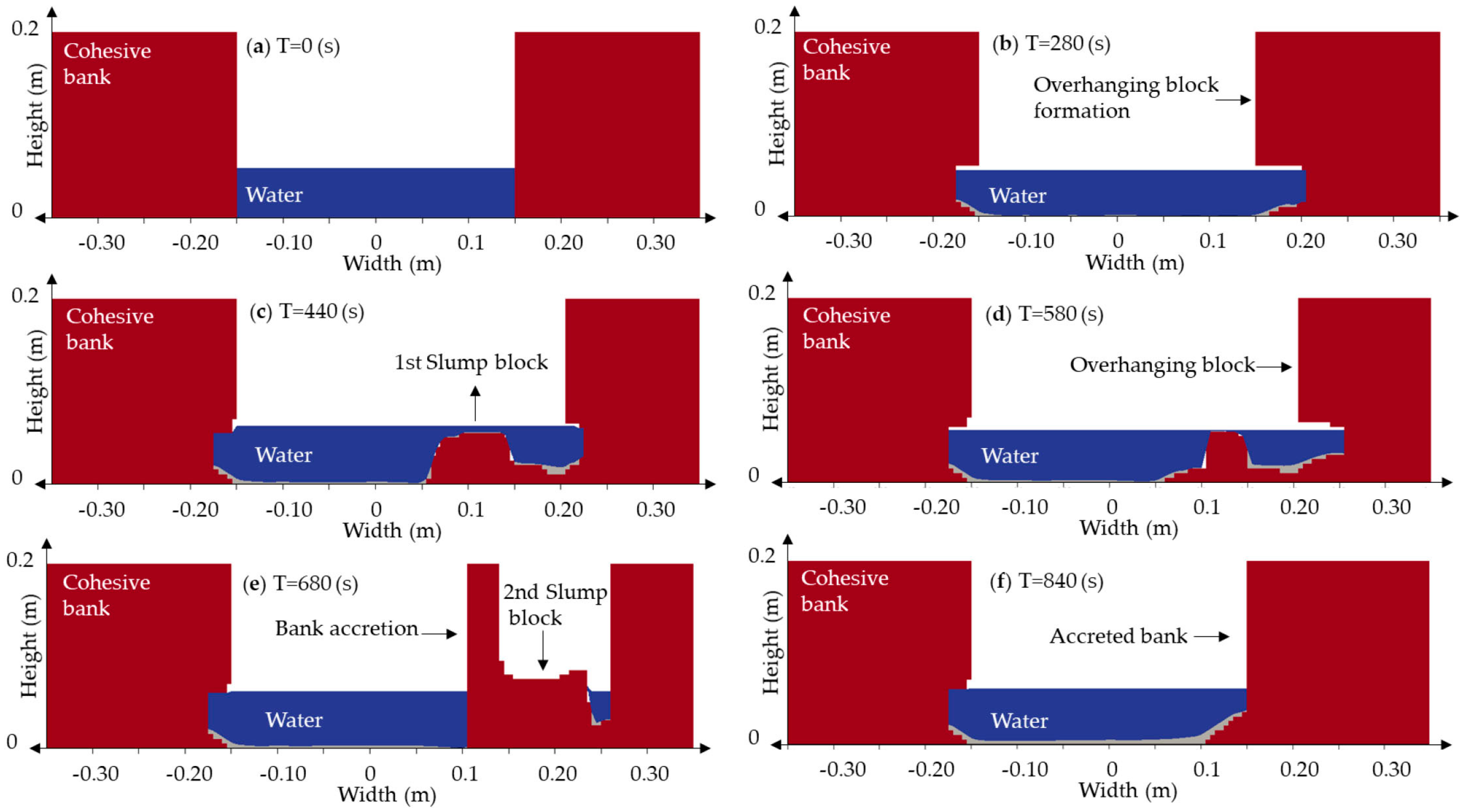
Figure 6 shows the cross sectional results of the different processes observed in the numerical simulations. The initial rectangular shape (Figure 6a) is shown at T = 0 (s). Then, fluvial erosion in the lower part of the channel in both banks occurs where overhanging blocks are observed in both banks (Figure 6b). However, the fluvial erosion rate is faster in the outer bank (T = 280 s). At T = 440 s (Figure 6c), the overhanging block in the outer banks has collapsed and then, the decomposition process of the slump block starts. After 580 (s), the slump block has been reduced and the bank is eroded again (Figure 6d). At this point, the water level has decreased due to widening of the section and, the upper part of the slump block fits the condition for bank accretion. At 680 s (Figure 6e), bank accretion and bank erosion occurred at the same time. Also, a second failure of the bank is observed. Finally, after 840 (s), bank accretion occurred in upper part of the slump block (Figure 6f).

Figure 6.
Sequence of bank erosion and bank accretion processes for Case 1: (a) Initial section; (b) fluvial erosion in the lower part of the bank and overhanging block failure; (c) Slump block decomposition; (d) widening of the channel; (e) accretion starts and (f) recovering of the initial bank height (Right: outer bank, left: inner bank).
3.2.1. Slump Blocks Effect
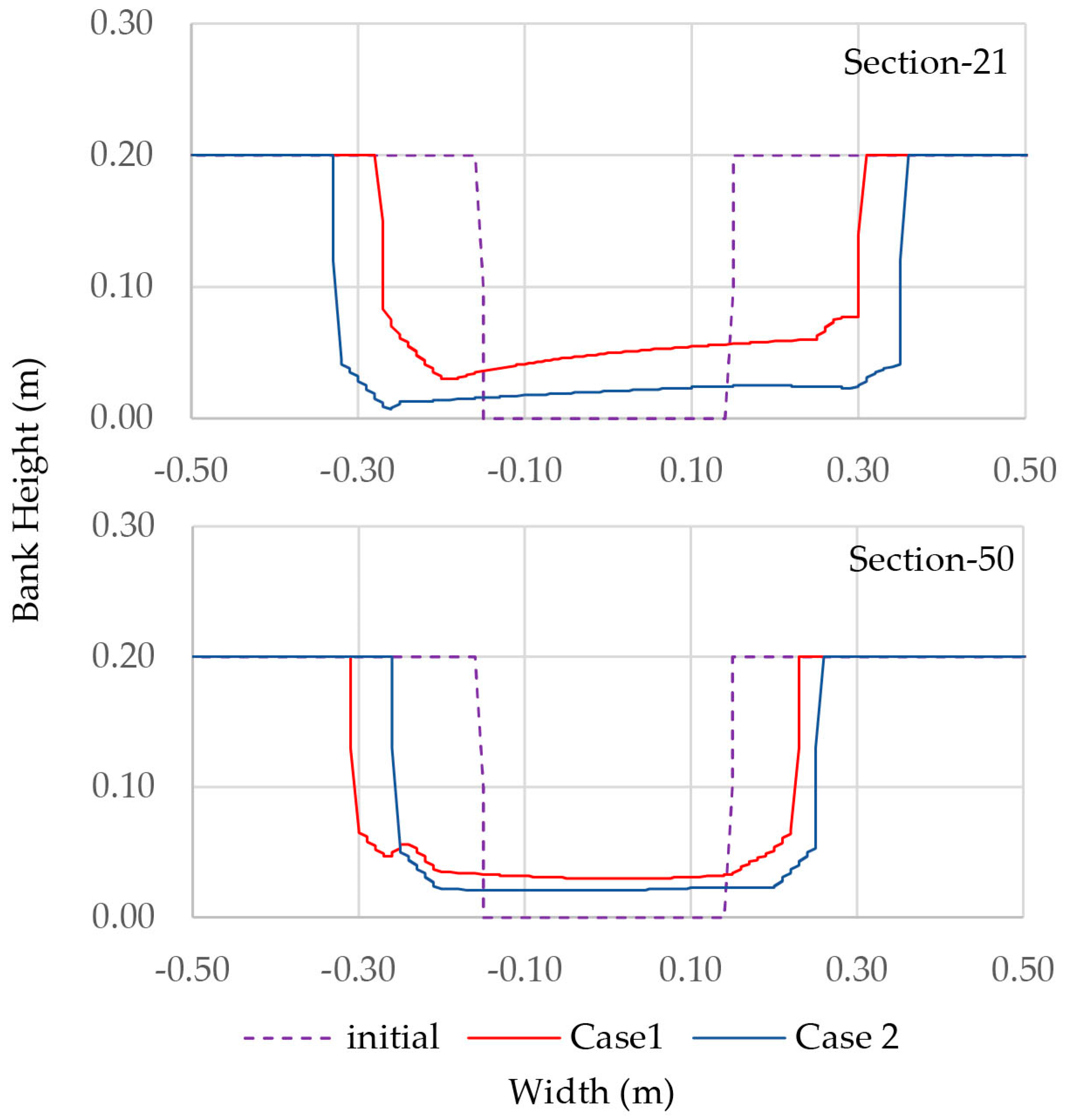
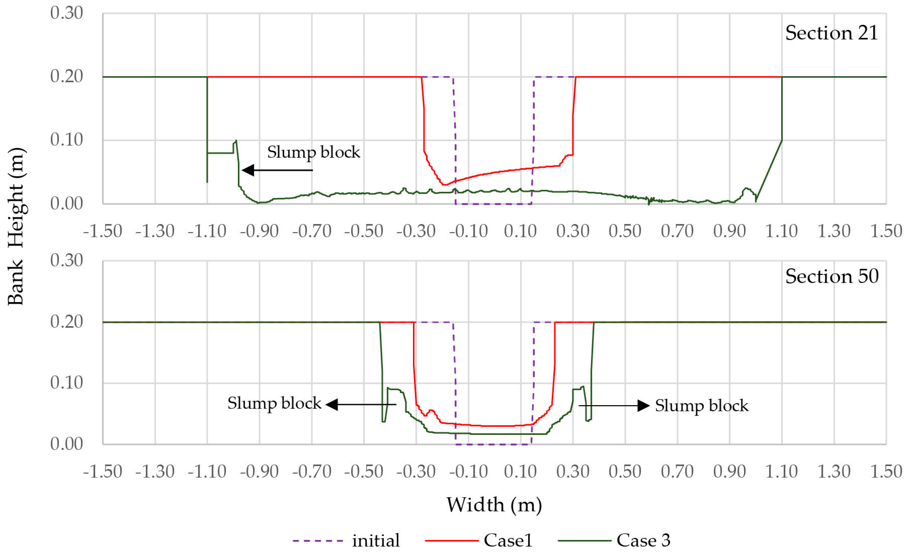
The cross-sectional results after six hours of simulation are plotted in Figure 7.
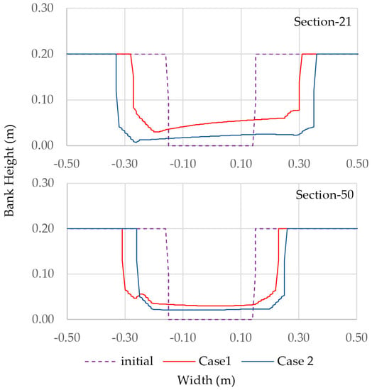
Figure 7.
Comparison of cross sectional evolution for cases 1 and 2 in the straight part of the channel (S-50) and the curved part of the channel (S-21) for a simulation time of 21,600 (s).
In the curved (S-21) and straight (S-50) parts of the channel, the erosion rate was higher when slump blocks were neglected. The cross section in the straight part (S-50) keeps a squared shape in both cases (Cases 1 and 2) while in the curved part (S-21), a lateral inclination in the bed slope profile was observed. Figure 8a shows the variation of the channel width for Case 1. At the end of the simulations, the channel width has increased almost twice its initial length in the straight (0.46 m) and curved parts (0.54 m). However, the width variation is more obvious in the curved part of the channel where abrupt reduction of the channel width is observed due to slump blocks failures and bank accretion. Figure 8b illustrates the increasing tendency in the channel width for Case 2 where slumps blocks are neglected. In the curved part (S-21) the channel width is equal to 0.69 m while in the straight part (S-50) the width is around 0.52 m.
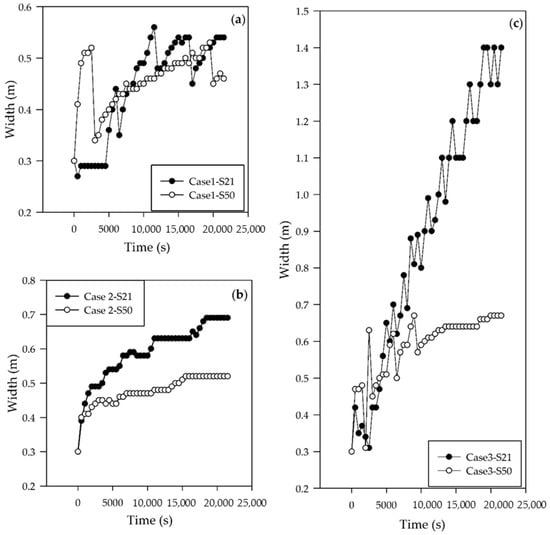
Figure 8.
Width variation for (a) Cases 1, (b) 2 and (c) 3 in the straight (S-50) and curved part (S-50) of the channel.
3.2.2. Bank Accretion Effect
Bank accretion effect was more evident in the curved part of the channel (S-21). Figure 9 illustrates the cross-sectional comparison between Cases 1 and 3. The channel width increased around five times the original width (1.4 m) when bank accretion was not considered (Case 3) as it is shown in Figure 8c. In addition, same mechanism was observed in the straight part of the channel (S-50) but the magnitude was smaller (0.66 m). The bank accretion process in this paper is taken into account by a simple threshold of water level depth, critical shear stress and time (see Section 2.5.1). These parameters take into account the effect of different variables such as vegetation encroachment and the difference between time scales in the bank erosion and bank accretion processes. The effect of the bank accretion model is to keep a balance between bank erosion rates and bank accretion rates, therefore it controls the widening in the cross section.
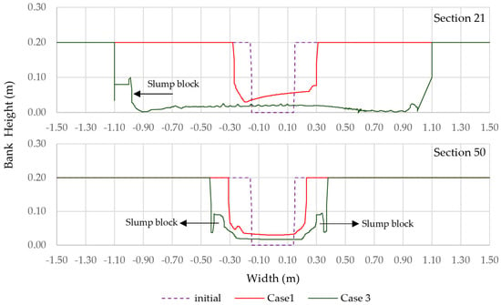
Figure 9.
Comparison of cross sectional evolution for cases 1 and 3 in the straight part of the channel (S-50) and the curved part of the channel (S-21) for a simulation time of 21,600 (s).
3.2.3. Effect of Bank Strength in the Plan Shape
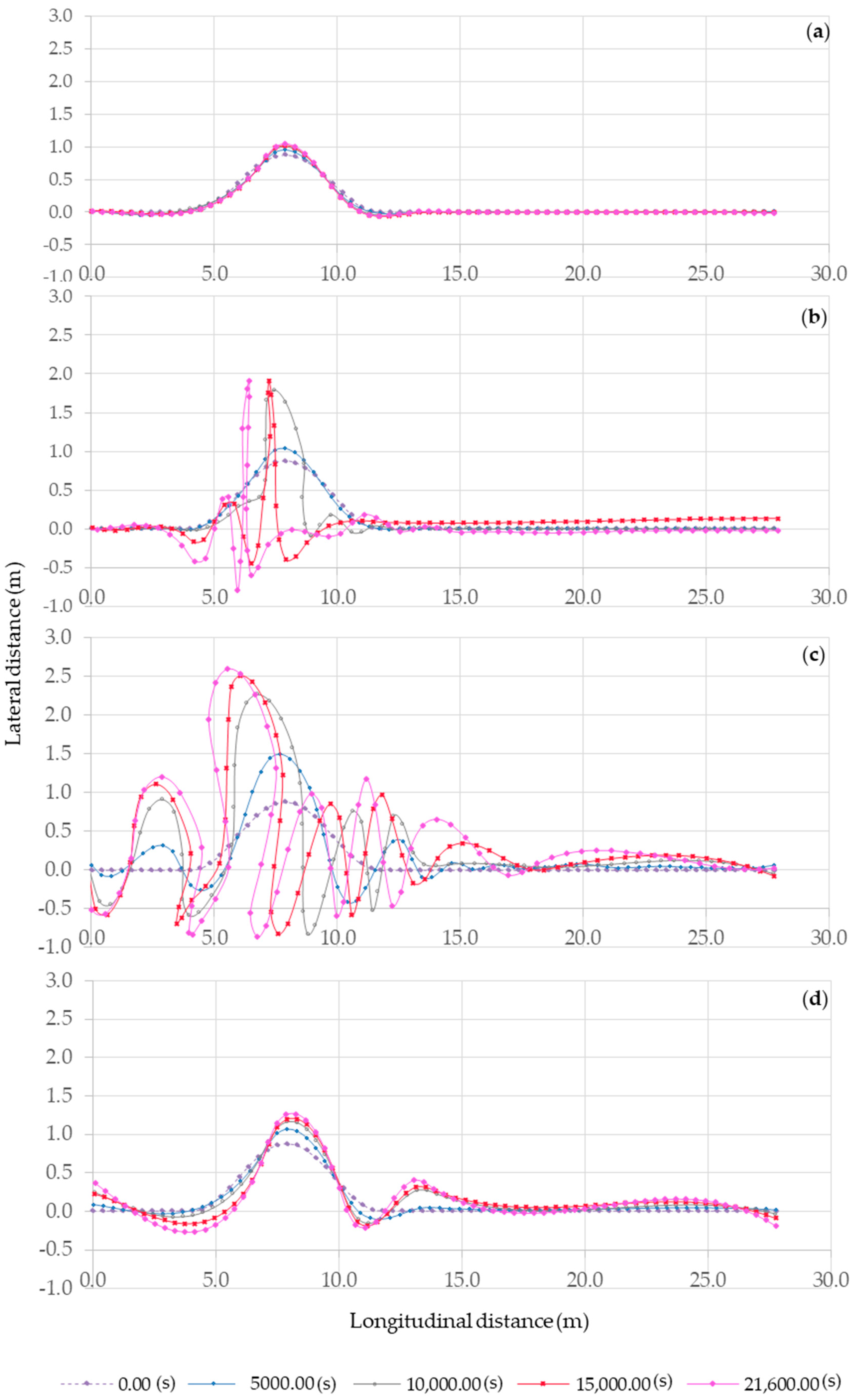
The planform shapes obtained in each case were plotted at different times from 0 to 21,600 s. As shown in Figure 10a, in Case 1, the plan shape remains similar to the initial channel planform with small changes in the points where the curvature changes. When the critical shear stress was equal to 0.2 Pa (Figure 10b), the calculations became unstable and the meander wavelength was reduced. Lateral expansion and development of small meanders were observed for a critical shear stress of 0.4 Pa (Figure 10c). The highest value of critical shear stress (0.61 Pa) showed less lateral migration than the previous case (Figure 10d).
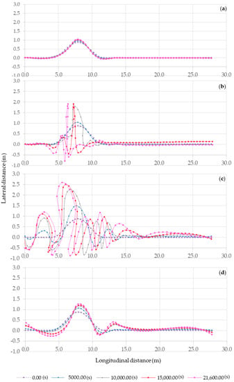
Figure 10.
Meander migration of the channel centreline from time = 0 to Time = 21,600 s for different values of critical shear stresses where: (a) τc = 0.073 Pa, (b) τc = 0.2Pa, (c) 0.40 Pa, and (d) 0.61 Pa.
3.3. Case: Large Scale Sine-Generated Curve
3.3.1. Initial Conditions
The CP model is applied to the meandering case “d” of Motta et al. [18] in order to compare both models. The initial channel shape corresponds to a sine-generated alignment with arc-wavelength of 1000 m and crossover angle of 70°. The length of the initial channel is 7494 m. The hydraulics conditions for the simulations are shown in Table 3.

Table 3.
Numerical values used for large scale case (Motta et al.’s case).
As explained in Section 2.6, the model of Motta et al. [18] considers, the effect of the vertical heterogeneity of the soil. The bank is assumed to be composed of different layers of materials. The upper layers is a less erodible material compared with the lower layer and each layer considered different values for the erodibility coefficient. More detailed information of the numerical values used in the simulations can be found in Motta et al. [18]. However, the CP model consider the bank as a homogenous mixture of sand and silt and therefore it is necessary to select a unique value of erodibility coefficient. Given the general lack of data to perform the simulations different values for erodibility coefficient and critical shear stress were tested. The following values were selected for the simulations: erodibility coefficient kd was varied from 1000 m3/Ns (Case 7) to 5000 m3/Ns (Case 8) with a critical shear stress of 0.2 Pa.
3.3.2. Results
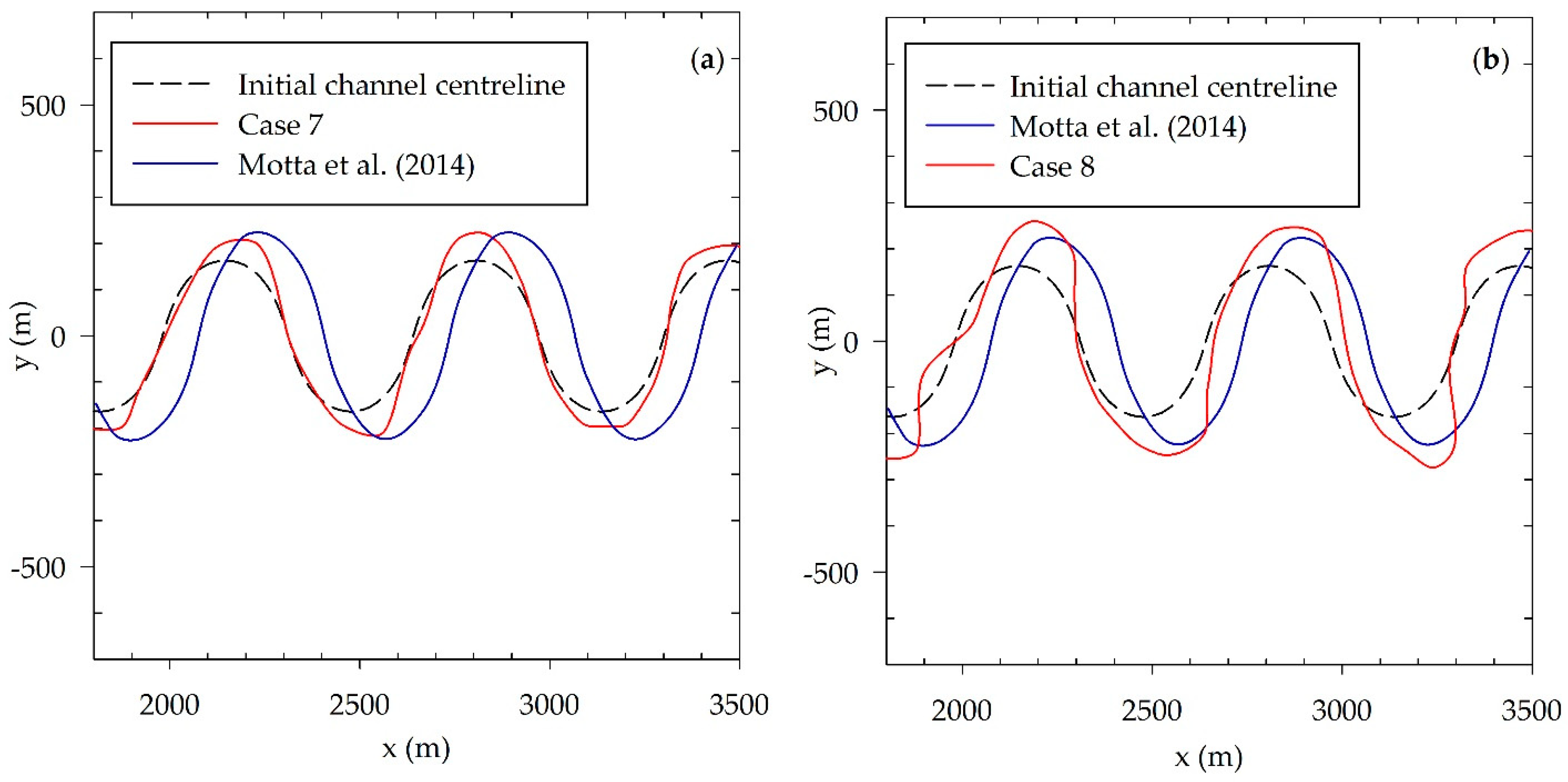
Figure 11 compares simulated migration centrelines between the results of Motta et al. [18] after 4 years of simulations with the CP model (Case 7 and Case 8).
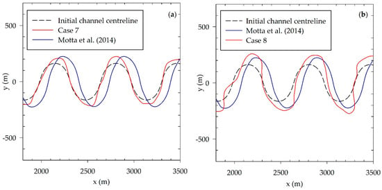
Figure 11.
Comparison of Cases 7 and 8 with the simulations of Motta et al. [18]: (a) Case 7 and (b) Case 8.
The simulation time for each case was different. Figure 11a shows the results of the simulations after 0.33 years for Case 7 and Figure 11b for Case 8 after 0.63 years of simulations. When comparing the results of Case 7 with the results of Motta et al. [18], it can observed that the amplitude of the wavelength is similar in both cases. However, the lateral migration in the downstream was larger in the case of Motta et al. [18]. In Case 8, similar situation was observed but lateral migration rates were higher in Case 8. The shape of the meander was also changed. While in the case of Motta et al. the bends seems symmetrical and skewed upstream, Cases 7 and 8 showed asymmetrical shapes. In Case 7 the upstream bend points downstream while the downstream bend points upstream. In Case 8, the bends were skewed downstream, compared with Motta et al.’s case.
4. Discussion
The correction of the velocity profile by a near bank velocity, which is dependent on the curvature variation, was observed in each cross section. As expected, the curvature effect was higher in the apex of the bend. However, the effect of the Parametric Cubic Splines (PCS) on the curvature controlled the excessive change in the curvature between sections especially when there was sudden change in the curvature (i.e., connection point between the straight and curved part).
When we compared the section in the straight part of the channel with the one in the apex of the meander, the erosion was larger towards the outer bank. Larger erosion rates increased the number of slump blocks and slump blocks stopped erosion of the bank until the block was decomposed. However, slump blocks promoted accretion when the blocks were big enough and not submerged. This relation between slump blocks and bank accretion kept a relatively constant width. Even though bank accretion was represented in a very conceptual manner, it was clear that it played an important role in regulating the width of the cross section.
The planform shape was regulated by the curvature and the bank strength was represented by the critical shear stress. The bank strength, bank accretion and erosion rates determined the channel shape. As the values of the critical shear stress values increased, the channel reached a constant width.
The CP model is limited by the fact that several parameters are needed to be determined experimentally or locally in order to validate this model. Two parameters that are very important in this model are the erodibility coefficient for slump blocks erosion ksb and the critical time considered for bank accretion to occur Tcr. In this paper, we consider that the slump blocks decompose at a rate 20% faster than the original banks [7]. The critical water depth value in which land accretion occurs (hcr) and the critical time Tcr were adjusted in order to obtain an average constant width. Nevertheless, as slump blocks depend on erosion rates and the bank accretion depends on slump blocks as well, the width varied in each section and in time.
Another limitation of the model is that neglects the occurrence of cut-offs. This was particularly clear for Case 4, where the plan shape of the channel at the bend changed in such a way that cut-offs were really close to occurring (Figure 10b).
The comparison of the CP model with the results of Motta et al. [18] presented some differences between both results in terms of the lateral migration, the migration time and the shape of the bends. These difference in the results can be explained by the bank erosion model considered in each model. As it was explained before, Motta et al. [18] model considered a two layer model for their simulations while the presented model considers the bank as a homogenous mixture of sand with silt-clay. The second reason is the difference between the parameters used in each model. For example, the value of Ksb in the present model is constant and is determined by tuning the value with experimental values of width. In the model of Motta et al. [18] they considered the factor Karmor, which is dependent on the slump blocks volume and the residence time of slump blocks Tblock. The residence time in our model is determined by the erosion rate of the slump blocks and the size of the slump blocks which also depends on the type of cantilever failure (Shear or beam type). However, the results suggest that the CP model is capable of simulating asymmetrical bends.
5. Conclusions
The improved numerical model presented in this study was used to study cantilever failures with slump blocks in a curved channel. The methodology proposed here allows us to study the changes in the cross-sections due to the variation in the streamwise curvature. Furthermore, by including a bank accretion model we attempted to show the evolution in the planform shape of the channel.
The model showed to be highly sensitive to the change of the values of critical shear stresses. Depending on the value of the critical shear stress, the plan shape of the channel changed, developing wavy features in the downstream direction. Nevertheless, it should be considered that the critical shear stress controls the narrowing and the widening of the channel in this model. For higher values of critical shear stresses, the sections become narrower and for smaller values of critical shear stresses the section widens. The results also indicate that slump blocks increased the rate of bank accretion and therefore, reduce the channel width.
The experimental and large-scale simulations performed in this study indicates that the parameters need to be calibrated carefully for each case. The next step in order to simulate midterm and long plan shape evolution of meandering channels should be the consideration of cut-offs, as cut offs are an intrinsic characteristic of meanders.
Author Contributions
Investigation, K.R.A.F.; Supervision, S.P.; Writing—original draft, K.R.A.F.; Writing—review and editing, S.P., I.K. and Y.S.
Funding
This research received no external funding.
Acknowledgments
The authors would like to express their sincere gratitude to the Japanese Government Scholarships for financial support of scholarships.
Conflicts of Interest
The authors declare no conflict of interest.
References
- Crossato, A. Analysis and Modelling of River Meandering/Analyses en Modellering van Meanderende Rivieren; IOS Press: Amsterdam, The Netherlands, 2008. [Google Scholar]
- Parker, G.; Shimizu, Y.; Wilkerson, G.V.; Eke, E.C.; Abad, J.D.; Lauer, J.W.; Paola, C.; Dietrich, W.E.; Voller, V.R. A new framework for modeling the migration of meandering rivers. Earth Surf. Process. Landf. 2011, 36, 70–86. [Google Scholar] [CrossRef]
- Eke, E.C.; Czapiga, M.J.; Viparelli, E.; Shimizu, Y.; Imran, J.; Sun, T.; Parker, G. Coevolution of width and sinuosity in meandering rivers. J. Fluid Mech. 2014, 760, 127–174. [Google Scholar] [CrossRef]
- Kleinhans, M.G.; Schuurman, F.; Bakx, W.; Markies, H. Meandering channel dynamics in highly cohesive sediment on an intertidal mud flat in the Westerschelde estuary, The Netherlands. Geomorphology 2009, 105, 261–276. [Google Scholar] [CrossRef]
- Ferreira da Silva, A.M.; Ebrahimi, M. Meandering Morphodynamics: Insights from Laboratory and Numerical Experiments and Beyond. J. Hydraul. Eng. 2017, 143, 03117005. [Google Scholar] [CrossRef]
- Kleinhans, M.G.; van den Berg, J.H. River channel and bar patterns explained and predicted by an empirical and a physics-based method. Earth Surf. Process. Landf. 2011, 36, 721–738. [Google Scholar] [CrossRef]
- Eke, E.; Parker, G.; Shimizu, Y. Numerical modeling of erosional and depositional bank processes in migrating river bends with self-formed width: Morphodynamics of bar push and bank pul. J. Geophys. Res. Earth Surf. 2014, 119, 1455–1483. [Google Scholar] [CrossRef]
- Van de Lageweg, W.I.; van Dijk, W.M.; Baar, A.W.; Rutten, J.; Kleinhans, M.G. Bank pull or bar push: What drives scroll-bar formation in meandering rivers? Geology 2014, 42, 319–322. [Google Scholar] [CrossRef]
- Schuurman, F.; Shimizu, Y.; Iwasaki, T.; Kleinhans, M.G. Geomorphology Dynamic meandering in response to upstream perturbations and floodplain formation. Geomorphology 2016, 253, 94–109. [Google Scholar] [CrossRef]
- Asahi, K.; Shimizu, Y.; Nelson, J.; Parker, G. Numerical simulation of river meandering with self-evolving banks. J. Geophys. Res. Earth Surf. 2013, 118, 2208–2229. [Google Scholar] [CrossRef]
- Garcia, M.H.; Bittner, L.; Nino, Y. Mathematical Modeling of Meandering Streams in Illinois: A Tool for Stream Management and Engineering; University of Illinois at Urbana-Champaign: Urbana, IL, USA, 1996; pp. 1–63. [Google Scholar]
- Hackney, C.; Best, J.; Leyland, J.; Darby, S.E.; Parsons, D.; Aalto, R.; Nicholas, A. Modulation of outer bank erosion by slump blocks: Disentangling the protective and destructive role of failed material on the three-dimensional flow estructure. Geophys. Res. Lett. 2015, 42, 10–663. [Google Scholar] [CrossRef]
- Mosselman, E. A review of mathematical models of river planform changes. Earth Surf. Process. Landf. 1995, 20, 661–670. [Google Scholar] [CrossRef]
- Langendoen, E.J.; Mendoza, A.; Abad, J.D.; Tassi, P.; Wang, D.; Ata, R.; El kadi Abderrezzak, K.; Hervouet, J.M. Improved numerical modeling of morphodynamics of rivers with steep banks. Adv. Water Resour. 2016, 93, 4–14. [Google Scholar] [CrossRef]
- Patsinghasanee, S.; Kimura, I.; Shimizu, Y.; Nabi, M.; Chub-Uppakarn, T. Coupled studies of fluvial erosion and cantilever failure for cohesive riverbanks: Case studies in the experimental flumes and U-Tapao River. J. Hydro-Environ. Res. 2017, 16, 13–26. [Google Scholar] [CrossRef]
- Patsinghasanee, S.; Kimura, I.; Shimizu, Y.; Todate, T. Experimental Investigations on Cantilever Failures for Cohesive Riverbanks. J. Jpn. Soc. Civ. Eng. 2016, 72, 769–774. [Google Scholar] [CrossRef]
- Samadi, A.; Davoudi, M.H.; Amiri-Tokaldany, E. Experimental Study of Cantilever Failure in the Upper Part of Cohesive Riverbanks. Res. J. Environ. Sci. 2011, 5, 444–460. [Google Scholar] [CrossRef]
- Motta, D.; Langendoen, E.J.; Abad, J.D.; Garcia, M.H. Modification of meander migration by bank failures. J. Geophys. Res. Earth Surf. 2014, 119, 1026–1042. [Google Scholar] [CrossRef]
- Motta, D. Meander Migration with Physically-Based Bank Erosion. Ph.D. Thesis, University of Illinois at Urbana-Champaing, Urbana, IL, USA, 2013. [Google Scholar]
- Patsinghasanee, S.; Kimura, I.; Shimizu, Y. Numerical Simulation of a Cantilever Failure with the Effect of Slump Blocks for Cohesive Riverbanks. J. Jpn. Soc. Civ. Eng. 2016, 72, 493–498. [Google Scholar] [CrossRef]
- Ikeda, S.; Parker, G.; Sawai, K. Bend theory of river meanders-1. Linear development. J. Fluid Mech. 1981, 112, 363–377. [Google Scholar] [CrossRef]
- Partheniades, E. Erosion and deposition of cohesive soils. J. Hydraul. Div. 1965, 91, 105–139. [Google Scholar]
- Julian, J.P.; Torres, R. Hydraulic erosion of cohesive riverbanks. Geomorphology 2006, 76, 193–206. [Google Scholar] [CrossRef]
- Smerdon, E.; Beasley, R. Critical tractive forces in cohesive soils. Agric. Eng. 1961, 42, 26–29. [Google Scholar]
- Arnez Ferrel, K.R.; Kimura, I.; Shimizu, Y. Numerical modeling of bank erosion in a circular channel with cohesive banks including effect of slump blocks. J. Japan Soc. Civ. Eng. 2017, 73, 579–586. [Google Scholar]
- Patsinghasanee, S.; Kimura, I.; Shimizu, Y.; Nabi, M. Experiments and modelling of cantilever failures for cohesive riverbanks. J. Hydraul. Res. 2018, 56, 76–95. [Google Scholar] [CrossRef]
- Ashida, K.; Michiue, M. Michiue Study on hydraulic resistance and bed load transport rate in alluvial streams. Proc. Jpn. Soc. Civ. Eng. 1972, 206, 59–69. [Google Scholar] [CrossRef]
- Iwagaki, Y. Hydrodynamical study on critical tractive force. Trans. JSCE 1956, 41, 1–21. [Google Scholar] [CrossRef]
- Hasegawa, K. Hydraulic Research on Planimetric Forms, bed topographies and flow in alluvial River. Ph.D. Thesis, Hokkaido University, Hokkaido, Japan, 1984. [Google Scholar]
- Engenlung, F. Flow and bed topography in channel bends. J. Hydraul. Div. 1974, 100, 1631–1648. [Google Scholar]
- Ichida, K.; Kiyono, T.; Yoshimoto, F. Curve fitting by a one pass method with a piecewise cubic polynomial. ACM Trans. Math. Softw. (TOMS) 1977, 3, 164–174. [Google Scholar] [CrossRef]
- Langendoen, E.J.; Alonso, C.V. Modeling the Evolution of Incised Streams: I. Model Formulation and Validation of Flow and Streambed Evolution Components. J. Hydraul. Eng. 2008, 134, 749–762. [Google Scholar] [CrossRef]
- Motta, D.; Abad, J.D.; Langendoen, E.J.; Garcia, M.H. A simplified 2D model for meander migration with physically-based bank evolution. Geomorphology 2012, 163–164, 10–25. [Google Scholar] [CrossRef]
- Patsinghasanee, S.; Kimura, I.; Shimizu, Y.; Nabi, M. Cantilever failure investigations for cohesive riverbanks. Proc. Inst. Civ. Eng. Water Manag. 2017, 170, 93–108. [Google Scholar] [CrossRef]
- Langendoen, E.J. CONCEPTS—Conservational Channel Evolution and Pollutant Transport System; USDA-ARS National Sedimentation Laboratory: Oxford, UK, 2000; p. 160.
© 2018 by the authors. Licensee MDPI, Basel, Switzerland. This article is an open access article distributed under the terms and conditions of the Creative Commons Attribution (CC BY) license (http://creativecommons.org/licenses/by/4.0/).

