Abstract
Geometric heights, defined with respect to a geometric reference surface, are the most commonly used in planetary studies, but the use of physical heights defined with respect to an equipotential surface (typically the geoid) has been also acknowledged for specific studies (such as gravity-driven mass movements). In terrestrial studies, the geoid is defined as an equipotential surface that best fits the mean sea surface and extends under continents. Since gravimetric geoid modelling under continents is limited by the knowledge of a topographic density distribution, alternative concepts have been proposed. Molodensky introduced the quasigeoid as a height reference surface that could be determined from observed gravity without adopting any hypothesis about the topographic density. This concept is widely used in geodetic applications because differences between the geoid and the quasigeoid are mostly up to a few centimeters, except for mountainous regions. Here we discuss the possible applicability of Molodensky’s concept in planetary studies. The motivation behind this is rationalized by two factors. Firstly, knowledge of the crustal densities of planetary bodies is insufficient. Secondly, large parts of planetary surfaces have negative heights, implying that density information is not required. Taking into consideration the various theoretical and practical aspects discussed in this article, we believe that the choice between the geoid and the quasigeoid is not strictly limited because both options have advantages and disadvantages. We also demonstrate differences between the geoid and the quasigeoid on Mercury, Venus, Mars and Moon, showing that they are larger than on Earth.
1. Introduction
Physical heights on Earth are reckoned with respect to the geoid, which is defined by Gauss [1] as an equipotential surface that best fits (in a least-squares sense) the global mean sea surface. Under continents, the geoid could be determined from gravity according to Stokes’ [2] theory, but observed gravity data have to be corrected for the gravitational contribution of topographic masses. This procedure requires knowledge of the topographic density distribution. Ascertaining that the topographic density could not be determined accurately, Molodensky [3] introduced the concept of the quasigeoid surface, which serves as a practical height reference surface to define the normal heights without adopting any hypothesis about the topographical density distribution. The differences between the geoid and the quasigeoid (i.e., the geoid-to-quasigeoid separation) were found to be typically within a few centimeters, with maxima in mountainous regions reaching a few meters [4,5,6,7], while completely negligible offshore [8].
In planetary studies, geometric heights are widely used instead of physical heights. Nevertheless, studies of gravity-driven mass movements (lava, ice, and aquifers), deep mantle density heterogeneities, lithospheric stresses and other geophysical and geodynamic phenomena can be studied and interpreted based on an accurately known equipotential geometry, or equivalently physical heights referred to an equipotential surface. The definition of physical heights for planetary bodies, however, differs from terrestrial applications due to the absence of liquid oceans. The choice of the equipotential surface is then usually closely referenced with respect to a mean reference spheroid or ellipsoid, which best fits the topographic shape of a particular planetary body; more discussion about this issue can be found in Reference [9]. In this case, large parts of planetary surface have negative heights, while only fractions of the continental land surface on Earth are below sea level. This brings the question of possible use of Molodensky’s concept in planetary studies because, in the case of negative physical heights, information about topographic density is naturally not required. Moreover, the crustal density of planetary bodies is much less known than Earth’s upper crustal density, thus affirming even more the major argument of Molodensky about introducing the concept of normal heights and the quasigeoid. The situation of defining physical heights on Earth and planetary bodies is schematically illustrated in Figure 1.
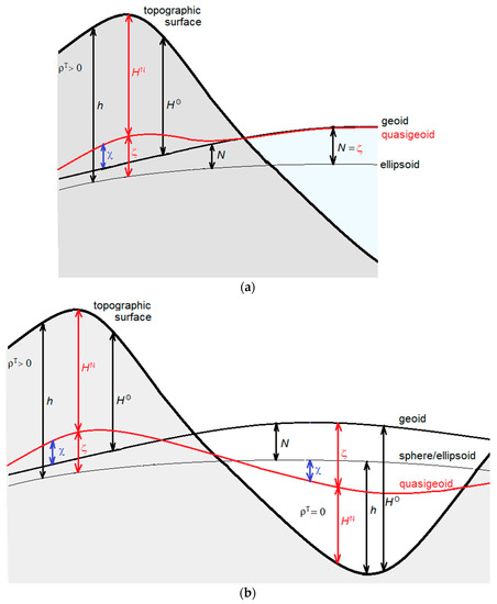
Figure 1.
Definition of physical heights on (a) Earth and (b) planetary bodies. Notation: the geometric height, the orthometric height, the normal height, the geoid height, the quasigeoid height, and the geoid-to-quasigeoid separation.
In this study, we address these theoretical and practical aspects and investigate the possibility of using Molodensky’s concept in planetary studies. In addition, we compare differences between the geoid and the quasigeoid on telluric planets (Mercury, Venus, Earth and Mars) and the Moon.
2. Method
According to Bruns’ [10] theorem, the geoid height is defined by:
where is the disturbing potential (i.e., difference between the actual and normal gravity potentials; ) on the geoid, and is the normal gravity on the geometric reference surface.
Molodensky defined the quasigeoid height as follows [3]:
where is the disturbing potential on the topographic surface, and is the normal gravity on the telluroid. We note here that the telluroid represents a surface on which the normal gravity potential equals the actual gravity potential on the topographic surface. The vertical separation between the topographic surface and the telluroid (i.e., the height anomaly) then equals the vertical separation between the quasigeoid and the geometric reference surface (i.e., the quasigeoid height).
By adopting a uniform topographic density distribution, the geoid-to-quasigeoid separation can be computed according to Reference [11] using the following expression:
where is the disturbing potential on the topographic surface, is an approximate value of the disturbing potential on the geoid surface, is the topographic bias, and denotes the mean normal gravity between the geometric reference surface and the telluroid.
The disturbing potential on the topographic surface is computed from:
where is the centric gravitational constant (i.e., product of Newton’s gravitational constant and the total mass of a planetary body ), is the mean radius of the sphere which approximates the geoid surface of a planetary body, are the (fully-normalized) surface spherical functions of degree n and order m, are the (fully-normalized) coefficients of the disturbing potential, and is a maximum degree of spherical harmonics. The disturbing potential coefficients are obtained from coefficients describing the external gravity field after subtracting parameters of the normal gravity field of a particular planetary body evaluated according to Somigliana–Pizzetti’s theory [12,13].
The disturbing potential on the geoid is computed from the external gravity field quantities by applying the topographic bias [14]. Hence:
The computation of the topographic bias is obviously required only when physical heights are positive, i.e., . For , .
The disturbing potential on the geoid (in Equation (5)) can be computed approximately from the coefficients as follows:
The topographic bias is defined by Reference [14]
where is the mean density of a whole planetary body, is the mean topographic density of a planet/moon, and {} are the second- and third-order topographic coefficients. A more refined method of computing the disturbing potential on the geoid that takes into consideration a variable topographic density distribution was developed by Reference [15] and later applied by References [6,7].
3. Results
We compiled the quasigeoid models of Mercury, Venus, Earth, Mars and Moon on a 1 × 1 arc-deg global spherical grid according to Equation (2). We then computed the geoid-to-quasigeoid separation on the same grid according to Equations (3)–(7). The latest gravitational and topographic models and the adopted fundamental planetary parameters used in our computations are briefly summarized next.
3.1. Input Datasets
For Mercury, we used the GTMES_150v05 digital elevation model [16] and the GGMES_100v07 gravitational model [17], both with a spectral resolution up to degree 100. For Venus, we used the VenusTopo719 [18] topographic model and the MGNP180U [19] gravitational model, both up to degree 180. For Earth, we used the Earth2014 topographic dataset [20] and the EIGEN6c4 gravitational model, using their coefficients truncated up to degree 180 in order to present all results with a similar spectral resolution. For Mars, we used MOLA [21] discrete topographic data and the MRO120D [22] gravitational model, both up to degree 120. For the Moon, we adopted the SLDEM2015 elevation model [23] and the gravitational model GRGM900C [24], using their coefficients truncated again only up to degree 180.
3.2. Fundamental Parameters
The fundamental parameters (i.e., the centric gravitational constant GM, the mean angular velocity of rotation ω, the semi-major axis a, semi-minor axis b, the mean density ρ of a whole planet/moon, and the average topographic density ρT) are summarized in Table 1.

Table 1.
Adopted parameters: GM, a, b and ω for Mercury, Venus, Earth, Mars and the Moon.
3.3. Quasigeoid Models
The global quasigeoid models of Mercury, Venus, Earth, Mars and the Moon are shown in Figure 2, and their statistical summaries are given in Table 2.
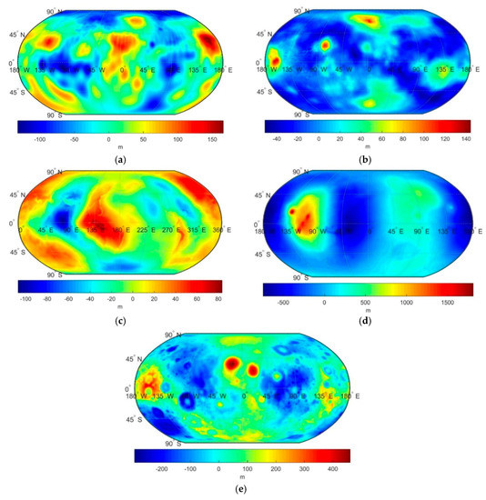
Figure 2.
The quasigeoid models of (a) Mercury, (b) Venus, (c) Earth, (d) Mars and (e) the Moon.
Table 2.
Statistics of the quasigeoid heights on Mercury, Venus, Earth, Mars and the Moon.
Except for some more detailed features, the global quasigeoid patterns on Mercury, Venus, Earth, Mars and the Moon (Figure 2) very closely agree with the geoid patterns on these planetary bodies as presented in Reference [9]. The quasigeoid undulations on Mercury are spatially correlated with major topographic features, having negative values typically in lowlands and positive values in elevated regions (Figure 2a). In addition, the signatures of impact craters could to some extent be recognized. The quasigeoid geometry on Venus is also largely modulated by major topographic features with negative values typically in lowlands. The largest positive values mark the locations of the Alta and Betta Regios volcanic regions and the elevated region of Ishtar Terra (Figure 2b). A prevailing long-wavelength pattern of the quasigeoid geometry on Earth is mainly controlled by deep mantle density heterogeneities (Figure 2c). On Mars, the largest (positive) quasigeoid undulations are in the Tharsis volcanic region with additional localized modifications by the largest volcanic rises of Olympus, Ascraeus, Arsia and Pavonis Mons (Figure 2d). The largest negative values are along the Valles Marineris rift valleys. Large quasigeoid undulations on the Moon are closely spatially correlated with the topography shaped mainly by impact craters (Figure 2e), with the most pronounced maxima in Imbrium and Serenitatis. The largest negative values, on the other hand, mark the locations of the Orientale and South Pole–Aitken impact craters.
3.4. Geoid-To-Quasigeoid Separation
The differences between the geoid and the quasigeoid on Mercury, Venus, Earth, Mars and Moon are shown in Figure 3, with the statistics summarized in Table 3. For completeness, we also plotted the geoid-to-quasigeoid separation values as a function of topographic elevations in Figure 4.
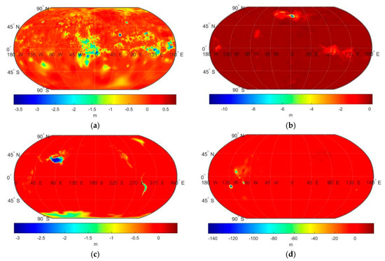
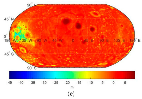
Figure 3.
The geoid-to-quasigeoid separation on (a) Mercury, (b) Venus, (c) Earth, (d) Mars and (e) the Moon.
Table 3.
Statistics of the geoid-to-quasigeoid separation on Mercury, Venus, Earth, Mars and the Moon.
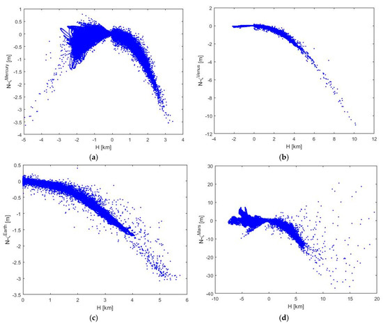
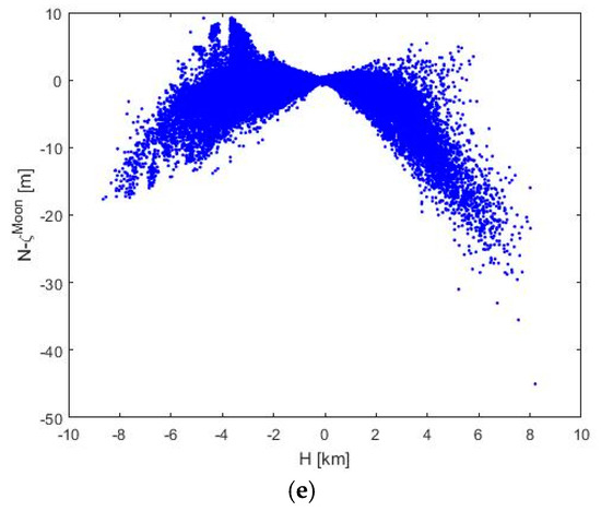
Figure 4.
Spatial correlation between the geoid-to-quasigeoid separation and the topography on (a) Mercury, (b) Venus, (c) Earth, (d) Mars and (e) the Moon.
As seen in Figure 3a, the geoid-to-quasigeoid separation on Mercury is typically negative, with extreme values roughly −3.5 m at the lowest and highest elevations. The differences between the geoid and the quasigeoid increases (non-linearly) with elevations as well as depths (Figure 4a). The geoid-to-quasigeoid separation on Venus is mostly negative, with typically small absolute values not exceeding more than 0.5 m (Figure 3b). The values increase (in the absolute sense) with elevation (Figure 4b) and reach extreme values of −11 m in Ishtar Terra. The differences between the geoid and the quasigeoid on Earth are mostly negative, with the largest negative values in mountainous regions of the Himalayas, Tibet and the Andes, and additional more pronounced differences in Greenland and Antarctica (Figure 3c). The spatial correlation between the geoid-to-quasigeoid separation and the topography on Venus and Earth exhibits a similar trend, but on Earth we see much larger dispersion with respect to a prevailing trend. The largest differences between the geoid and the quasigeoid are observed on Mars. Interestingly, extreme negative as well as positive values of the geoid-to-quasigeoid separation are situated at the highest elevations in the Tharsis region (Figure 3d). Nevertheless, the correlation trend between the geoid-to-quasigeoid separation and the elevations is not clearly manifested (Figure 4d). Large differences are also detected on the Moon, with extreme values of −45 m at the elevated rim of the South Pole–Aitken impact crater (Figure 3e). The spatial correlation between the geoid-to-quasigeoid separation and elevations on the Moon is quite similar to that seen on Mercury, with extreme values at the highest and lowest locations (Figure 4e). This finding is not surprising because these differences correspond to potential differences of values computed on the geoid and the topographic surface.
4. Discussion
In modern geodesy, an undisputable importance of the knowledge of the disturbing potential at the topographic surface has been emphasized both theoretically, in the work of References [3,25] and others, and practically, especially since the arrival of techniques for mapping Earth’s external gravity field from the analysis of orbital parameters of satellites, and the commencement of dedicated satellite gravity missions. Completely disregarding the topographic density information, Molodensky extended this idea further in the definition of normal heights by replacing the mean value of the actual gravity along the plumb line within the topography by the mean value of the normal gravity along the ellipsoidal normal between the telluroid and the reference ellipsoid. This concept is now commonly adopted in many countries for the definition and realization of vertical geodetic datums. In Helmert’s [26] concept, on the other hand, the topographic density information is incorporated in the definition of orthometric heights by computing the mean gravity along the plumb line within the topography approximately according to Poincaré–Prey’s gravity reduction. Helmert’s concept thus represents reality more closely because of the assumption of an average topographic density. Moreover, knowledge of Earth’s upper continental crustal density has improved significantly in recent years, so that the determination of the actual equipotential geometry inside the topography becomes even more realistic, obviously by also taking into consideration the actual topographic geometry.
In planetary sciences, the knowledge of upper crustal density of planetary bodies is still very restricted. Moreover, topographic density information is not needed in the case of negative heights. One could, therefore, argue that in planetary sciences, the use of Molodensky’s concept is more appropriate because positive and negative heights are formally defined with respect to the height reference surface of the quasigeoid that in both cases does not need any density information.
In the definition of orthometric heights, however, this formal consistency is not fulfilled because the density information is used in the case of positive heights compared to zero density in the case of negative heights. Physical heights in this case obviously better represent reality. Furthermore, atmospheric density information could be incorporated for a determination of negative heights in the presence of planetary atmosphere (especially for Venus). From this perspective, the use of density information provides a close representation of reality but is formally inconsistent, and accuracy will depend on the uncertainties of density. In the use of Molodensky’s concept, on the other hand, accuracy depends only on observed quantities (i.e., gravitational and topographic models).
5. Conclusions
The use of density information becomes indispensable in studies of gravity-driven mass movements, where an accurate modelling of the equipotential geometry is required, especially in regions with extreme surface elevation changes such as volcanic rises in the Tharsis region on Mars, or along the rift valleys of Valles Marineris. As seen from our numerical results shown in Figure 3, differences between the geoid and the quasigeoid could even locally exceed 100 m in these places. In this case, Molodensky’s concept introduces relatively large errors that could otherwise be avoided by applying a strict definition of physical height that accounts for topographic density.
Nevertheless, the idea of adopting Molodensky’s concept in planetary studies need not be completely disregarded because of the existence of large surface areas characterized by negative heights. In such cases, topographic density information is irrelevant, which is fully consistent with Molodensky’s main principle of completely disregarding density information. Moreover, information about the crustal density of planetary bodies is still insufficient.
Author Contributions
Conceptualization, R.T.; Methodology, R.T.; Software, I.F.; Validation, I.F.; Formal Analysis, I.F.; Investigation, I.F.; Writing-Original Draft Preparation, R.T.; Writing-Review and Editing, R.T.; Visualization, I.F.
Funding
This research was funded by the Hong Kong Research Grants Council, Project 1-ZE8F: Remote-sensing data for studying the Earth’s and planetary inner structure.
Conflicts of Interest
The authors declare no conflicts of interest. The funders had no role: in the design of the study; in the collection, analyses, or interpretation of data; in the writing of the manuscript; and in the decision to publish the results.
References
- Gauss, C.F. Bestimmung des Breitenunterscchiedes Zwischen den Sternwarten von Gottingen und Altona; Vandenhoeck und Ruprecht: Gottingen, Germany, 1828. [Google Scholar]
- Stokes, G.G. On the variation of gravity at the surface of the Earth. Trans. Camb. Philos. Soc. 1849, 8, 672–695. [Google Scholar]
- Molodensky, M.S.; Yeremeev, V.F.; Yurkina, M.I. Methods for Study of the External Gravitational Field and Figure of the Earth; Israel Program for Scientific Translation: Jerusalem, Israel, 1962. [Google Scholar]
- Rapp, R.H. Use of potential coefficient models for geoid undulation determination using a spherical harmonic representation of the height anomaly/geoid undulations difference. J. Geod. 1997, 71, 282–299. [Google Scholar] [CrossRef]
- Tenzer, R.; Vaníček, P.; Santos, M.; Featherstone, W.E.; Kuhn, M. The rigorous determination of orthometric heights. J. Geod. 2005, 79, 82–92. [Google Scholar] [CrossRef]
- Tenzer, R.; Hirt, C.H.; Novák, P.; Pitoňák, M.; Šprlák, M. Contribution of mass density heterogeneities to the geoid-to-quasigeoid separation. J. Geod. 2016, 90, 65–80. [Google Scholar] [CrossRef]
- Foroughi, I.; Tenzer, R. Comparison of different methods for estimating the geoid-to-quasigeoid separation. Geophys. J. Int. 2017, 210, 1001–1020. [Google Scholar] [CrossRef]
- Tenzer, R.; Foroughi, I. Effect of the mean dynamic topography on the geoid-to-quasigeoid separation offshore. Mar. Geod. 2018. [Google Scholar] [CrossRef]
- Tenzer, R.; Foroughi, I.; Sjöberg, L.E.; Bagherbandi, M.; Hirt, Ch.; Pitoňák, M. Definition of physical height systems for telluric planets and moons. Surv. Geophys. 2018, 39, 313–335. [Google Scholar] [CrossRef]
- Bruns, H. Die Figur der Erde; Publication des Königl, Preussischen Geodätischen Institutes: Berlin, Germany, 1878. [Google Scholar]
- Sjöberg, L.E. A refined conversion from normal height to orthometric height. Stud. Geophys. Geoaetica 2006, 50, 595–606. [Google Scholar] [CrossRef]
- Pizzetti, P. Sopra il calcolo teorico delle deviazioni del geoide dall’ellissoide. Atti della Reale Accademia delle scienze di Torino 1911, 46, 331. [Google Scholar]
- Somigliana, C. Teoria Generale del Campo Gravitazionale dell’Ellisoide di Rotazione. Mem. Soc. Astron. Ital. 1929, 4, 425. [Google Scholar]
- Sjöberg, L.E. On the downward continuation error at the Earth’s surface and the geoid of satellite derived geopotential models. Bollettino di Geodesia e Scienze Affini 1999, 58, 215–229. [Google Scholar]
- Tenzer, R.; Hirt, C.; Claessens, S.; Novák, P. Spatial and spectral representations of the geoid-to-quasigeoid correction. Surv. Geophys. 2015, 36, 627–658. [Google Scholar] [CrossRef]
- Becker, K.J.; Robinson, M.S.; Becker, T.L.; Weller, L.A.; Edmundson, K.L.; Neumann, G.A.; Perry, M.E.; Sean, C. First global digital elevation model of Mercury. In Proceedings of the 47th Lunar and Planetary Science Conference, The Woodlands, TX, USA, 21–25 March 2016. [Google Scholar]
- Erwan, M.; Genova, A.; Goossens, S.; Lemoine, F.G.; Neumann, G.A.; Zuber, M.T.; Smith, D.E.; Solomon, S.C. The gravity field, orientation, and ephemeris of Mercury from MESSENGER observations after three years in orbit. J. Geophys. Res. Planets 2014, 119, 2417–2436. [Google Scholar]
- Wieczorek, M.A. Gravity and topography of the terrestrial planets. Treatise Geophys. 2015, 10, 153–193. [Google Scholar]
- Konopliv, A.S.; Banerdt, W.B.; Sjogren, W.L. Venus Gravity: 180th Degree and Order Model. Icarus 1999, 139, 3–18. [Google Scholar] [CrossRef]
- Hirt, C.; Rexer, M. Earth2014: 1 arc-min shape, topography, bedrock and ice-sheet models—Available as gridded data and degree-10,800 spherical harmonics. Int. J. Appl. Earth Observ. Geoinform. 2015, 39, 103–112. [Google Scholar] [CrossRef]
- Smith, D.E.; Zuber, M.T.; Solomon, S.C.; Phillips, R.J.; Head, J.W.; Garvin, J.B.; Banerdt, W.B.; Muhleman, D.O.; Pettengill, G.H.; Neumann, G.A.; et al. The global topography of Mars and implications for surface evolution. Science 1999, 284, 1495–1503. [Google Scholar] [CrossRef] [PubMed]
- Konopliv, A.S.; Park, R.S.; Folkner, W.M. An improved JPL Mars gravity field and orientation from Mars orbiter and lander tracking data. Icarus 2016, 274, 253–260. [Google Scholar] [CrossRef]
- Barker, M.K.; Mazarico, E.; Neumann, G.A.; Zuber, M.T.; Haruyama, J.; Smith, D.E. A new lunar digital elevation model from the Lunar Orbiter Laser Altimeter and SELENE Terrain Camera. Icarus 2016, 273, 346–355. [Google Scholar] [CrossRef]
- Lemoine, F.G.; Goossens, S.; Sabaka, T.J.; Nicholas, J.B.; Mazarico, E.; Rowlands, D.D.; Loomis, B.D.; Chinn, D.S.; Neumann, G.A.; Smith, D.E.; et al. GRGM900C: A degree 900 lunar gravity model from GRAIL primary and extended mission data. Geophys. Res. Lett. 2014, 41, 3382–3389. [Google Scholar] [CrossRef] [PubMed]
- Bjerhammar, A. On the boundary Value problem of physical geodesy. Tellus 1969, 4, 451–516. [Google Scholar]
- Helmert, F.R. Die Mathematischen und Physikalischen Theorien der Höheren Geodäsie; Teubner: Leipzig, Germany, 1884; Volume 2. [Google Scholar]


© 2018 by the authors. Licensee MDPI, Basel, Switzerland. This article is an open access article distributed under the terms and conditions of the Creative Commons Attribution (CC BY) license (http://creativecommons.org/licenses/by/4.0/).