Reliable Predictors of Arsenic Occurrence in the Southern Gulf Coast Aquifer of Texas

Abstract

Arsenic contamination of groundwater in the Southern Gulf Coast Aquifer of Texas is a critical public health concern as much of the area is rural in nature with decentralized water supplies. Previous studies have pointed to volcanic deposits as the regional source of arsenic but no definitive or reliable predictors of arsenic maximum contaminant level (MCL) exceedance have been identified. In this study, we have studied the effect of various hydrogeochemical parameters as well as soil and land-use variables on arsenic MCL exceedance using logistic regression (LR) techniques. The LR models display good accuracy of 75% or higher but suffer from a high rate of false negatives, highlighting the challenges in capturing the spatial irregularities of arsenic in this region. Despite not displaying high statistical significance, pH appears to be an important variable in the LR models—its effect on arsenic exceedance is not clear and warrants further investigation. The results of the study also show that groundwater vanadium and fluoride are consistently the only significant variables in the models developed; the positive coefficients for both these elements indicates a common geogenic source for arsenic, fluoride and vanadium, corroborating the findings of earlier studies.

1. Introduction

Exposure to drinking-water supplies contaminated by arsenic has been widely-recognised as one of the most significant human health threats of the last few decades. The effects of such exposure range from increased cancer risks to a plethora of cardiovascular, neurological, dermal and respiratory disorders or diseases [1,2,3,4]. Globally, arsenic levels well in excess of the 10 μg/L standard set by the World Health Organization [5] have been detected in water wells in far-east Asia [6,7,8], South-east Asia [9,10,11,12,13], Latin and South America [14,15,16], Europe [17,18,19], as well as the United States [20,21,22,23,24]. In many of these areas, the arsenic is geogenic in nature but human activities such as pumping and irrigation water return have been implicated in its release and migration from the parent source into groundwater. In fact, several recent studies emphasise that understanding mobilization mechanisms is just as critical as identifying the potential sources of arsenic [25,26,27].

In the United States, groundwater is often the only reliable source of potable water in rural areas due to a variety of socio-economic and hydro-climatic factors. The National Groundwater Association (NGWA) reported that more than 13 million year-round occupied households in the country have their own well [28]. In Texas, 62% of the water used in the state in 2014 was supplied by groundwater [29]. The Ogallala Aquifer and the Gulf Coast Aquifer (henceforth referred to as the GCA) are the two largest aquifers in the state and are characterized by their significant irrigation water withdrawals and elevated arsenic levels. The Texas Water Development Board (TWDB), through its Groundwater Quality Sampling Program sampled more than 10,000 wells over a 20-year period leading up to 2004 and discovered that arsenic concentrations in more than 25% of the water samples exceeded the drinking-water standard of 10 μg/L—most of these samples were from the Ogallala and GCA [30]. The TWDB also publishes (with regular updates) a groundwater database, a compilation of groundwater data from nearly 140,000 water wells reported by public agencies as well as private-well owners across the state. Dissolved arsenic is reported as an ‘infrequent constituent’ or trace element in this database; in the GCA alone, dissolved arsenic levels as high as 202 μg/L have been reported in the recent past (in Duval County).

It is critical to note that water supplies in rural areas overlying the Ogallala and GCA are often decentralized and the resources needed for advanced treatment systems for removal of contaminants such as arsenic may not be readily available. Recent efforts by the United States Department of Agriculture (USDA) and the United States Environmental Protection Agency (USEPA) to aid small-scale public water systems have resulted in installation of arsenic-treatment systems in select cities across the state. Successful arsenic removal technologies, often involving iron-based media for sorption, have been demonstrated in the cities of Wellman, Alvin, Bruni and Freer, all of which except the city of Wellman overlie the Gulf Coast Aquifer [31,32]. However, private well owners are still responsible for their own water-treatment alternatives; these are often limited to disinfection and filtration mechanisms which may not meet the drinking-water standard or maximum contaminant level (MCL) of 10 μg/L. It is must also be noted that the TWDB database is by no means comprehensive—most private well owners neither record nor report water level or quality data to the TWDB.

In general, wells with elevated levels of arsenic are more abundant in the southern portion of the GCA (in Texas), as reported by in a comprehensive study of arsenic occurrence in the state [33]. Several studies have attempted to identify potential sources of arsenic in this region as well as its geochemical controls. Hudak [34] sampled 69 water wells in a six-county study area in the South Texas region and discovered a preponderance of arsenic in the Catahoula formation of the GCA; this is the deepest stratigraphic unit and is overlain by other confining beds as well as productive zones (detailed description of the various distinct stratigraphic units is presented in Section 2.1). However, some wells screened in shallower formations contained high arsenic levels as well, albeit with no correlation between arsenic and well depth. The author concluded that while historical use of arsenical pesticides and defoliants in cotton fields may have contributed to enrichment in the shallower zones, decreased application of such chemicals since the 1980s as well as increased controls by natural geologic sources likely explains the spatial distribution of arsenic. Scanlon et al. [33] suggest that positive, albeit weak (r² ranging from 0.12 to 0.43), correlations between arsenic and other dissolved constituents such as vanadium, molybdenum and boron in this region are indicative of a geologic source rather than an anthropogenic (i.e., agriculture) source. They observed the highest arsenic levels in the Jasper Aquifer, the stratigraphic unit immediately overlying the Catahoula formation and point to volcanic ash deposits as the likely (natural) source. Additionally, they postulate that the effects of land-management practices on cotton fields are limited to a smaller, localized spatial scale.

Similar correlations between arsenic and vanadium, potassium and silica were reported by Gates et al. [35], who limited their focus to the unconfined portions of the GCA where most of the pumping occurs. However, they noted that arsenic correlations with these three chemicals were not strong enough to warrant their use as indicators of contamination and that future drilling activity avoid the Catahoula formation due to its relative abundance of arsenic. Chowdhury et al. [36] analysed arsenic in wells from the Chicot, Evangeline and Jasper aquifers and found the highest concentrations to occur in the Jasper. Within each formation, no spatial or vertical (depth) patterns in arsenic occurrence were discernable. They suggest that arsenic, along with selenium and vanadium likely originated from weathering of volcanoclastic sediments. Higher arsenic observed in areas following the outcrop of the Jasper Aquifer are attributed to local geochemical processes in uranium deposits occurring here. The geologic origin of arsenic is also corroborated by Glenn and Lester [37] who studied water quality data across the entire GCA and found statistically significant correlations between arsenic and vanadium.

As such, it appears from the aforementioned studies that the source (volcanic ash deposits) of arsenic and the aquifer unit where it is most-concentrated is well-understood. However, knowledge of hydro-geochemical variables that influence its spatial and vertical distribution is not conclusive enough to allow these variables to act as reliable indicators or predictors of arsenic occurrence. Additionally, earlier works have focused on the correlation between arsenic occurrence and other variables but the effect of these variables on arsenic occurrence has not been studied using rigorous statistical approaches. The use of logistic regression (LR) for understanding the statistical relationships between the dependent and explanatory variables as well as predicting the probability of target analyte occurrence is well documented in groundwater quality studies [38,39,40]. The objective of this study is, therefore, to develop logistic regression models to predict arsenic exceedance (above the drinking-water standard) in the southern GCA as well as evaluate the relative importance of the explanatory variables chosen to develop this model. We aim to evaluate the relationship between arsenic exceedance and a diverse suite of explanatory variables including hydrological, geochemical, soil, climatic and land-use variables and seek to identify stable predictors, particularly those which are easily-measured or readily available, as surrogate measures. The motivation for the study is the paucity of knowledge of such predictors, as pointed out by Gates et al. [35], as well as the demonstration of suitability of logistic regression for such risk-based regional studies by Venkataraman and Uddameri [27].

2. Materials and Methods

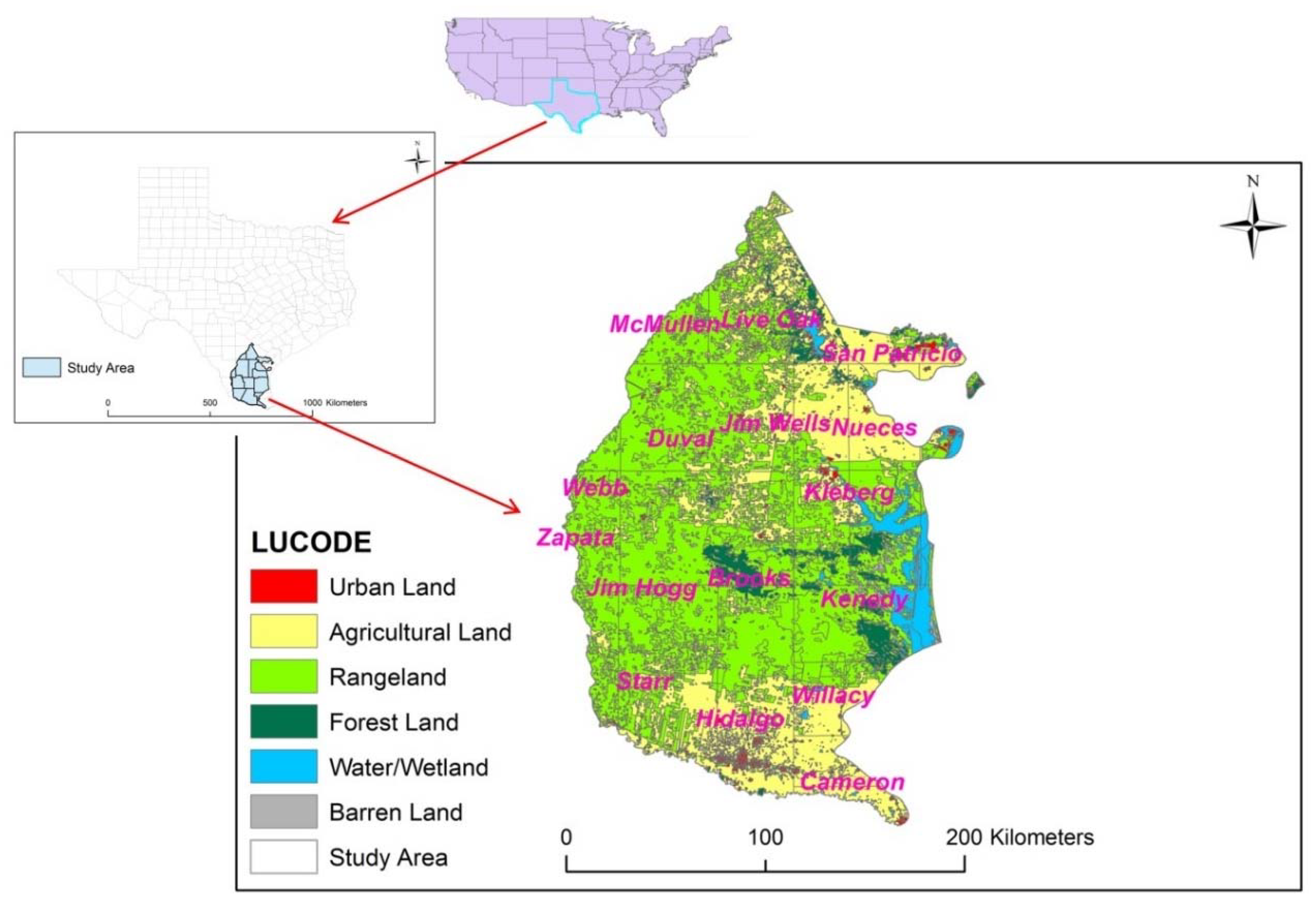
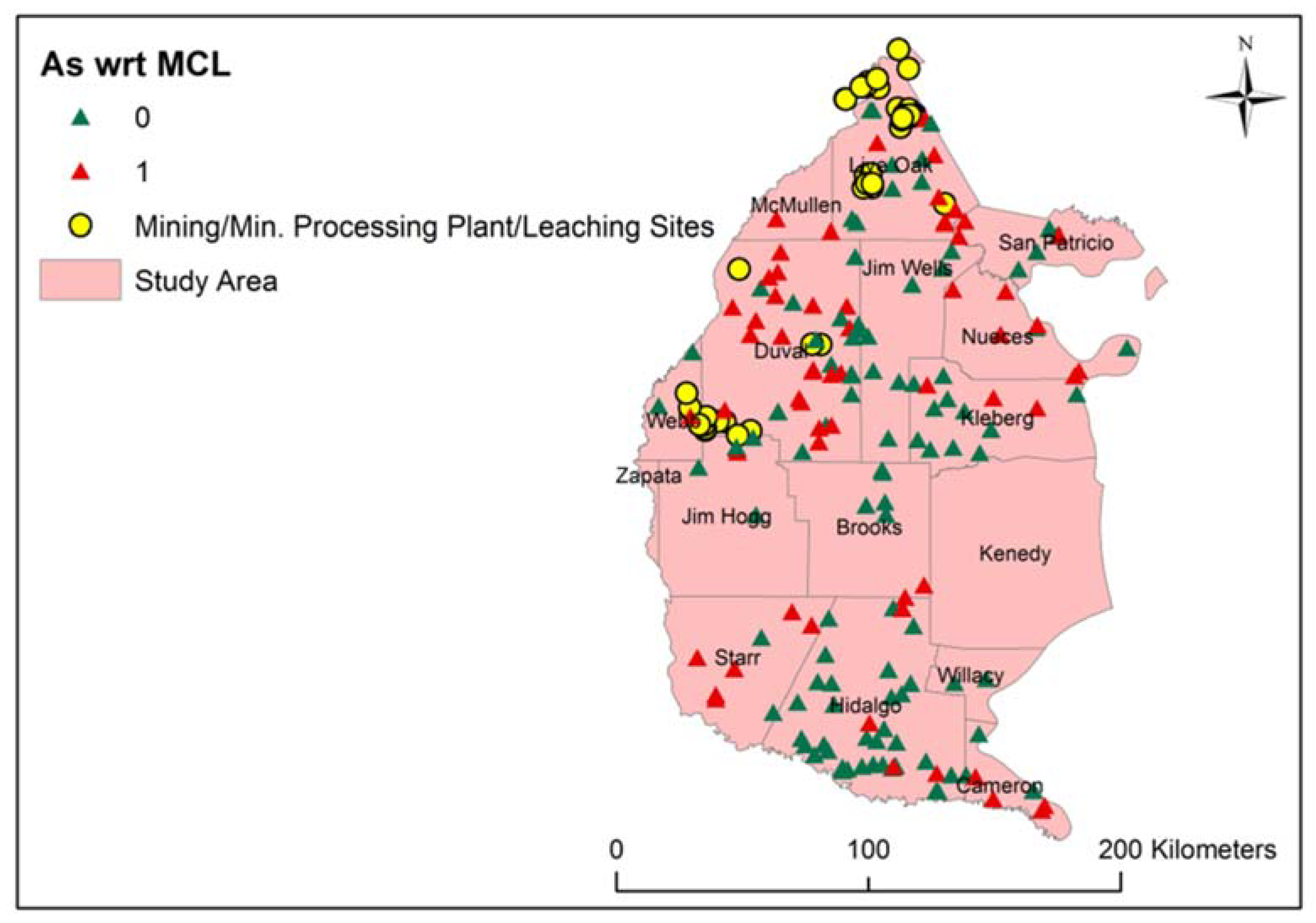
2.1. Study Area Characteristics

Sixteen counties in the southern GCA, as shown in Figure 1, were chosen for the study due to the presence of elevated levels of arsenic reported in the TWDB groundwater database. It must be noted that the northern portion of the GCA in Texas, particularly areas south-west of the City of Houston have recorded high arsenic as well but the number of wells with historically high arsenic levels tend to be concentrated in the southern GCA in Texas. As shown in Figure 1, rangeland and agriculture are the predominant land-use categories in the study area. Rain-fed cotton farming is common in Nueces and San Patricio Counties, while roughly 40% of the counties bordering Mexico (Cameron, Hidalgo and Willacy Counties) are irrigated for cotton production [41]. Other major crops include corn and wheat. Rangeland is comprised of native vegetation used for grazing and livestock—cultivation is generally not practiced here. The rural nature of the area is also evident from this figure.

The GCA in Texas is comprised of five stratigraphic units. From top (youngest) to bottom (oldest), these are: the Chicot Aquifer, the Evangeline Aquifer, the Burkeville confining unit, the Jasper Aquifer, and the Catahoula confining unit [42]. Sediments in the GCA were deposited during the Tertiary and Quaternary periods in ‘steep slopes dipping toward the gulf’, i.e., each of the units generally thickens from east to west, down-dip towards the Gulf of Mexico [36]. Of particular importance is the composition of the Catahoula confining unit—approximately 60% of this unit is made up of volcanic material. Groundwater composition exhibits great spatial variability but, in general, the water is brackish with total dissolved solids’ concentration ranging from 1000 to 10,000 mg/L in the southern GCA. Lower annual precipitation (~500 mm in this region vs. 1300 mm in the northern GCA), higher soil salt accumulations and differences in mineralogy are likely responsible for the saline nature of water in this portion of the GCA. High potential evapotranspiration (PET), as much as two to five times the annual precipitation, has also been indicated as a factor in buildup of salts in the groundwater; these high PET rates also result in recharge rates of <2.5 mm/year [36,43].

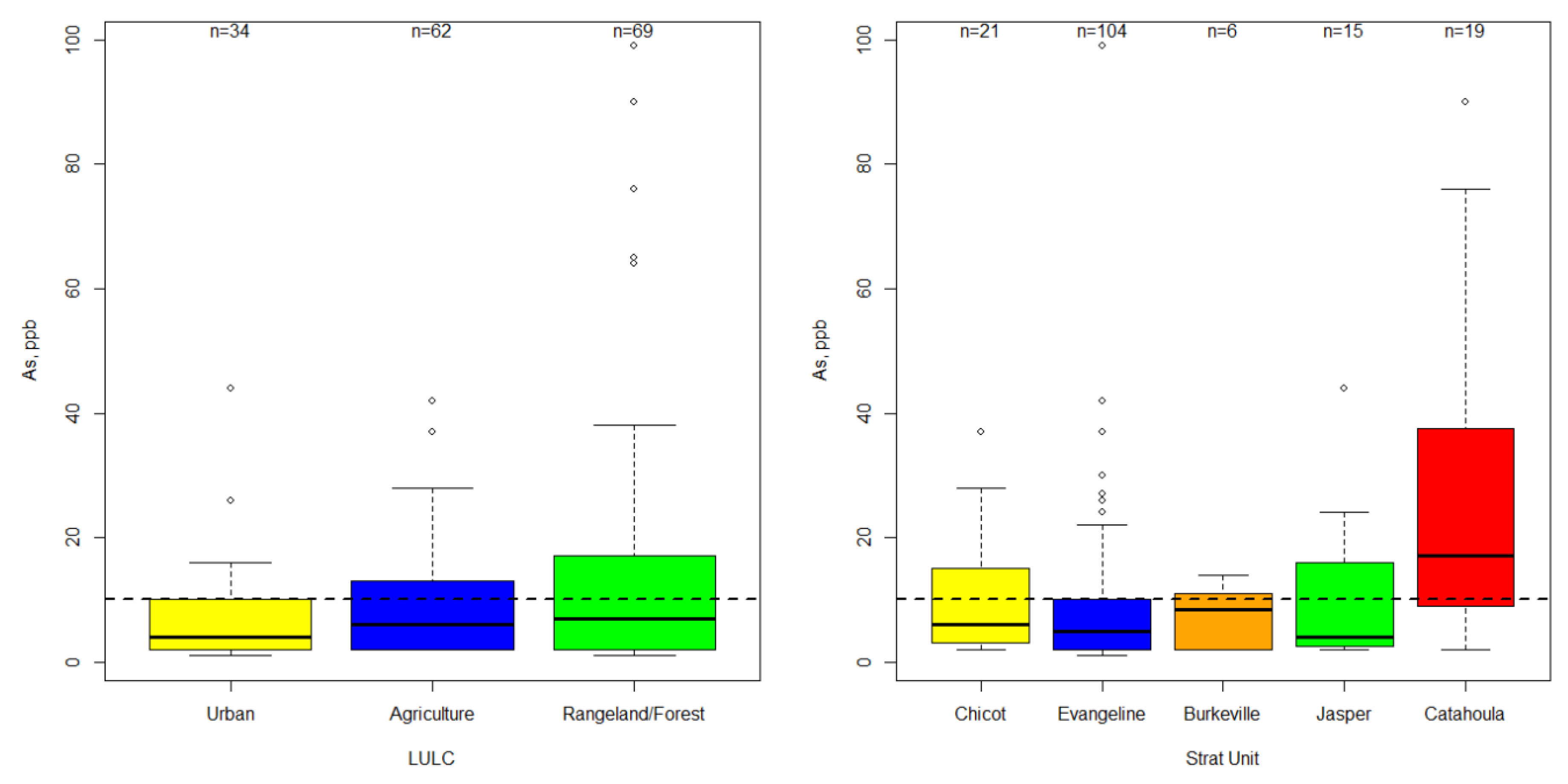
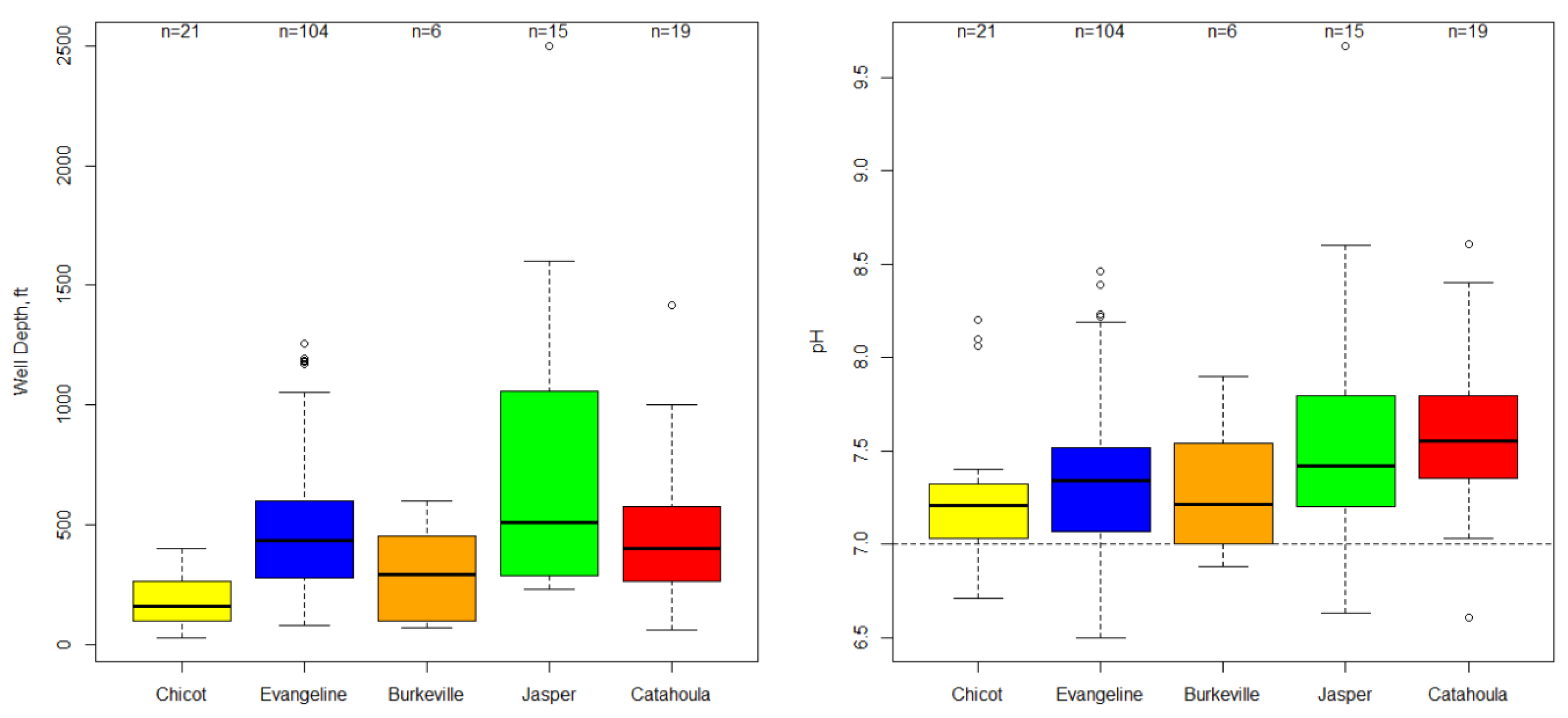
2.2. Data and Selection of Explanatory Variables

The occurrence of arsenic in this region has been largely attributed to natural volcanic deposits by several authors, as discussed in Section 1; the lower-most formation, the Catahoula confining unit, has been identified as the most severely affected. The correlation of arsenic with other volcanically derived materials such as vanadium, selenium, molybdenum, fluoride, potassium and boron, albeit at varying degrees has been documented. The dissolution of arsenic from sulfides or its desorption from iron oxides present in uranium mines near the outcrop area of the aquifer have also been implicated [44]. The potential localized enrichment due to historical application of arsenicals in cotton fields in this region has been pointed out in [33,45]. As indicated by Venkataraman and Uddameri [27], the development of robust LR models to relate arsenic exceedance to other parameters must involve selection of surrogate or explanatory variables that account for various types of sources as well as fate and transport processes. Therefore, the parameters chosen for this study as explanatory variables for building the LR model include (a) well depth and the aquifer unit the well taps into to capture vertical variability; if any (b) groundwater vanadium, potassium, selenium and fluoride to capture association with geogenic sources; (c) land use and groundwater nitrate to capture or simulate the effect of above-ground sources; (d) soil hydrologic group (SHG) and soil organic matter (SOM) to jointly capture the vadose zone fate and transport processes; and (e) relevant major cations and anions to capture other geochemical interactions.

With regard to soil characteristics, SHG is reflective of the infiltration capacity of the soil, which would be pertinent if transport from an above-ground source was involved. SOM (expressed as a percentage) is used to model the adsorptive capacity of soil. The major cations and anions selected were sodium, magnesium, calcium, chloride and sulphate. Of the chosen explanatory variables, the aquifer unit, land use and SHG are categorical in nature while the remainder is continuous. In addition, the pH of the groundwater was included as an explanatory variable as it can influence the solubility, speciation and mobility of arsenic. A key part of the variable selection process was also avoiding the joint assessment of confounding variables which may cloud the true association between those individual variables and the arsenic exceedance. Additionally, the variables were chosen such that redundancy was avoided. In all, 16 variables were selected for testing association with arsenic occurrence and evaluating their inclusion in the eventual LR model. It must be noted that while the association of geogenic arsenic with molybdenum, silica, boron and other trace elements has been reported in other studies, this data is often sparse (or not reported in the groundwater database) and these variables were consequently not included in the study. Likewise, other variables that may exert control on or serve as indicators of arsenic such as oxidation reduction potential or dissolved iron and a variety of soil-related parameters could not be included due to data availability restrictions as well.

Groundwater data for wells located in this 16-county study region was compiled from the TWDB groundwater database. This database is updated daily—however, less than 10% of the wells have current information. Additionally, some of the data presented in this database is not reliable due to various unmet conditions that compromise its quality. Therefore, the wells chosen for the study were selected based on the following criteria: (a) data must not be flagged or coded as unreliable; (b) dissolved arsenic data in the most recent past (between the years 2000 and 2015) must be available; and (c) all other water quality parameters indicated in the previous paragraph (including trace elements such as vanadium and selenium) and hydrogeologic data must be available for wells meeting criteria (a) and (b) for the same time period. Consequently, several wells that had reliable arsenic data were discarded due to the paucity of explanatory variable data. Where multiple records for the same parameter existed for a well over the chosen time period, the most recent sample was used for the study.

On this basis, a total of 165 wells were selected, of which 62 wells had arsenic levels above the MCL. For the purpose of LR modelling, the arsenic concentrations were divided into binary outcomes, labeled 0 or 1, corresponding to non-exceedance or exceedance of the MCL of 10 μg/L, respectively. As mentioned earlier, uranium extraction and mineral processing is common in this region; these plants are mostly clustered in Duval, Live Oak and Webb Counties as shown in Figure 2. In situ leach mining appears to be common practice in many of these plants, as reported in the United States Geologic Survey Mineral Resources Data System [46]. The spatially discontinuous nature of arsenic exceedances is also evident from Figure 2. Many regional studies have reported such spatial irregularities in groundwater arsenic occurrence as well as drinking-water standard exceedances.

Information about the aquifer unit a well taps into or is screened in is also available in the database—these are recorded simply as ‘Gulf Coast Aquifer’ in some instances or on the basis of the aquifer composition, such as ‘Goliad Sand’, ‘Beaumont and Lagarto Clay’, etc. in other cases. The TWDB publishes a Groundwater Availability Model (GAM) which includes the top and bottom depth of each layer or aquifer unit of the Gulf Coast Aquifer in the form of a grid [47]. With the aid of this GAM, the well depth recorded in the database, and the stratigraphic units described by Baker [48], the aquifer unit corresponding to each well was identified and then labeled as either Chicot or Evangeline or Jasper, or as Burkeville confining unit or Catahoula confining unit within a GIS framework. It must be noted that the Burkeville and Catahoula are low-permeability formations, but are nonetheless exploited for human use. For LR purposes, these units were numbered 1 through 5, with 1 representing the top-most unit, the Chicot, and 5 representing the bottom-most or the Catahoula. It can be seen from Figure 3 that 104 of the 165 chosen wells tap into the Evangeline formation; arsenic levels in almost 75% of the wells in the Catahoula exceed the MCL and the highest concentrations occur here as well. All of the 19 wells tapping into the Catahoula are located near the western boundary of the study area in Duval, Live Oak, Starr and Webb Counties whereas those screened in the Chicot are predominantly located near the coast.

All pertinent soil data were compiled for the 16-county study region from the United States Department of Agriculture Soil Survey Geographic Database [49]. SHG and SOM were extracted at each well location using geospatial tools. There are four distinct categories of SHG ranging from Group A to Group D, ranked in order of increasing runoff potential from A to D; much of the study area falls under SHG type B or type C. Group A soils have the highest infiltration rates when wet by virtue of the large composition of sand whereas soils belonging to Group D at the opposite end of the spectrum have the highest runoff potential due to their high clay content and/or shallower depth to water table. To incorporate this parameter into the LR model, it was classified on a scale of 1 to 4, with 1 representing type A soils and 4 representing type D. SOM varied from <1% to 8.5% and showed great spatial variability. Land-use/land-cover (LULC) data was extracted from Lakes Environmental [50]. For LR purposes, LULC was grouped into three categories—(1) land under agriculture, (2) urban, i.e., developed and semi-developed land, including industrial production and (3) rangeland or forestland. This scheme allows for evaluation of the increased or decreased log-odds of arsenic MCL exceedance with reference to the baseline category, assigned to agricultural areas. It must be noted that none of the selected wells were located on barren land and hence this category was not needed. The range of occurrence of arsenic by LULC is presented in Figure 3. It is interesting to note that the highest median arsenic concentration occurs in wells underlying rangeland or forestland areas—in fact, the highest concentrations occur here. However, the results of a Mann–Whitney U test [51] revealed no significant differences in the median concentrations of arsenic between any pair of LULC groups. As some previous studies have pointed out, it is likely that natural volcanic sources underlying these areas may have contributed to arsenic enrichment despite the lack of intensive land-use practices above-ground.

The distributions of well depth and pH with stratigraphic unit are shown in Figure 4. As expected, the shallowest wells are in the Chicot, the top-most layer. The deepest wells are in the Jasper, while wells screened in the Catahoula, the bottom-most formation are located in the western-most boundary of the study region, closer to where it outcrops and thus are not the deepest. The effect of pH on the occurrence, speciation and mobility of arsenic has been well studied (e.g., [7,13]). In general, most trace metals display lower solubility with increasing pH. However, arsenic forms oxyanions in water and higher pH waters tend to have more negatively charged arsenate ions—these ions have a lower tendency to sorb on negatively charged aquifer materials. In our study region, median pH levels generally increase from the Chicot to the Catahoula as shown in Figure 4. This observation is likely due to the effect of weathering of volcanic rocks followed by sustained periods of evaporation in the deeper layers as reported in [34].

Geochemical analysis of the wells revealed that the waters were typically brackish and Na-Cl dominated, likely due to mixing of recharging meteoric water and upward migration of brines from the Yegua–Jackson formation into the Gulf Coast Aquifer as well as dissolution from locally occurring halites [22,33,35,36]. With regards to fluoride, which has been known to co-occur with arsenic where volcanic sources are concerned [14,20,35], the highest median concentrations were observed in the Catahoula. It must be noted that with the exception of one well in this formation, all other selected wells had fluoride levels under the MCL of 4 mg/L. Vanadium concentrations showed similar vertical trends to arsenic—the highest median concentrations were again in the Catahoula. The highest recorded concentration was 400 μg/L in the Evangeline. It must be noted that no MCL exists for vanadium yet—it has been proposed that a notification level of 15 μg/L be set for drinking-water supplies. For the sake of brevity, the Piper trilinear diagrams of the geochemical facies or boxplots showing the distributions of vanadium, fluoride and other selected variables have not been shown here.

2.3. Logistic Regression (LR) Model Development and Evaluation

LR is a commonly-used technique to assess the effect of a set of predictor or explanatory variables on a binary response or outcome. LR is particularly useful when one or more of the explanatory variables are ordinal or categorical in nature. In groundwater studies, it has been used extensively to evaluate the effect of explanatory variables on nitrate and arsenic occurrence above a set threshold, commonly the drinking-water standard (e.g., [27,39,40,52,53,54]). In this study, the exceedance or non-exceedance of arsenic MCL is the chosen response variable. The relationship between probability of exceedance of MCL and the set of chosen explanatory variables is given by Equation (1):

$$\mathrm{p}(As\ge \mathrm{MCL})=\frac{1}{1+\exp (-\mathrm{z})};\mathrm{z}={\beta }_0+{\beta }_1{X}_1+{\beta }_2{X}_2+.....{\beta }_n{X}_n+\epsilon$$

(1)

where p denotes the probability of occurrence of an event—in this case that of arsenic MCL exceedance; β₀ is the intercept, β₁, β₂, …, β_n are the coefficients of n explanatory variables estimated by the maximum likelihood method; X₁, X₂, …, X_n are the explanatory variables; and ε is the random error associated with the model which is assumed to be normally-distributed with a zero mean. An alternate expression for the probability of exceedance takes the logit form as shown in Equation (2):

$$\ln \left(\frac{\mathrm{p}(As\ge \mathrm{MCL})}{\mathrm{p}(As<\mathrm{MCL})}\right)=\ln \left(\frac{\mathrm{p}(As=1)}{\mathrm{p}(As=0)}\right)={\displaystyle \sum _{\mathrm{i}=1}^{\mathrm{n}}{\beta }_{\mathrm{i}}{X}_{\mathrm{i}}}+{\beta }_0+\epsilon$$

(2)

where As = 0 and As = 1 represent the binary outcomes of arsenic (As) MCL exceedance and non-exceedance, respectively. The goal of this modelling process is to develop a parsimonious LR model that contains only those explanatory variables that are statistically significant but also demonstrates the ‘best’ performance as defined by a set of well-defined metrics.

As discussed in Section 2.2, a diverse set of explanatory variables was chosen to develop the LR model. These variables were chosen due to their observational or theoretical relationship with arsenic occurrence reported in earlier studies. The first step in the model development process involved univariate analysis or the assessment of the association between each of the 16 explanatory variables, chosen one at a time, and arsenic exceedance. At this stage, the statistical significance of each variable was evaluated at a less-stringent p value of 0.25 and only those variables that passed this criterion were selected for inclusion in the multivariate LR model. This approach of retaining a select few variables from the originally chosen list of explanatory variables was adopted to avoid an unstable model that had limited applicability, as recommended by Tabachnick and Fiddell [55] and Hosmer et al. [56]. As a general rule-of-thumb, Agresti [57] recommends that for every independent variable, there be no fewer than 10 outcomes in each binary category. Considering that there were 62 exceedances (and 103 non-exceedances), it is desirable to then shortlist the number of explanatory variables to seven or fewer. Similar recommendations have been made by Peduzzi et al. [58] to avoid overfitting or underfitting the model.

The next step in the LR model development is the selection of the model validation method. Several methods have been prescribed in the literature, including, (a) the separation of the dataset into training subset to first build the model, and testing subsets to validate it; (b) k-fold cross-validation (CV) involving splitting the dataset into k-number of (roughly) equally-sized subsets for model development and validation; (c) a computationally more-expensive version of the k-fold CV, known as the leave-one-out-cross-validation or LOOCV; and (d) bootstrapping with replacement [59,60,61,62]. The suitability and limitations of these approaches have been well studied, albeit with no general consensus or recommendations (e.g., [63,64,65,66]). In this study, we have adopted a variant to the k-fold CV approach for model testing by randomly splitting the dataset into training (95%) and testing (5%) 500 times. It must be noted that this approach was thoroughly tested against the LOOCV as well as bootstrap approaches to ensure model underfitting, overfitting or paradoxical error did not occur.

Various metrics were used to evaluate the LR model. The commonly used Hosmer–Lemeshow goodness-of-fit test was used as an overall measure of model fit. Model performance was evaluated using receiver operating characteristics (ROC). Specifically, the area under the ROC curve (AUC) and various parameters defined by Fawcett [67] including the true positive rate (TPR), false positive rate (FPR), true negative rate (TNR), false negative rate (FNR), positive predictive value (PPV), negative predictive value (NPV) and overall accuracy (calculated as shown in Equations (3)–(9)) were used as a measure of predictive capacity of the model:

$$\mathrm{TPR}=\frac{{\displaystyle \sum \mathrm{TP}}}{{\displaystyle \sum \mathrm{TP}+\mathrm{FN}}}$$

(3)

$$\mathrm{FPR}=\frac{{\displaystyle \sum \mathrm{FP}}}{{\displaystyle \sum \mathrm{FP}+\mathrm{TN}}}$$

(4)

$$\mathrm{PPV}=\frac{{\displaystyle \sum \mathrm{TP}}}{{\displaystyle \sum \mathrm{TP}+\mathrm{FP}}}$$

(5)

$$\mathrm{NPV}=\frac{{\displaystyle \sum \mathrm{TN}}}{{\displaystyle \sum \mathrm{TN}+\mathrm{FN}}}$$

(6)

$$\mathrm{TNR}=1-\mathrm{FPR}$$

(7)

$$\mathrm{FNR}=1-\mathrm{TPR}$$

(8)

$$\mathrm{Accuracy}=\frac{{\displaystyle \sum \mathrm{TP}+\mathrm{TN}}}{\mathrm{Population}\mathrm{Size}}$$

(9)

In the above equations, TP is the number of true positives, TN is the number of true negatives, FP is the number of false positives, FN is the number of false negatives and the total number of data points is the population size. Use of these ROC diagnostics have been prescribed for studies when determining cut-off points to optimize classification accuracy are involved; these measures can be calculated once a 2 × 2 contingency table comparing the true observations and model-predicted outcomes has been generated. The statistical significance of each variable was determined using the p value of the chi-squared test [68]. Additionally, the likelihood ratio test (LRT) was used to assess whether individual predictors contributed significantly to the model, an approach recommended by Hilbe [69].

The steps listed above were followed to build three separate LR models—(a) one for the entire dataset, henceforth referred to as the master LR model; (b) one for the wells tapping into the top two layers and thus representing the unconfined formation, henceforth referred to as the unconfined LR model; and (c) one for only those wells tapping into the Evangeline Aquifer which had the most number of wells (104) in our dataset, henceforth referred to as the Evangeline LR model. The motivation for building additional models limited to the unconfined formations and Evangeline was to comparatively assess the predictive capacity of the model as well as attempt to investigate characteristics that may be unique to the unconfined layers. All model development, assessment and metrics evaluation were conducted in an R environment [70].

3. Results

It was determined that the following variables did not display any statistical significance to merit inclusion in the model development process: dissolved calcium, magnesium, sodium, chloride, sulphate, nitrate, selenium, SOM, SHG and LULC. Thus, these variables have been omitted from the rest of the article.

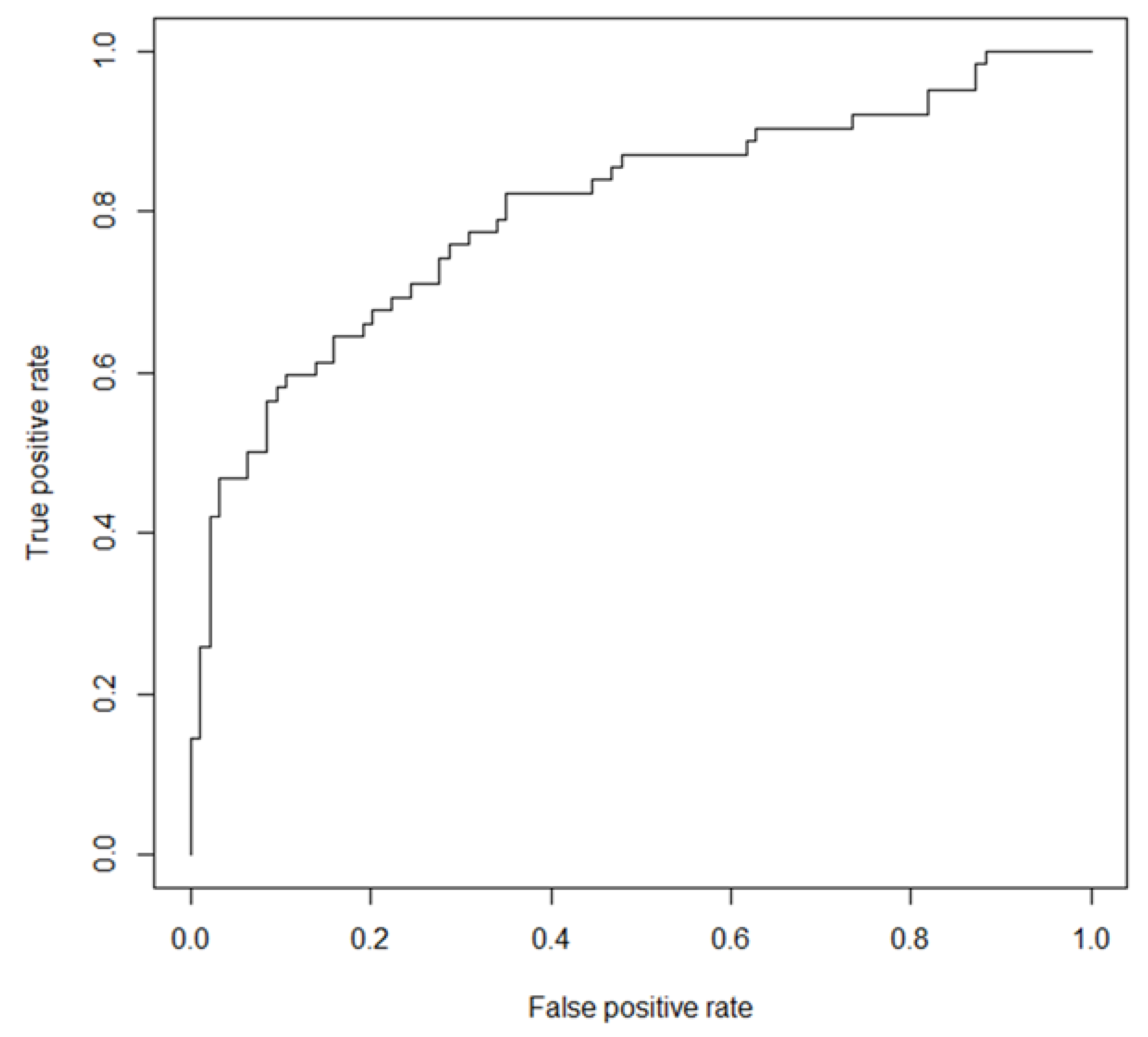
3.1. Performance of the Master LR Model

Univariate analysis of the explanatory variables showed that only aquifer stratigraphic unit, pH, fluoride and vanadium were significant at p < 0.25. The master LR model was then cross-validated and built using these variables. The coefficients for each of the variables in this model as well as their associated p values are shown in the model summary section of

Table 1. Summary of the master logistic regression (LR) model (significant variables at p ≤ 0.05 are shown in bold and asterisk).

Model Summary				Likelihood Ratio Test (LRT) Results Summary
Parameter	Estimate	Std. Error	p-Value	Parameter	Deviance	Pr (>Chi)
Intercept	2.1414	1.7188	0.2128	NULL	209.65	-
F *	0.6572	0.3096	0.0338	F *	200.73	0.0028
Aq Strat Unit 2	−1.0517	0.5853	0.0723	Aq Stat Unit *	189.47	0.0327
Aq Strat Unit 3	−1.6687	1.2302	0.1750
Aq Strat Unit 4	0.4209	0.8028	0.5997
Aq Strat Unit 5	0.7737	0.8462	0.3606
pH	−0.5065	0.2348	0.0551	pH *	181.93	0.0042
V *	0.0461	0.0098	<1 × 10−4	V *	156.66	<1 × 10−6

. It can be seen that fluoride and vanadium alone show statistical significance at p < 0.05.

Both fluoride and vanadium have positive regression coefficients, suggesting a common volcanic source. It must also be noted that the coefficient for vanadium displays much higher statistical significance than fluoride. The results of the LRT (shown in Table 1) indicate that all variables, including pH, must be retained in the model. It is interesting to note that although the coefficient for pH was not statistically significant (only marginally above the threshold of 0.05), its contribution to the model is. The same statement is true of aquifer stratigraphic unit as well, which seems to indicate a (weak) decreased logit of arsenic exceedance in the Evangeline relative to the Chicot.

The ROC curve for the master LR model is shown in Figure 5 and the ROC metrics are summarized in

Table 2. Comparison of model ROC performance characteristics.

Parameter	Master LR	Unconfined LR	Evangeline LR
Accuracy	0.7628	0.7458	0.7959
True Positive Rate	0.5645	0.4250	0.5455
False Positive Rate	0.1064	0.0897	0.0769
True Negative Rate	0.8936	0.9103	0.9231
False Negative Rate	0.4355	0.5750	0.4545
Positive Predictive Value	0.7778	0.7083	0.7826
Negative Predictive Value	0.7568	0.7553	0.8000

. The AUC is 0.80—for comparison, a model that is no better than a random guess (the outcome of tossing a coin is often used as an example here) would produce an AUC of 0.5, following a diagonal from the origin to (1,1). Fawcett [67] notes that points further ‘north-west’ of this diagonal or to the left of this graph are more conservative as they have low true positive rates as they do not make positive classifications unless strong evidence is present. This is reflected in the relatively-poor TPR of the model (0.5645) shown in Table 2. Consequently, the FNR, which is calculated as 1-TPR, is 0.4355, indicating that the model is incorrectly classifying a large number of observed exceedances as non-exceedances. From a risk-minimization perspective, an ideal model would have a small FNR particularly if the goal is to prevent exposure. Nonetheless, the overall accuracy of the model is 0.7628, or 76.28%. The p-value for the Hosmer–Lemeshow goodness-of-fit test was 0.42, indicating that the null hypothesis of the model being a good fit was to be retained.

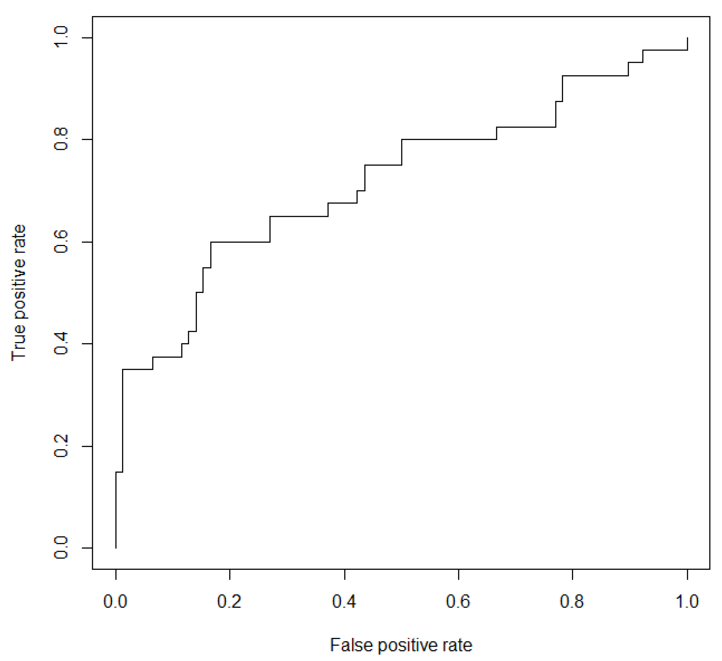
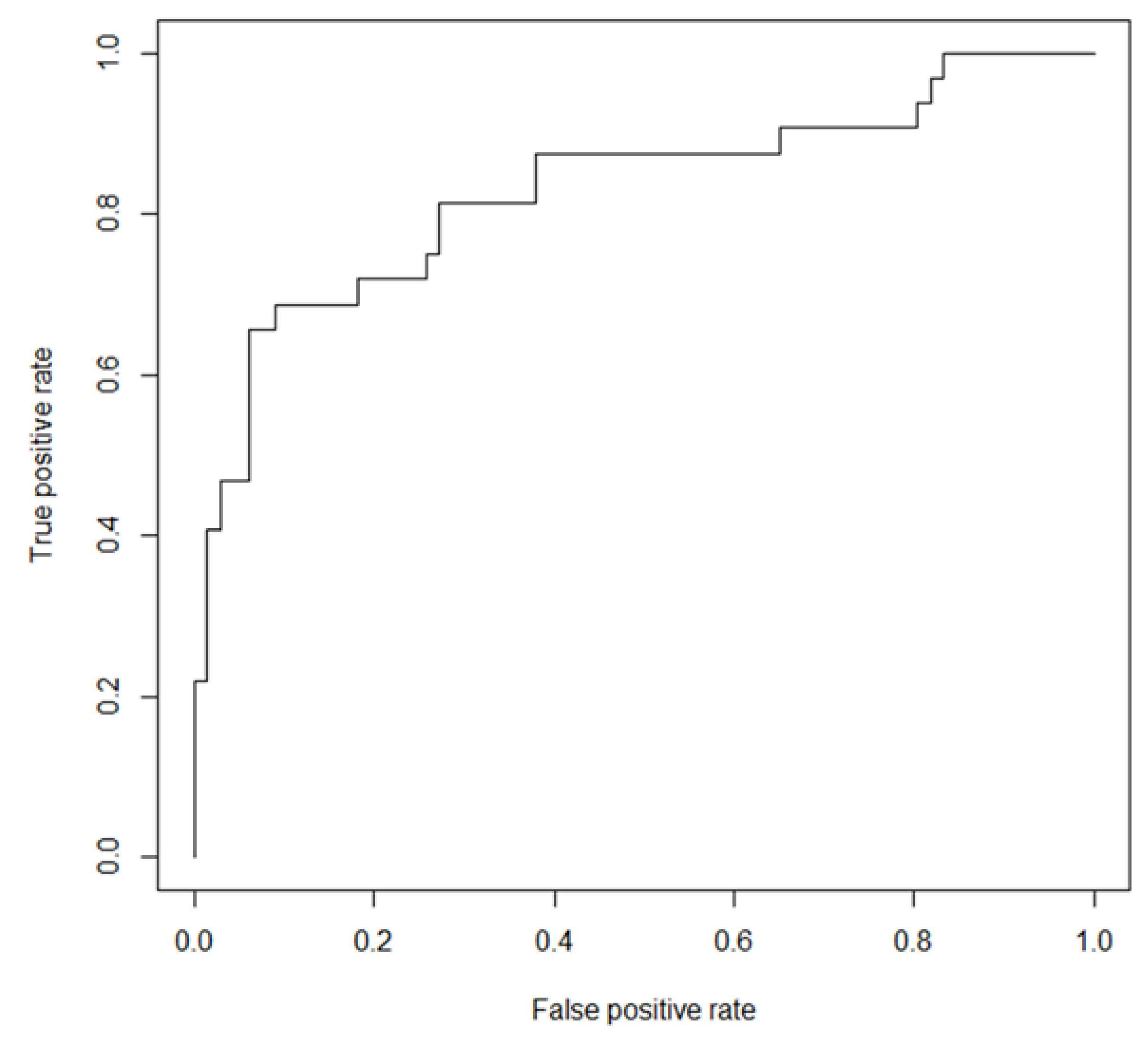
3.2. Performance of the Unconfined and Evangeline LR Models

There are 125 wells in our dataset in the Chicot and Evangeline formations, of which 21 are in the Chicot—these were used to develop the unconfined LR model. Univariate analysis of the unconfined LR model showed that pH, fluoride, vanadium and well depth were significant at p < 0.25. A summary of the statistical significance of these variables in the resulting model is presented in

Table 3. Summary of the unconfined LR model (significant variables at p ≤ 0.05 are shown in bold and asterisk).

Model Summary				LRT Results Summary
Parameter	Estimate	Std. Error	p-Value	Parameter	Deviance	Pr (<Chi)
Intercept	0.9843	1.6711	0.5585	NULL	151.12	-
F *	0.6921	0.3292	0.0355	F *	146.56	0.0325
Well Depth	−0.0007	0.0345	0.4533	Well Depth	146.34	0.2344
pH	−0.4450	0.2364	0.0597	pH *	140.89	0.0172
V *	0.0349	0.0104	<1 × 10−3	V *	127.36	<1 × 10−3

. As was observed in the master LR model, vanadium and fluoride were the most statistically significant variables, both with positive coefficients. Once again, none of the variables that are suggestive or indicative of (human) above-ground inputs showed any statistical significance. As was observed in the master LR, pH shows a negative regression coefficient, albeit with a p-value of only marginally above the 0.05 threshold. The LRT indicates that the variables that contribute most to the reduction in deviance of the model are pH, fluoride and vanadium, despite pH’s regression coefficient not displaying statistical significance.

The unconfined LR model had the poorest performance in terms of ROC diagnostics of the three models developed. The ROC curve for this model is shown in Figure 6 and the AUC is 0.72. While the overall accuracy of this model is good (74.58%), it suffers from a high rate of false negatives (57.50%) as shown in Table 2. This indicates that over half of the wells where exceedance was observed were incorrectly classified as non-exceedances. This model also has the lowest TPR (42.50%). However, as was the case with the master LR, the unconfined LR model passed the Hosmer–Lemeshow goodness-of-fit test as well.

A summary of the Evangeline LR model characteristics is shown in

Table 4. Summary of the Evangeline LR model (significant variables at p ≤ 0.05 are shown in bold and asterisk).

Model Summary				LRT Results Summary
Parameter	Estimate	Std. Error	p-Value	Parameter	Residual Deviance	Pr (<Chi)
Intercept	−0.2339	1.1887	0.8440	NULL	123.81	-
pH	−0.3175	0.1752	0.0699	pH	122.33	0.2237
F	0.6476	0.3894	0.0966	F *	115.61	0.0168
V *	0.0473	0.0111	<1 × 10−3	V *	99.34	<1 × 10−4

. Vanadium was the only statistically significant variable with a positive coefficient again. However, the LRT shows that both fluoride and vanadium contribute significantly to reduction in deviance of the model. It is interesting to note that the p value of the regression coefficients for pH is again negative and only marginally-above the chosen threshold. The master LR and unconfined LR models displayed similar characteristics in terms of pH.

The AUC for the Evangeline LR (see Figure 7) was 0.82, a marginal improvement over the AUC of the master LR model treated earlier. However, this model has a very good accuracy of 79.69%, a marked improvement over both the master and unconfined LR models, as shown in Table 2. It can also be seen that the Evangeline LR outperforms the other two models in all other categories except the TPR and FNR. The Evangeline LR model also passed the Hosmer–Lemeshow goodness-of-fit test.

4. Discussion

Groundwater contamination with arsenic has proved to be one of the biggest challenges in public health management in rural areas. The general lack of reliable predictors of elevated levels of arsenic in the Gulf Coast Aquifer has been highlighted in earlier works; the highly irregular spatial nature of its occurrence has also been emphasised. Therefore, the identification of variables which are relatively easy to measure or data for which is readily available that may act as a surrogate or indicator of arsenic exceedance is critical. It appears from the three LR models developed in this study that dissolved vanadium is consistently the variable with the highest statistical significance as well as the parameter of utmost importance in terms of its contribution to model performance. Several earlier works [23,33,34,35,36,37] have documented the correlation of arsenic with vanadium in the Ogallala Aquifer and Gulf Coast Aquifer; arsenic in both these systems is suspected of having the same origin (volcanoclastic sediments). In the Gulf Coast Aquifer itself, positive correlations of arsenic with vanadium (r² as high as 0.43) have been recorded, leading to the consensus that natural geologic sources are involved. In this study, we have built on this information by using variables such as vanadium for binary classification purposes and have demonstrated the positive nature of its logistic regression coefficient as well as its high statistical significance, thus corroborating the results of earlier works. Despite the spatial irregularities in arsenic occurrence, vanadium is nonetheless a significant variable in the LR models everywhere, suggesting a regional source of arsenic, likely volcanic deposits. As such, there are several other interesting and significant findings that provide insight into the mechanisms of arsenic occurrence that are discussed below.

While vanadium is evidently the most statistically significant variable, its practical use as a predictor is limited by the cost of its measurement—if dissolved vanadium levels are being sought, one could just as easily test the same sample for arsenic and other dissolved metals as well. Thus, from a variable selection perspective, it is critical to note the importance of fluoride in each of the three models presented. Similar to the stratigraphic distribution of arsenic, the highest concentrations of fluoride are also found in the Catahoula (figure not shown). If we consider the master LR and unconfined LR models, fluoride has the highest (positive) coefficient indicating the strong control it exerts on arsenic. As mentioned earlier, exploration of the relationship between arsenic and other ionic species such as fluoride in earlier studies has been limited to correlation coefficients—we have shown in this study that fluoride can serve as a reliable predictor of arsenic as well, at least as far as the region, in general, or the unconfined formations, in isolation, are considered.

The relationship between pH and the arsenic logit merits discussion as well. Along with vanadium and fluoride, pH was the only variable to feature in each of the three models. It is interesting to note that its inclusion in these models is warranted, as evidenced by the LRT, despite the statistical insignificance of its regression coefficients. If we were to relax even marginally our rejection criterion (of p < 0.05), pH would be included in all three models. pH also consistently displays a negative coefficient indicating increased odds of arsenic exceedance with pH decrease. This is rather anomalous, considering that current literature reports arsenic levels in groundwater impacted by volcanic activity generally increase with pH (up to 8.5) (e.g., [15,71] etc.) Additionally, it has been shown that higher pH tends to limit arsenic adsorption in saline groundwaters [20]. As such, more investigation of the pH control on arsenic is recommended; this would require knowledge of other variables, particularly redox and sorption conditions, and environments as well as that of other dissolved species that may encourage arsenic dissolution. Other treatment methods, which are discussed later in this section may also help uncover this contradictory behavior.

The effect of land-use practices, namely agriculture and uranium extraction operations, are not conclusive from this study. It was pointed out earlier that the highest arsenic concentrations actually occur on rangeland and forestland, albeit with no statistically significant difference in median arsenic levels between wells associated with these two areas. LULC was not a significant variable even during the univariate analysis phase. Hudak [34] suggested that the effect of arsenical pesticides applied on cotton farmlands in this area prior to the 1990s has likely diminished due to decreased use of such chemicals as well as ‘stronger controls exerted’ by geogenic sources. Although well depth did not play a significant role in the unconfined model, it was originally shortlisted because it had met the less-stringent critieria of p < 0.25 in the univariate analysis phase (it had a p value of 0.09 when treated singularly). Thus, the possibility of a land source, albeit with a much weaker effect, cannot be entirely ruled out, at least as far as the top two layers are concerned. Some recent studies such as Podgorski et al. [72] have encouraged the use of irrigated acreage as a stronger variable than the categorical LULC variable we have used. However, this data was not readily available. A review of the USDA Mineral Resource Data System showed that all plants associated with uranium mining or processing were limited to Duval, Live Oak and Webb Counties. These plants appear to have largely been operational prior to the 1990s—some of these plants were still active in the early 21st century. It has been reported that open-pit mining as well as solution mining were the commonly employed uranium exploitation methods here [33,35] Given the spatial clustering of these plants and the higher number of arsenic exceedances in these three counties, as shown in Figure 2, it appears that the effect of such extraction and processing is likely limited to a smaller spatial scale as opposed to providing an explanation for arsenic distribution on a regional scale. More advanced geospatial methods statistical techniques of exploring this relationship in these counties are warranted.

As far as the model performance metrics are concerned, it is evident that all three models have relatively high FNRs, indicating that they are unable to correctly classify the observed exceedances. In particular, the performance of the unconfined LR model in relation to the other two models, especially the Evangeline, is diminished. It is likely that the spatial variability in arsenic in the Chicot, the top-most layer is far too complex for the unconfined LR to capture adequately. However, when the other wells are included, i.e., the master LR model, the performance improves marginally and when the Chicot wells are removed to produce the Evangeline LR, the performance improves markedly. As such, this finding suggests that a lumped approach of modelling occurrence without distinguishing between the aquifer unit may not be prudent. Considering that majority of the wells in the Southern Gulf Coast tap into the Evangeline (not just in our study but as a sweeping statement), it is recommended that these wells be treated uniquely. Their FNRs notwithstanding, both the master LR and the Evangeline LR models display good accuracy, in excess of 75%.

We also acknowledge some of the limitations of our study. The primary objective of this study was the identification of reliable predictors of arsenic exceedance using LR techniques alone—thus, we have paid limited attention to exploration of transport and mobilization mechanisms from a mass balance perspective. We are also constrained by the limitations in data availability. The inclusion of other oxyanion-forming variables such as molybdenum, dissolved species like uranium and silica, as well as redox indicators would likely have not only enhanced the performance of the models but also aided in the explanation of some of the transport/mobilization mechanisms—however, this data is sparse. With regard to the data used in the study, the groundwater data used is reflective of the most recent records available in the TWDB database; this database relies on reporting from various local groundwater conservation districts as well as self-reporting from private owners. While we have been extremely cautious in selecting reliable data alone, we acknowledge the uncertainty therein. The authors also acknowledge recent developments in risk-modelling and variable importance investigations. We are aware of recent studies [73,74,75,76] that have demonstrated the applicability of artificial neural networks, k-nearest neighbours, and random forests in modelling groundwater contamination risks. Considering that the LR models we have developed, despite their good overall accuracy, were still deficient in their false negative rates, it is suggested that the aforementioned statistical frameworks be considered for evaluation and comparison in our study region.

5. Conclusions

In conclusion, arsenic occurrence at elevated levels in the Southern Gulf Coast Aquifer of Texas is an urgent public health concern considering the rural nature of this area. Water supplies in many of these areas are decentralized and the need to identify arsenic ‘hot spots’ using surrogate measures is critical. The LR models developed in this study show that vanadium and fluoride exert the largest control on arsenic occurrence in the area and that fluoride on its own can be used as a reliable predictor. As such, volcanic deposits appear to be the regional source of groundwater arsenic, but on smaller spatial scales other factors may be responsible for localized arsenic enhancement. Considering the differences in the performances of the three models developed, it is recommended that arsenic occurrence in the Evangeline formation, where most of the wells are screened, be treated separately. We have found the highest arsenic concentrations to occur in the Catahoula, pumping from which appears to be common along the western boundary of the study region where it outcrops. We recommend that exploitation of this formation for drinking-water purposes be avoided.

References

1. Abernathy, C.O.; Liu, Y.P.; Longfellow, D.; Aposhian, H.V.; Beck, B.; Fowler, B.; Waalkes, M. Arsenic: Health effects, mechanisms of actions, and research issues. Environ. Health Perspect. 1999, 107, 593. [Google Scholar] [CrossRef] [PubMed]
2. Yoshida, T.; Yamauchi, H.; Sun, G.F. Chronic health effects in people exposed to arsenic via the drinking water: Dose-response relationships in review. Toxicol. Appl. Pharmacol. 2004, 198, 243–252. [Google Scholar] [CrossRef] [PubMed]
3. Duker, A.A.; Carranza, E.; Hale, M. Arsenic geochemistry and health. Environ. Int. 2005, 31, 631–641. [Google Scholar] [CrossRef] [PubMed]
4. Naujokas, M.F.; Anderson, B.; Ahsan, H.; Aposhian, H.V.; Graziano, J.H.; Thompson, C.; Suk, W.A. The broad scope of health effects from chronic arsenic exposure: Update on a worldwide public health problem. Environ. Health Perspect. 2013, 121, 295. [Google Scholar] [CrossRef] [PubMed]
5. World Health Organization. Arsenic Fact Sheet. Available online: http://www.who.int/mediacentre/factsheets/fs372/en/ (accessed on 22 January 2018).
6. Shim, M.J.; Kim, H.J.; Yang, S.J.; Lee, I.S.; Choi, H.I.; Kim, T.U. Arsenic trioxide induces apoptosis in chronic myelogenous leukemia K562 cells: Possible involvement of p38 MAP kinase. BMB Rep. 2002, 35, 377–383. [Google Scholar] [CrossRef]
7. Guo, H.; Yang, S.; Tang, X.; Li, Y.; Shen, Z. Groundwater geochemistry and its implications for arsenic mobilization in shallow aquifers of the Hetao Basin, Inner Mongolia. Sci. Total Environ. 2008, 393, 131–144. [Google Scholar] [CrossRef] [PubMed]
8. Rodríguez-Lado, L.; Sun, G.; Berg, M.; Zhang, Q.; Xue, H.; Zheng, Q.; Johnson, C.A. Groundwater arsenic contamination throughout China. Science 2013, 341, 866–868. [Google Scholar] [CrossRef] [PubMed]
9. Neumann, R.B.; Ashfaque, K.N.; Badruzzaman, A.B.M.; Ali, M.A.; Shoemaker, J.K.; Harvey, C.F. Anthropogenic influences on groundwater arsenic concentrations in Bangladesh. Nat. Geosci. 2010, 3, 46. [Google Scholar] [CrossRef]
10. Flanagan, S.V.; Johnston, R.B.; Zheng, Y. Arsenic in tube well water in Bangladesh: Health and economic impacts and implications for arsenic mitigation. Bull. World Health Organ. 2012, 90, 839–846. [Google Scholar] [CrossRef] [PubMed]
11. Rahman, M.M.; Dong, Z.; Naidu, R. Concentrations of arsenic and other elements in groundwater of Bangladesh and West Bengal, India: Potential cancer risk. Chemosphere 2015, 139, 54–64. [Google Scholar] [CrossRef] [PubMed]
12. Aziz, Z.; Van Geen, A.; Stute, M.; Versteeg, R.; Horneman, A.; Zheng, Y.; Hoque, M.A. Impact of local recharge on arsenic concentrations in shallow aquifers inferred from the electromagnetic conductivity of soils in Araihazar, Bangladesh. Water Resour. Res. 2008, 44. [Google Scholar] [CrossRef]
13. Mukherjee, A.; von Brömssen, M.; Scanlon, B.R.; Bhattacharya, P.; Fryar, A.E.; Hasan, M.A.; Sracek, O. Hydrogeochemical comparison and effects of overlapping redox zones on groundwater arsenic near the Western (Bhagirathi sub-basin, India) and Eastern (Meghna sub-basin, Bangladesh) margins of the Bengal Basin. J. Contam. Hydrol. 2008, 99, 31–48. [Google Scholar] [CrossRef] [PubMed]
14. Armienta, M.A.; Segovia, N. Arsenic and fluoride in the groundwater of Mexico. Environ. Geochem. Health 2008, 30, 345–353. [Google Scholar] [CrossRef] [PubMed]
15. Bundschuh, J.; Litter, M.I.; Parvez, F.; Román-Ross, G.; Nicolli, H.B.; Jean, J.S.; Cuevas, A.G. One century of arsenic exposure in Latin America: A review of history and occurrence from 14 countries. Sci. Total Environ. 2012, 429, 2–35. [Google Scholar] [CrossRef] [PubMed]
16. George, C.M.; Sima, L.; Arias, M.; Mihalic, J.; Cabrera, L.Z.; Danz, D.; Gilman, R.H. Arsenic exposure in drinking water: An unrecognized health threat in Peru. Bull. World Health Organ. 2014, 92, 565–572. [Google Scholar] [CrossRef] [PubMed]
17. Aiuppa, A.; D’Alessandro, W.; Federico, C.; Palumbo, B.; Valenza, M. The aquatic geochemistry of arsenic in volcanic groundwaters from southern Italy. Appl. Geochem. 2003, 18, 1283–1296. [Google Scholar] [CrossRef]
18. Cinti, D.; Poncia, P.P.; Brusca, L.; Tassi, F.; Quattrocchi, F.; Vaselli, O. Spatial distribution of arsenic, uranium and vanadium in the volcanic-sedimentary aquifers of the Vicano-Cimino Volcanic District (central Italy). J. Geochem. Explor. 2015, 152, 123–133. [Google Scholar] [CrossRef] [Green Version]
19. Katsoyiannis, I.A.; Mitrakas, M.; Zouboulis, A.I. Arsenic occurrence in Europe: Emphasis in Greece and description of the applied full-scale treatment plants. Desalin. Water Treat. 2015, 54, 2100–2107. [Google Scholar] [CrossRef]
20. Welch, A.H.; Westjohn, D.B.; Helsel, D.R.; Wanty, R.B. Arsenic in ground water of the United States: Occurrence and geochemistry. Groundwater 2000, 38, 589–604. [Google Scholar] [CrossRef]
21. Ren, Z.A.; Che, G.C.; Dong, X.L.; Yang, J.; Lu, W.; Yi, W.; Zhao, Z.X. Superconductivity and phase diagram in iron-based arsenic-oxides ReFeAsO1−δ (Re = rare-earth metal) without fluorine doping. EPL Europhys. Lett. 2008, 83, 17002. [Google Scholar] [CrossRef]
22. Scanlon, B.R.; Nicot, J.P.; Reedy, R.C.; Kurtzman, D.; Mukherjee, A.; Nordstrom, D.K. Elevated naturally occurring arsenic in a semiarid oxidizing system, Southern High Plains aquifer, Texas, USA. Appl. Geochem. 2009, 24, 2061–2071. [Google Scholar] [CrossRef]
23. Camacho, L.M.; Gutiérrez, M.; Alarcón-Herrera, M.T.; de Lourdes Villalba, M.; Deng, S. Occurrence and treatment of arsenic in groundwater and soil in northern Mexico and southwestern USA. Chemosphere 2011, 83, 211–225. [Google Scholar] [CrossRef] [PubMed]
24. Andy, C.M.; Fahnestock, M.F.; Lombard, M.A.; Hayes, L.; Bryce, J.G.; Ayotte, J.D. Assessing models of arsenic occurrence in drinking water from bedrock aquifers in New Hampshire. J. Contemp. Water Res. Educ. 2017, 160, 25–41. [Google Scholar] [CrossRef]
25. Mukherjee, A.; Bhattacharya, P.; Shi, F.; Fryar, A.E.; Mukherjee, A.B.; Xie, Z.M.; Bundschuh, J. Chemical evolution in the high arsenic groundwater of the Huhhot basin (Inner Mongolia, PR China) and its difference from the western Bengal basin (India). Appl. Geochem. 2009, 24, 1835–1851. [Google Scholar] [CrossRef]
26. Anawar, H.M.; Freitas, M.C.; Canha, N.; Santa Regina, I. Arsenic, antimony, and other trace element contamination in a mine tailings affected area and uptake by tolerant plant species. Environ. Geochem. Health 2011, 33, 353–362. [Google Scholar] [CrossRef] [PubMed]
27. Venkataraman, K.; Uddameri, V. Modeling simultaneous exceedance of drinking-water standards of arsenic and nitrate in the Southern Ogallala aquifer using multinomial logistic regression. J. Hydrol. 2012, 458, 16–27. [Google Scholar] [CrossRef]
28. National Groundwater Association. Groundwater Use in the United States of America. Available online: http://www.ngwa.org/Fundamentals/Documents/usa-groundwater-use-fact-sheet.pdf (accessed on 21 January 2018).
29. Texas Water Development Board. Texas Aquifers. Available online: http://www.twdb.texas.gov/groundwater/aquifer/index.asp (accessed on 31 January 2018).
30. Lesikar, B.J.; Melton, R.; Hare, M.; Hopkins, J.; Dozier, M. Drinking Water Problems: Arsenic. Texas FARMER Collection 2005. Available online: http://hdl.handle.net/1969.1/87346 (accessed on 5 April 2018).
31. U.S. Department of Agriculture. Texas Town Gets out the Arsenic with Help from USDA. Available online: https://www.usda.gov/media/blog/2013/08/1/texas-town-gets-out-arsenic-help-usda (accessed on 22 January 2018).
32. U.S. Environmental Protection Agency. Arsenic Treatment Technology Demonstrations by Location. Available online: https://www.epa.gov/water-research/arsenic-treatment-technology-demonstrations-location (accessed on 21 January 2018).
33. Scanlon, B.R.; Nicot, J.P.; Reedy, R.C.; Tachovsky, J.A.; Nance, S.H.; Smyth, R.C.; Christian, L. Evaluation of Arsenic Contamination in Texas; Report Prepared for Texas Commission on Environmental Quality, Bureau of Economic Geology; The University of Texas at Austin: Austin, TX, USA, 2005. [Google Scholar]
34. Hudak, P. Arsenic, nitrate, chloride and bromide contamination in the gulf coast aquifer, south-central Texas, USA. Int. J. Environ. Stud. 2003, 60, 123–133. [Google Scholar] [CrossRef]
35. Gates, J.B.; Nicot, J.P.; Scanlon, B.R.; Reedy, R.C. Arsenic enrichment in unconfined sections of the southern Gulf Coast aquifer system, Texas. Appl. Geochem. 2011, 26, 421–431. [Google Scholar] [CrossRef]
36. Chowdhury, A.H.; Boghici, R.; Hopkins, J. Hydrochemistry, salinity distribution, and trace constituents: Implications for salinity sources, geochemical evolution, and flow systems characterization, Gulf Coast Aquifer, Texas. In Aquifers of the Gulf Coast of Texas; Texas Water Development Board Report; Texas Water Development Board: Austin, TX, USA, 2006; Volume 365, pp. 81–128. [Google Scholar]
37. Glenn, S.M.; Lester, L.J. An analysis of the relationship between land use and arsenic, vanadium, nitrate and boron contamination in the Gulf Coast aquifer of Texas. J. Hydrol. 2010, 389, 214–226. [Google Scholar] [CrossRef]
38. Tesoriero, A.J.; Voss, F.D. Predicting the probability of elevated nitrate concentrations in the Puget Sound Basin: Implications for aquifer susceptibility and vulnerability. Groundwater 1997, 35, 1029–1039. [Google Scholar] [CrossRef]
39. Nolan, B.T. Relating nitrogen sources and aquifer susceptibility to nitrate in shallow ground waters of the United States. Groundwater 2001, 39, 290–299. [Google Scholar] [CrossRef]
40. Twarakavi, N.K.; Kaluarachchi, J.J. Aquifer vulnerability assessment to heavy metals using ordinal logistic regression. Groundwater 2005, 43, 200–214. [Google Scholar] [CrossRef] [PubMed]
41. Cotton Production Regions for Texas: Texas A&M AgriLife. Available online: https://cottonbugs.tamu.edu/cotton-production-regions-of-texas/ (accessed on 14 March 2018).
42. Hunter, D.G.; Baker, W.S. Excavations in the Atkins Midden at the Troyville Site, Catahoula Parish, Louisiana. Louisiana Arch. 1979, 4, 21–52. [Google Scholar]
43. Young, S.C.; Knox, P.R.; Budge, T.; Kelley, V.; Deeds, N.; Galloway, W.E.; Baker, E.T. Stratigraphy, lithology, and hydraulic properties of the Chicot and Evangeline aquifers in the LSWP Study Area, Central Texas Coast. In Aquifers of the Gulf Coast; Texas Water Development Board Report; Texas Water Development Board: Austin, TX, USA, 2006; Volume 365, pp. 129–138. [Google Scholar]
44. Brandenberger, J.; Louchouarn, P.; Herbert, B.; Tissot, P. Geochemical and hydrodynamic controls on arsenic and trace metal cycling in a seasonally stratified US sub-tropical reservoir. Appl. Geochem. 2004, 19, 1601–1623. [Google Scholar] [CrossRef]
45. Hudak, P. Distribution and sources of arsenic in the southern high plains Aquifer, Texas, USA. Environ. Sci. Health A 2000, 35, 899–913. [Google Scholar] [CrossRef]
46. Mineral Resource Data System: United States Geological Survey. Available online: https://mrdata.usgs.gov/mrds/ (accessed on 11 March 2018).
47. Groundwater Availability Model: Texas Water Development Board. Available online: http://www.twdb.texas.gov/groundwater/models/gam/index.asp (accessed on 13 March 2018).
48. Baker, E., Jr. Stratigraphic and Hydrogeologic Framework of Part of the Coastal Plain of Texas; Report: 236; Texas Department of Water Resources: Austin, TX, USA, 1979.
49. Soil Survey Geographic Database: U.S. Department of Agriculture. Available online: https://www.nrcs.usda.gov/wps/portal/nrcs/main/soils/survey/geo/ (accessed on 18 January 2018).
50. Lakes Environmental. LULC Data. Available online: http://www.webgis.com/lulcdata.html (accessed on 21 January 2018).
51. Mann, H.B.; Whitney, D.R. On a test of whether one of two random variables is stochastically larger than the other. Ann. Math. Stat. 1947, 18, 50–60. [Google Scholar] [CrossRef]
52. Winkel, L.; Berg, M.; Amini, M.; Hug, S.J.; Johnson, C.A. Predicting groundwater arsenic contamination in Southeast Asia from surface parameters. Nat. Geosci. 2008. [Google Scholar] [CrossRef]
53. Worrall, F.; Kolpin, D.W. Aquifer vulnerability to pesticide pollution—Combining soil, land-use and aquifer properties with molecular descriptors. J. Hydrol. 2004, 293, 191–204. [Google Scholar] [CrossRef]
54. Amini, M.; Abbaspour, K.C.; Berg, M.; Winkel, L.; Hug, S.J.; Hoehn, E.; Johnson, C.A. Statistical modeling of global geogenic arsenic contamination in groundwater. Environ. Sci. Technol. 2008, 42, 3669–3675. [Google Scholar] [CrossRef] [PubMed]
55. Tabachnick, B.G.; Fidell, L.S. Using Multivariate Statistics, 5th ed.; Allyn & Bacon/Pearson Education: Boston, MA, USA, 2007. [Google Scholar]
56. Hosmer, D.W., Jr.; Lemeshow, S.; Sturdivant, R.X. Applied Logistic Regression; John Wiley & Sons: Hoboken, NJ, USA, 2013; Volume 398. [Google Scholar]
57. Agresti, A. Logistic regression. In An Introduction to Categorical Data Analysis, 2nd ed.; John Wiley & Sons: Hoboken, NJ, USA, 2007; pp. 99–136. [Google Scholar]
58. Peduzzi, P.; Concato, J.; Kemper, E.; Holford, T.R.; Feinstein, A.R. A simulation study of the number of events per variable in logistic regression analysis. J. Clin. Epidemiol. 1996, 49, 1373–1379. [Google Scholar] [CrossRef]
59. Kohavi, R. A study of cross-validation and bootstrap for accuracy estimation and model selection. In Ijcai; Stanford University: Stanford, CA, USA, 1995; Volume 14, pp. 1137–1145. [Google Scholar]
60. Altman, D.G.; Royston, P. What do we mean by validating a prognostic model? Stat. Med. 2000, 19, 453–473. [Google Scholar] [CrossRef]
61. Steyerberg, E.W.; Eijkemans, M.J.; Harrell, F.E.; Habbema, J.D.F. Prognostic modelling with logistic regression analysis: A comparison of selection and estimation methods in small data sets. Stat. Med. 2000, 19, 1059–1079. [Google Scholar] [CrossRef]
62. Gude, J.A.; Mitchell, M.S.; Ausband, D.E.; Sime, C.A.; Bangs, E.E. Internal validation of predictive logistic regression models for decision-making in wildlife management. Wildl. Biol. 2009, 15, 352–369. [Google Scholar] [CrossRef]
63. Varma, S.; Simon, R. Bias in error estimation when using cross-validation for model selection. BMC Bioinform. 2006, 7, 91. [Google Scholar] [CrossRef] [PubMed]
64. Hastie, T.; Tibshirani, R.; Friedman, J. The Elements of Statistical Learning: Data Mining, Inference, and Prediction, 2nd ed.; Springer: New York, NY, USA, 2009. [Google Scholar]
65. Krstajic, D.; Buturovic, L.J.; Leahy, D.E.; Thomas, S. Cross-validation pitfalls when selecting and assessing regression and classification models. J. Cheminform. 2014, 6, 10. [Google Scholar] [CrossRef] [PubMed]
66. Adjei, I.A.; Karim, R. An Application of Bootstrapping in Logistic Regression Model. OALib J. 2016, 3, 1. [Google Scholar] [CrossRef]
67. Fawcett, T. An introduction to ROC analysis. Pattern Recognit. Lett. 2006, 27, 861–874. [Google Scholar] [CrossRef]
68. Hosmer, D.W.; Lemeshow, S. Applied regression analysis. Stat. Med. 1989, 31, 10. [Google Scholar]
69. Hilbe, J.M. Logistic regression. In International Encyclopedia of Statistical Science; Springer: Heidelberg/Berlin, Germany, 2011; pp. 755–758. [Google Scholar]
70. R Core Team: A Language and Environment for Statistical Computing. Available online: https://www.R-project.org/ (accessed on 24 December 2017).
71. Bundschuh, J.; Farias, B.; Martin, R.; Storniolo, A.; Bhattacharya, P.; Cortes, J.; Bonorino, G.; Albouy, R. Groundwater arsenic in the Chaco-Pampean Plain, Argentina: Case study from Robles county, Santiago del Estero Province. Appl. Geochem. 2004, 231–243. [Google Scholar] [CrossRef]
72. Podgorski, J.E.; Eqani, S.A.M.A.S.; Khanam, T.; Ullah, R.; Shen, H.; Berg, M. Extensive arsenic contamination in high-pH unconfined aquifers in the Indus Valley. Sci. Adv. 2017, 3, e1700935. [Google Scholar] [CrossRef] [PubMed]
73. Cho, K.H.; Sthiannopkao, S.; Pachepsky, Y.A.; Kim, K.W.; Kim, J.H. Prediction of contamination potential of groundwater arsenic in Cambodia, Laos, and Thailand using artificial neural network. Water Res. 2011, 45, 5535–5544. [Google Scholar] [CrossRef] [PubMed]
74. Hossain, M.M.; Piantanakulchai, M. Groundwater arsenic contamination risk prediction using GIS and classification tree method. Eng. Geol. 2013, 156, 37–45. [Google Scholar] [CrossRef]
75. Ghadimi, F. Prediction of soil contamination based on support vector machine and k-nearest neighbor methods: A case study in Arak, Iran. Iranica J. Energy Environ. 2014, 5, 345–353. [Google Scholar]
76. Nolan, B.T.; Fienen, M.N.; Lorenz, D.L. A statistical learning framework for groundwater nitrate models of the Central Valley, California, USA. J. Hydrol. 2015, 531, 902–911. [Google Scholar] [CrossRef]
Figure 1. Study area location in Texas and land use/land cover (LULC).
Geosciences 08 00155 g001
Figure 2. Spatial distribution of arsenic and uranium plants in the study area.
Geosciences 08 00155 g002
Figure 3. Distribution of arsenic by LULC and stratigraphic unit (dotted line shows the maximum contaminant level (MCL)).
Geosciences 08 00155 g003
Figure 4. Distribution of pH and well depths by stratigraphic unit (dotted line shows neutral pH).
Geosciences 08 00155 g004
Figure 5. Receiver operating characteristics (ROC) curve for the master LR model.
Geosciences 08 00155 g005
Figure 6. ROC curve for the unconfined LR model.
Geosciences 08 00155 g006
Figure 7. ROC curve for the Evangeline LR model.
Geosciences 08 00155 g007