Landslides and Subsidence Assessment in the Crati Valley (Southern Italy) Using InSAR Data

 ,
,  , ,
, , 
Abstract
1. Introduction
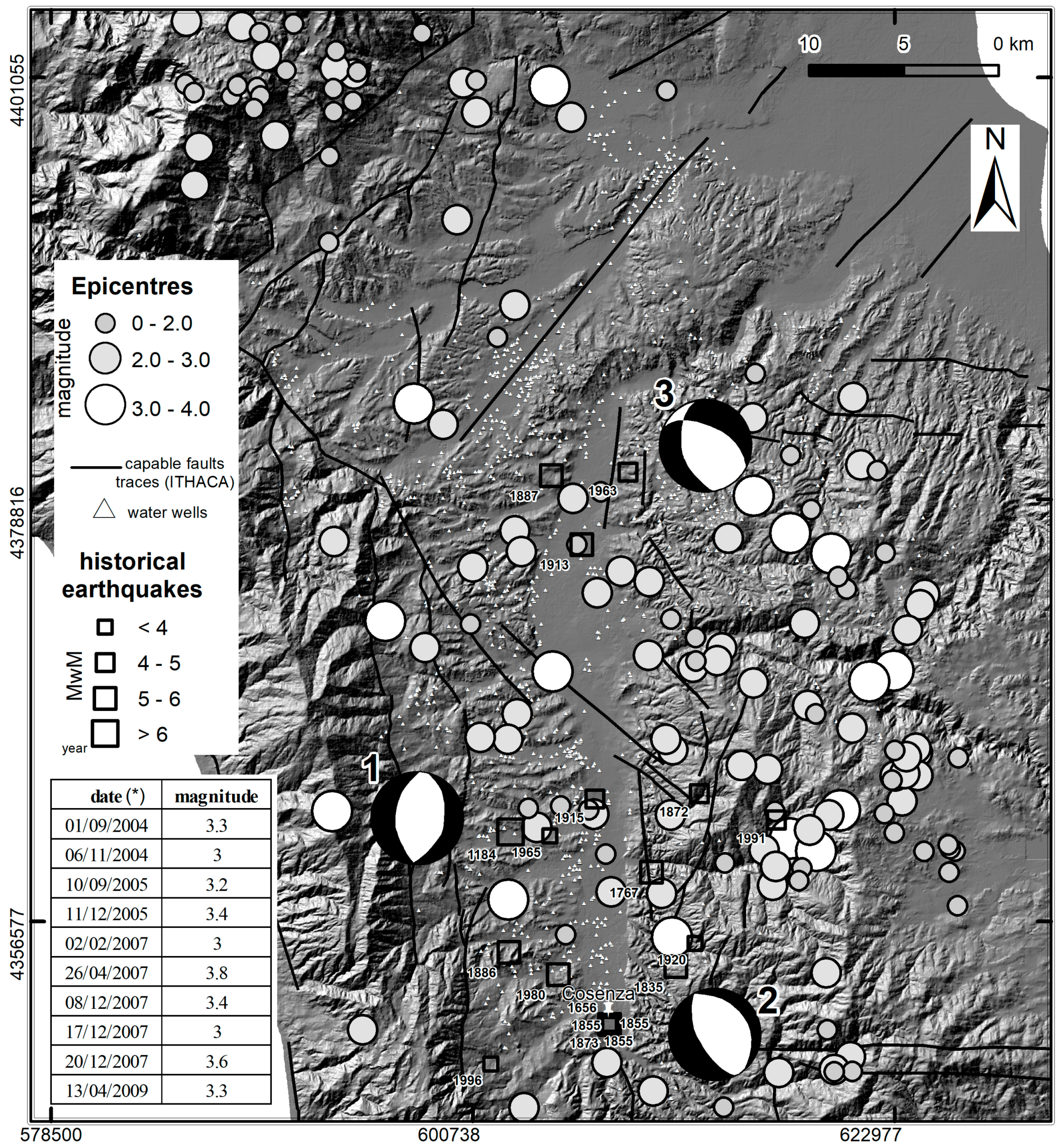
2. Geological Setting
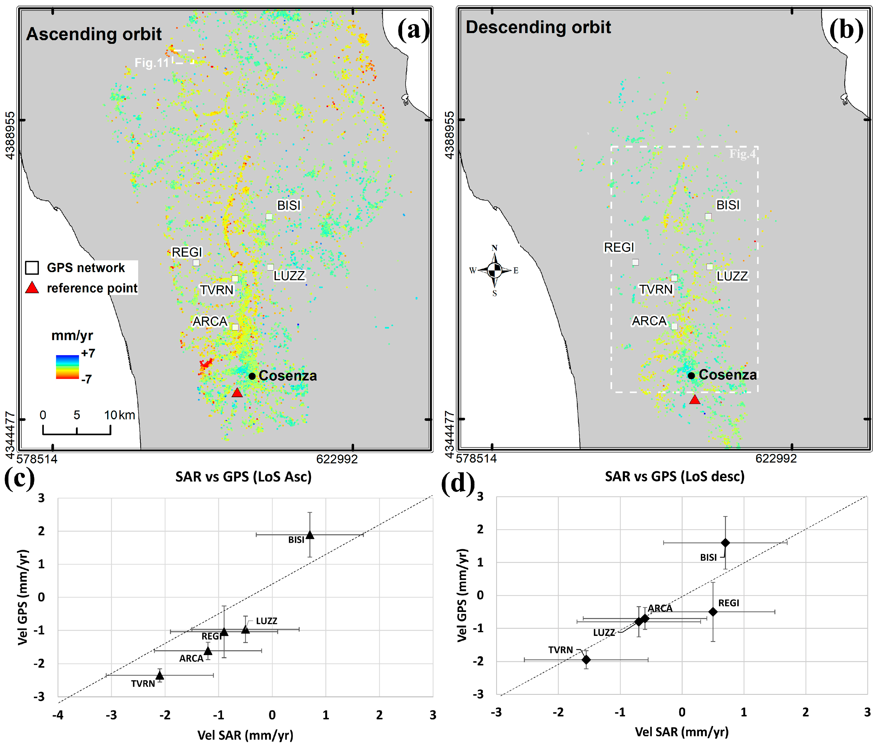
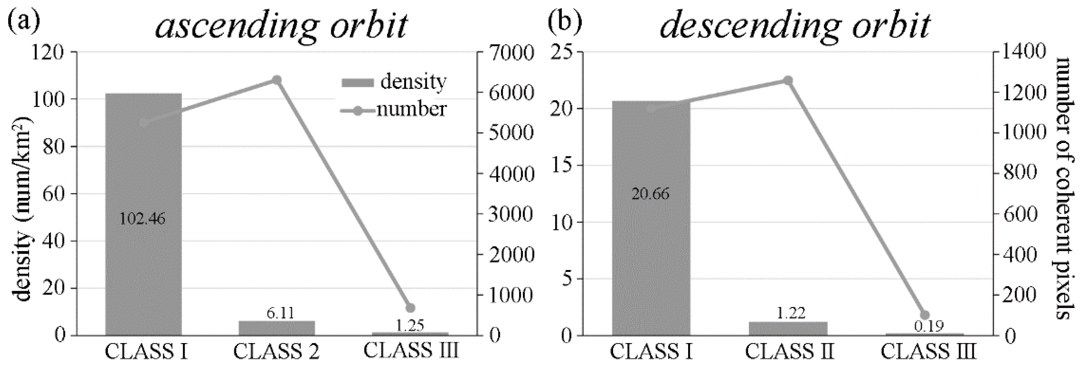
3. Remote Sensing Processing Technique
4. Results
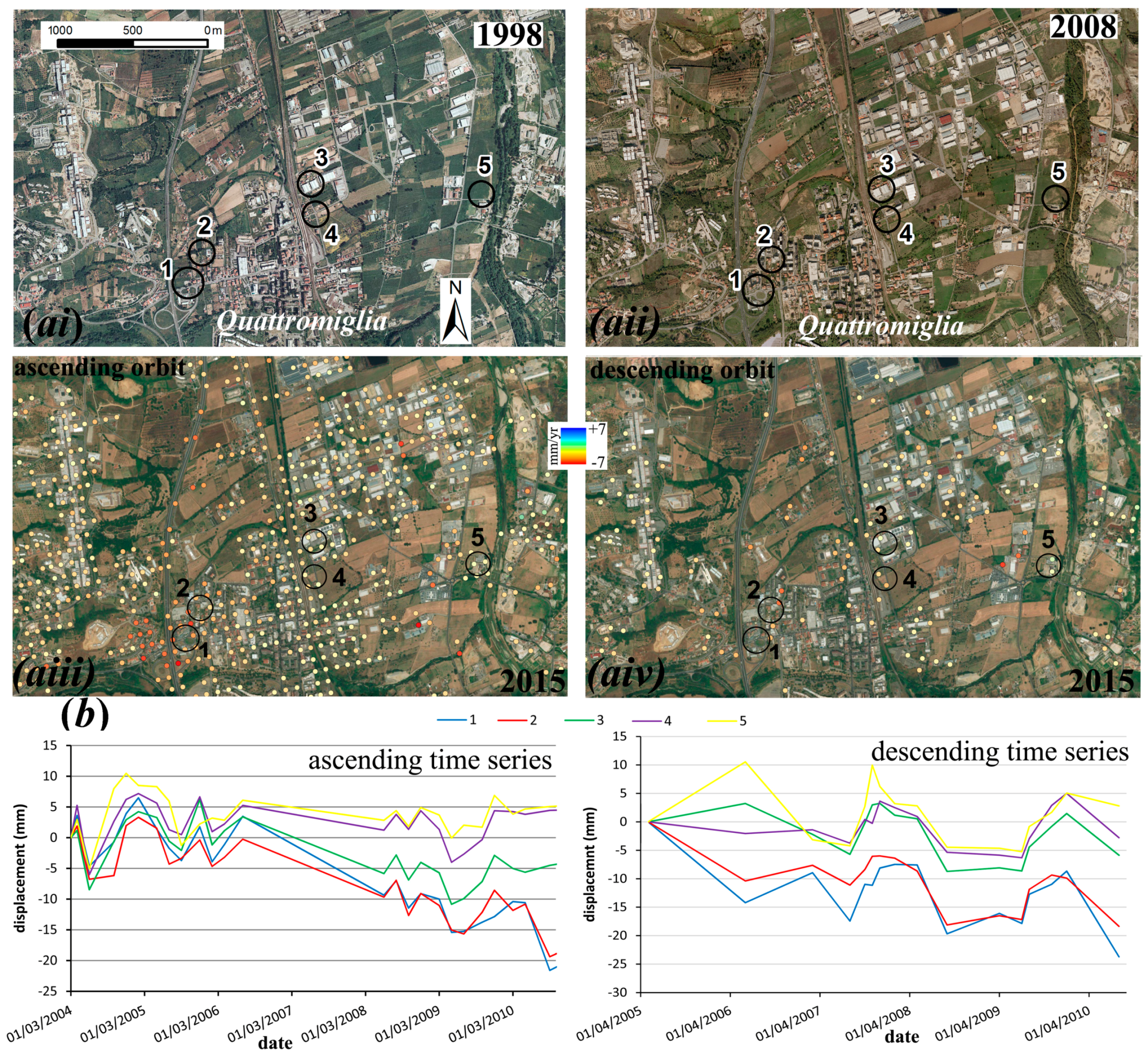
4.1. Alluvial Plain
4.2. Eastern and Western Sides (CV Slopes)
5. Discussion
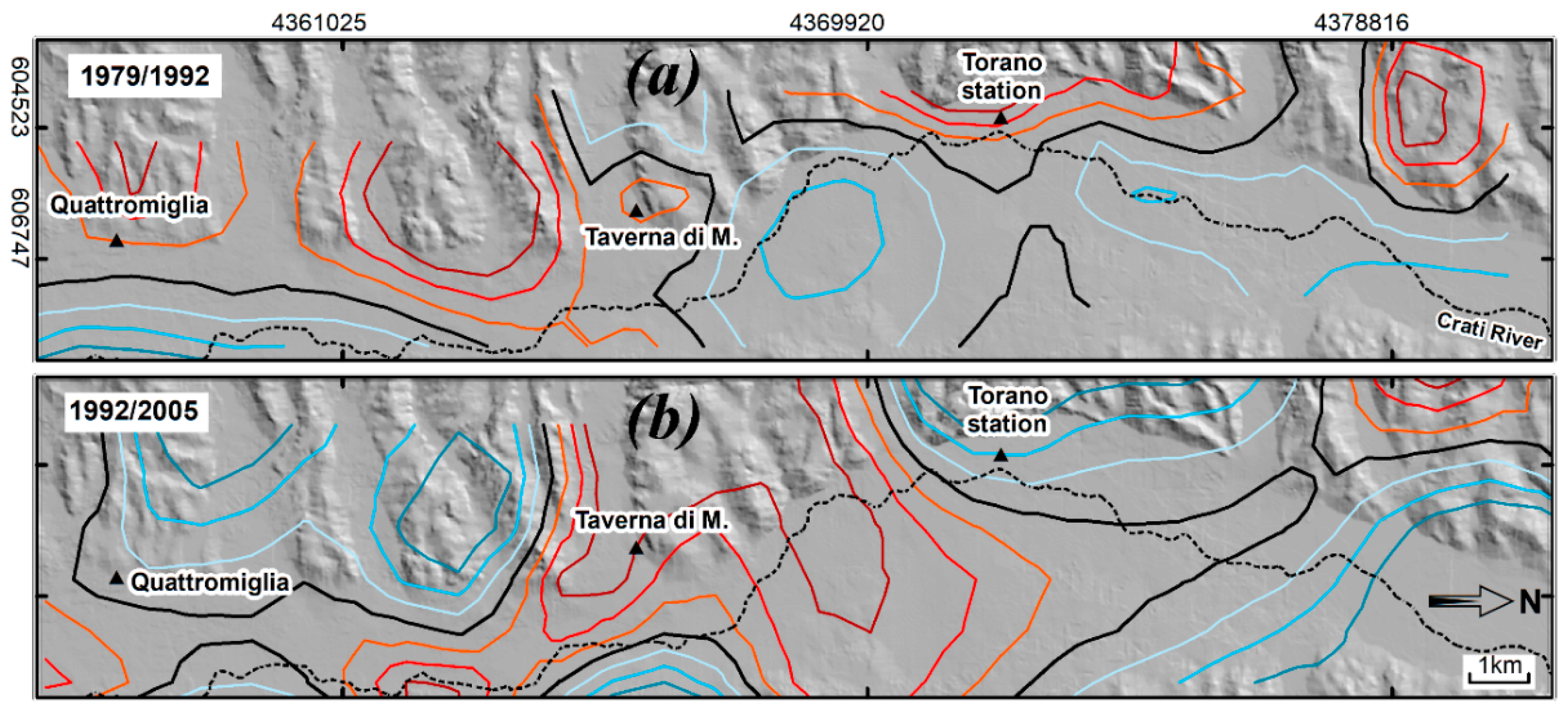
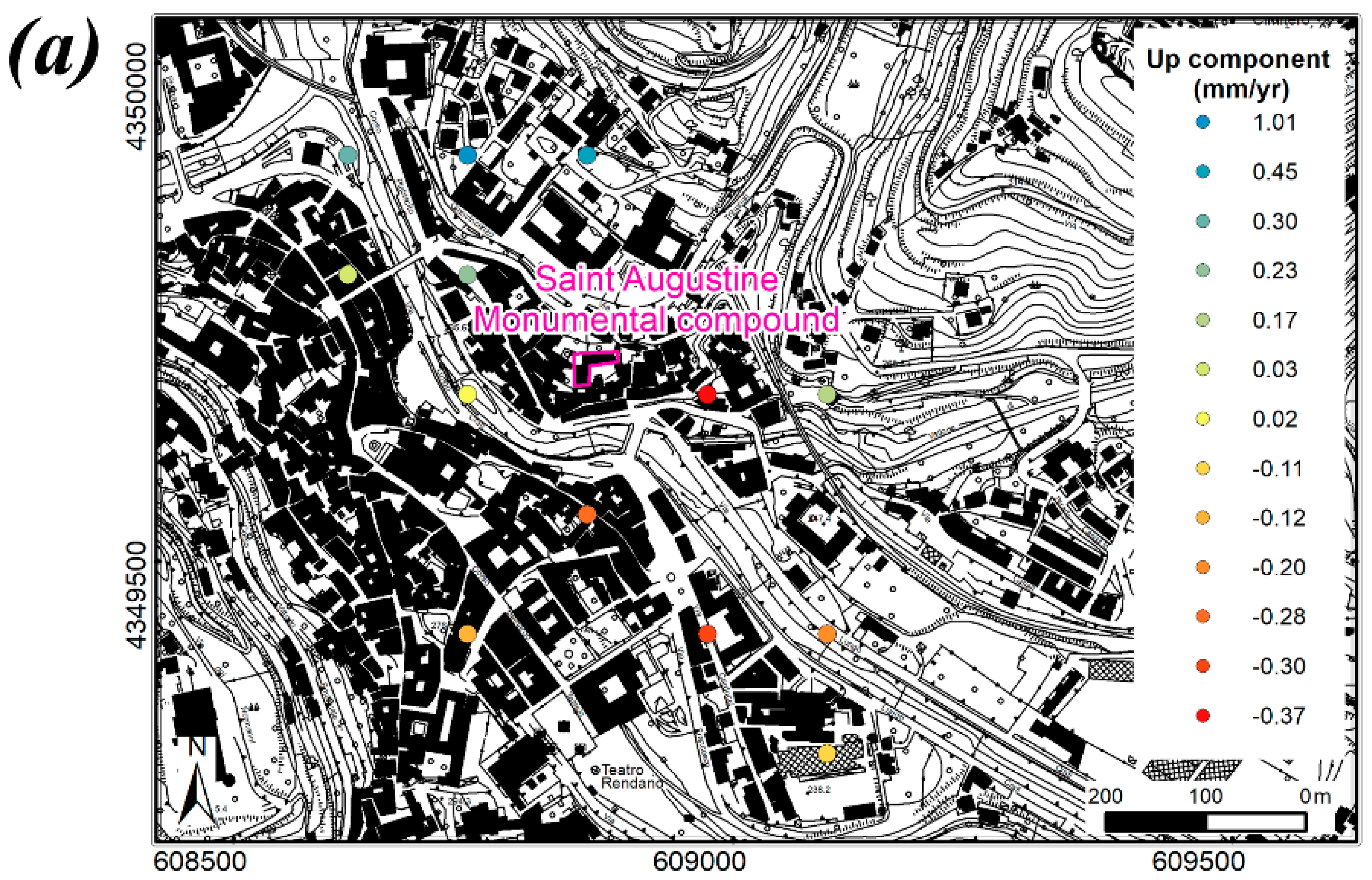
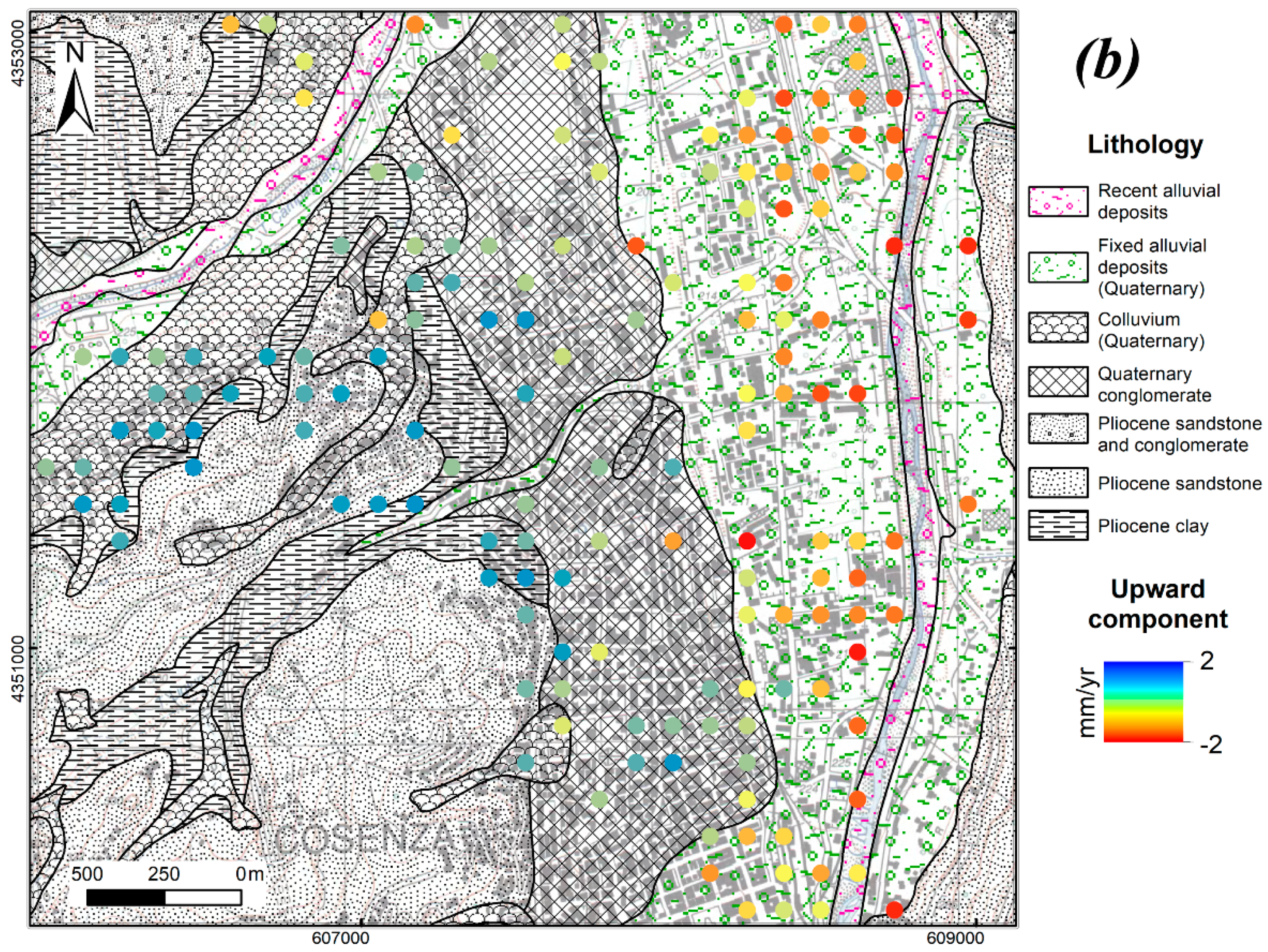
5.1. Subsidence, CV Plain
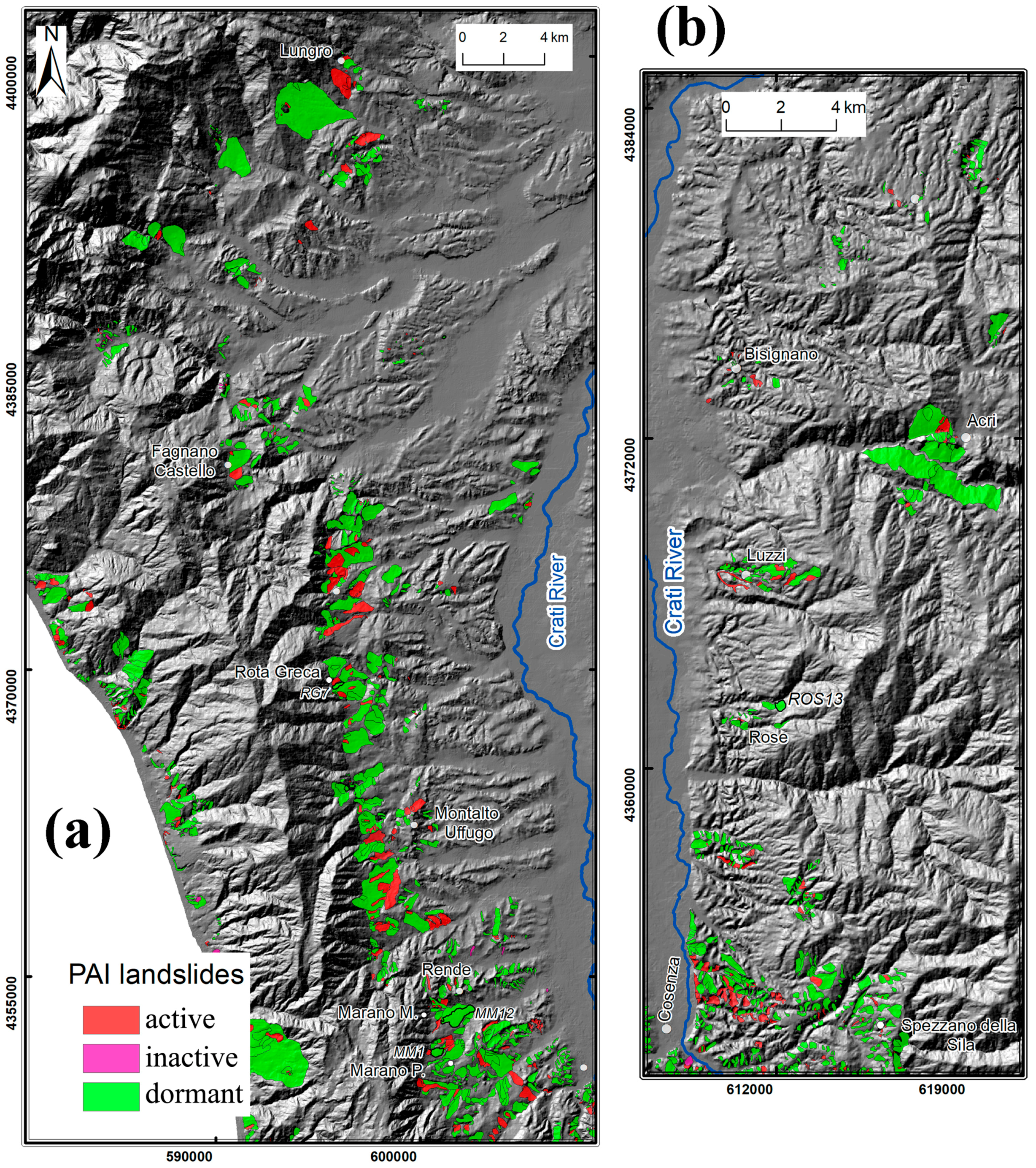
5.2. Landslides, CV Slopes
6. Conclusions
Acknowledgments
Author Contributions
Conflicts of Interest
References
- Gabriel, A.K.; Goldstein, R.M.; Zebker, H.A. Mapping small elevation changes over large areas: Differential radar interferometry. J. Geophys. Res. 1989, 94, 9183–9191. [Google Scholar] [CrossRef]
- Ferretti, A.; Prati, C.; Rocca, F. Permanent Scatters in SAR interferometry. IEEE Trans. Geosci. Remote Sens. 2001, 39, 8–20. [Google Scholar] [CrossRef]
- Berardino, P.; Fornaro, G.; Lanari, R.; Sansosti, E. A new algorithm for surface deformation monitoring based on small baseline differential SAR interferograms. IEEE Trans. Geosci. Remote Sens. 2002, 40, 2375–2383. [Google Scholar] [CrossRef]
- Hooper, A. A multi-temporal InSAR method incorporating both persistent scatterer and small baseline approaches. Geophys. Res. Lett. 2008, 35, L16302. [Google Scholar] [CrossRef]
- Ferretti, A.; Fumagalli, A.; Novalli, F.; Prati, C.; Rocca, F.; Rucci, A. A new algorithm for processing interferometric data-stacks: SqueeSAR. IEEE Trans. Geosci. Remote Sens. 2001, 49, 3460–3470. [Google Scholar] [CrossRef]
- Brunori, C.A.; Bignami, C.; Albano, M.; Zucca, F.; Samsonov, S.; Groppelli, G. Land subsidence, ground fissures and buried faults: InSAR monitoring of Ciudad Guzmán (Jalisco—Mexico). Remote Sens. 2015, 7, 8610–8630. [Google Scholar] [CrossRef]
- Guzzetti, F.; Manunta, M.; Ardizzone, F.; Pepe, A.; Cardinali, M.; Zeni, G.; Reichenbach, P.; Lanari, R. Analysis of ground deformations detected using the SBAS-DInSAR technique in Umbria, Central Italy. Pure Appl. Geophys. 2009, 166, 1425–1459. [Google Scholar] [CrossRef]
- Polcari, M.; Albano, M.; Saroli, M.; Tolomei, C.; Lancia, M.; Moro, M.; Stramondo, S. Subsidence detected by multi-pass differential SAR interferometry in the Cassino plain (Central Italy): Joint effect of geological and anthropogenic factors? Remote Sens. 2014, 6, 9676–9690. [Google Scholar] [CrossRef]
- Stramondo, S.; Saroli, M.; Tolomei, C.; Moro, M.; Doumaz, F.; Pesci, A.; Loddo, F.; Baldi, P.; Boschi, E. Surface movements in Bologna (Po Plain—Italy) detected by multitemporal DInSAR. Remote Sens. Environ. 2007, 110, 304–316. [Google Scholar] [CrossRef]
- Cascini, L.; Fornaro, G.; Peduto, D. Analysis at medium scale of low-resolution DInSAR data in slow-moving landslide-affected areas. ISPRS J. Photogramm. Remote Sens. 2009, 64, 598–611. [Google Scholar] [CrossRef]
- Cascini, L.; Fornaro, G.; Peduto, D. Advanced low- and full-resolution DInSAR map generation for slow-moving landslide analysis at different scales. Eng. Geol. 2010, 112, 29–42. [Google Scholar] [CrossRef]
- Notti, D.; Calò, F.; Cigna, F.; Manunta, M.; Herrera, G.; Berti, M.; Meisina, C.; Tapete, D.; Zucca, F. A user-oriented methodology for DInSAR time series analysis and interpretation: Landslides and subsidence case studies. Pure Appl. Geophys. 2015, 172, 3081–3105. [Google Scholar] [CrossRef]
- Zebker, H.A.; Rosen, P.A.; Goldstein, R.M.; Gabriel, A.; Werner, C.L. On the derivation of coseismic displacement fields using differential radar interferometry: The landers earthquake. J. Geophys. Res. 1994, 99, 19617–19634. [Google Scholar] [CrossRef]
- Moro, M.; Saroli, M.; Tolomei, C.; Salvi, S. Insights on the kinematics of deep-seated gravitational slope deformations along the 1915 Avezzano earthquake fault (Central Italy), from time-series DInSAR. Geomorphology 2009, 112, 261–276. [Google Scholar] [CrossRef]
- Moro, M.; Cannelli, V.; Chini, M.; Bignami, C.; Melini, D.; Stramondo, S.; Saroli, M.; Picchiani, M.; Kyriakopoulos, C.; Brunori, C.A. The October 23, 2011, Van (Turkey) earthquake and its relationship with neighbouring structures. Sci. Rep. 2014, 4, 1–8. [Google Scholar] [CrossRef] [PubMed]
- Jiang, H.; Feng, G.; Wang, T.; Bürgmann, R. Toward full exploitation of coherent and incoherent information in Sentinel-1 TOPS data for retrieving surface displacement: Application to the 2016 Kumamoto (Japan) earthquake. Geophys. Res. Lett. 2017, 44, 1758–1767. [Google Scholar] [CrossRef]
- Brunori, C.A.; Bignami, C.; Stramondo, S.; Bustos, E. 20 years of active deformation on volcano caldera: Joint analysis of InSAR and AInSAR techniques. Int. J. Appl. Earth Obs. Geoinf. 2013, 23, 279–287. [Google Scholar] [CrossRef]
- Spina, V.; Tondi, E.; Galli, P.; Mazzoli, S. Fault propagation in a seismic gap area (northern Calabria, Italy): Implication for seismic hazard. Tectonophysics 2009, 476, 357–369. [Google Scholar] [CrossRef]
- Monaco, C.; Tortorici, L. Active faulting in the Calabrian Arc and eastern Sicily. J. Geodyn. 2000, 29, 407–424. [Google Scholar] [CrossRef]
- Scandone, P. Origin of the Thyrrenian Sea and Calabrian Arc. Boll. Soc. Geol. Ital. 1979, 98, 27–34. [Google Scholar]
- Tortorici, L.; Monaco, C.; Tansi, C.; Cocina, O. Recent and active tectonics in the Calabrian arc (Southern Italy). Tectonophysics 1995, 234, 37–55. [Google Scholar] [CrossRef]
- Mattei, M.; Cipollari, P.; Cosentino, D.; Argentieri, A.; Rossetti, F.; Speranza, F.; Di Bella, L. The Miocene tectono-sedimentary evolution of the Southern Tyrrhenian Sea: Stratigraphy, structural and paleomagnetic data from the onshore Amantea basin (Calabrian Arc, Italy). Basin Res. 2002, 14, 147–168. [Google Scholar] [CrossRef]
- Tansi, C.; Muto, F.; Critelli, S.; Iovine, G. Neogene-Quaternary strike-slipe tectonics in the central Calabrian Arc (southern Italy). J. Geodyn. 2007, 43, 393–414. [Google Scholar] [CrossRef]
- Spina, V.; Tondi, E.; Mazzoli, S. Complex basin development in a wrench-dominated back-arc area: Tectonic evolution of the Crati Basin, Calabria, Italy. J. Geodyn. 2011, 51, 90–109. [Google Scholar] [CrossRef]
- Galli, P.; Bosi, V. Catastrophic 1638 earthquakes in Calabria (southern Italy): New insights from palaeoseismological investigation. J. Geophys. Res. 2004, 108. [Google Scholar] [CrossRef]
- Pondrelli, S.; Salimbeni, S.; Ekström, G.; Morelli, A.; Gasperini, P.; Vannucci, G. The Italian CMT dataset from 1977 to the present. Phys. Earth Planet. Inter. 2006, 159, 286–303. [Google Scholar] [CrossRef]
- Scognamiglio, L.; Tinti, E.; Michelini, A. Real-time determination of seismic moment tensor for the Italian region. Bull. Seismol. Soc. Am. 2009, 99, 2223–2242. [Google Scholar] [CrossRef]
- Mattei, M.; Cifelli, F.; D’Agostino, N. The evolution of the Calabrian Arc: Evidence from paleomagnetic and GPS observations. Earth Planet. Sci. Lett. 2007, 263, 259–274. [Google Scholar] [CrossRef]
- Casula, G. Geodynamics of the Calabrian Arc area (Italy) inferred from a dense GNSS network observations. Geodes. Geodyn. 2016, 7, 76–86. [Google Scholar] [CrossRef]
- Lanzafame, G.; Zuffa, G.G. Geologia e petrografia del Foglio di Bisignano (Bacino del Crati, Calabria): Carta geologica alla scala 1:50000. Geol. Rom. 1976, 15, 223–270. [Google Scholar]
- Di Nocera, S.; Ortolani, F.; Russo, B.; Torre, M. Successioni sedimentarie Messiniane al limite Miocene-Pliocene nella Calabria settentrionale. Boll. Soc. Geol. Ital. 1987, 93, 575–607. [Google Scholar]
- Colella, A.; de Boer, P.L.; Nio, S.D. Sedimentology of a marine intermontane Pleistocene Gilbert-type fan-delta complex in the Crati Basin, Calabria, southern Italy. Sedimentology 1987, 34, 721–736. [Google Scholar] [CrossRef]
- Fabbricatore, D.; Robustelli, G.; Muto, F. Facies analysis and depositional architecture of shelf-type deltas in the Crati Basin (Calabrian Arc, South Italy). Ital. J. Geosci. 2014, 133, 131–148. [Google Scholar] [CrossRef]
- Sorriso-Valvo, M.; Tansi, C. Grandi frane e deformazioni gravitative profonde di versante della Calabria. Note illustrative per la carta al 250.000. Geogr. Fis. Din. Quat. 1996, 19, 395–408. [Google Scholar]
- Tansi, C.; Tallarico, A.; Iovine, G.; Folino Gallo, M.; Falcone, G. Interpretation of radon anomalies in seismotectonic and tectonic-gravitational settings: The south-eastern Crati graben (Northern Calabria, Italy). Tectonophysics 2005, 396, 181–193. [Google Scholar] [CrossRef]
- Tansi, C.; Iovine, G.; Folino Gallo, M. Tettonica attiva e recente, manifestazioni gravitative profonde, lungo il bordo orientale del graben del Fiume Crati (Calabria settentrionale). Boll. Soc. Geol. Ital. 2005, 124, 563–578. [Google Scholar]
- Raspini, F.; Cigna, F.; Moretti, S. Multi-temporal mapping of land subsidence at basin scale exploiting Persistent Scatterer Interferometry: Case study of Gioia Tauro plain (Italy). J. Maps 2012, 8, 514–524. [Google Scholar] [CrossRef]
- Cianflone, G.; Tolomei, C.; Brunori, C.A.; Dominici, R. InSAR time series analysis of natural and anthropogenic coastal plain subsidence: The case of Sibari (Southern Italy). Remote Sens. 2015, 7, 16004–16023. [Google Scholar] [CrossRef]
- Comerci, V.; Blumetti, A.M.; Di Manna, P.; Fiorenza, D.; Guerrieri, L.; Lucarini, M.; Serva, L.; Vittori, E. ITHACA Project and capable faults in the Po Plain (Northern Italy). Ing. Sismica 2013, 30, 36–45. [Google Scholar]
- Rovida, A.; Locati, M.; Camassi, R.; Lolli, B.; Gasperini, P. (Eds.) CPTI15, the 2015 version of the Parametric Catalogue of Italian Earthquakes. Ist. Naz. Geofis. Vulcanol. 2016. [Google Scholar] [CrossRef]
- Massonnet, D.; Feigl, K.L. Radar interferometry and its application to changes in the earth’s surface. Rev. Geophys. 1998, 36, 441–500. [Google Scholar] [CrossRef]
- Bϋrgmann, R.; Rosen, P.A.; Fielding, E.J. Synthetic aperture radar interferometry to measure Earth’s surface topography and its deformation. Annu. Rev. Earth Planet. Sci. 2000, 28, 169–209. [Google Scholar] [CrossRef]
- Hanssen, R. Radar Interferometry: Data Interpretation and Error Analysis; Kluwer Academic Publisher: Dordrecht, The Netherlands, 2001. [Google Scholar]
- Casu, F.; Manzo, M.; Lanari, R. A quantitative assessment of the SBAS algorithm performance for surface deformation retrieval from DInSAR data. Remote Sens. Environ. 2006, 102, 195–210. [Google Scholar] [CrossRef]
- Goldstein, R.M.; Zebker, H.A.; Werner, C.L. Satellite radar interferometry: Two-dimensional phase unwrapping. Radio Sci. 1988, 23, 713–720. [Google Scholar] [CrossRef]
- Pepe, A.; Lanari, R. On the extension of the minimum cost flow algorithm for phase unwrapping of multitemporal differential SAR interferograms. Trans. Geosci. Remote Sens. 2006, 44, 2374–2383. [Google Scholar] [CrossRef]
- De Luca, C.; Cuccu, R.; Elefante, S.; Zinno, I.; Manunta, M.; Casola, V.; Rivolta, G.; Lanari, R.; Casu, F. An on-demand web tool for the unsupervised retrieval of earth’s surface deformation from SAR data: The P-SBAS service within the ESA G-POD environment. Remote Sens. 2015, 7, 15630–15650. [Google Scholar] [CrossRef]
- Farr, T.G.; Kobrick, M. Shuttle Radar Topography Mission produces a wealth of data. Eos 2000, 81, 583–585. [Google Scholar] [CrossRef]
- Celico, F.; De Vita, P.; Monacelli, G.; Scalise, A.R.; Tranfaglia, G. Carta Idrogeologica dell’Italia Meridionale; Istituto Poligrafico e Zecca dello Stato: Rome, Italy, 1999. [Google Scholar]
- Montuori, A.; Luzi, G.; Bignami, C.; Gaudiosi, I.; Stramondo, S.; Crosetto, M.; Buongiorno, F. The interferometric use of radar sensors for the urban monitoring of structural vibrations and surface displacements. IEEE J. Sel. Top. Appl. Earth Obs. Remote Sens. 2016, 9, 3761–3776. [Google Scholar] [CrossRef]
- Almagià, R. Studi Geografici Sulle Frane in Italia: L’Appennino Centrale e Meridionale. Conclusioni Generali; Società Geografica Italiana: Rome, Italy, 1910. [Google Scholar]
- Guerricchio, A.; Bruno, F.; Mastromattei, R. Centri abitati instabili in Calabria: Deformazioni gravitative profonde di versante e grandi frane nel territorio comunale di Lungro (Calabria settentrionale). Geol. Appl. Idrogeol. 1993, 28, 479–488. [Google Scholar]
- Antronico, L.; Borrelli, L.; Peduto, D.; Fornaro, G.; Gullà, G.; Paglia, L.; Zeni, G. Conventional and innovative techniques for the monitoring of displacements in landslide affected area. In Landslide Science and Practice, 2nd ed.; Margottini, C., Canuti, P., Sassa, K., Eds.; Springer: Berlin, Germany, 2013. [Google Scholar]
- Guerricchio, A.; Biamonte, V.; Mastromattei, R.; Ponte, M. Land subsidence induced by slow gravitational deformations and by digging of rock-salt in S. Leonardo territory (Lungro town, Calabria region, Southern Italy). In Proceedings of the 7th Symposium on Land Subsidence, Shanghai, China, 23–28 October 2005. [Google Scholar]
- Cortese, D.; Domestico, G. Lungro Città del Sale; TNT gr@fica: Spezzano Albanese (Cs), Italy, 2010. [Google Scholar]
- Bonì, R.; Herrera, G.; Meisina, C.; Notti, D.; Béjar-Pizarro, M.; Zucca, F.; Gonzàlez, P.J.; Palano, M.; Tomàs, R.; Fernàndez, J.; et al. Twenty-year advanced DIn-SAR analysis of severe land subsidence: The Alto Guadalent´ın Basin (Spain) case study. Eng. Geol. 2015, 198, 40–52. [Google Scholar] [CrossRef]
- Bozzano, F.; Esposito, C.; Franchi, S.; Mazzanti, P.; Perissin, D.; Rocca, A.; Romano, E. Understanding the subsidence process of a quaternary plain by combining geological and hydrogeological modelling with satellite InSAR data: The Acque Albule Plain case study. Remote Sens. Environ. 2015, 168, 219–238. [Google Scholar] [CrossRef]
- Xu, B.; Feng, G.; Li, Z.; Wang, Q.; Wang, C.; Xie, R. Coastal subsidence monitoring associated with land reclamation using the point target based SBAS-InSAR method: A case study of Shenzhen, China. Remote Sens. 2016, 8, 652. [Google Scholar] [CrossRef]
- Perski, Z.; Hanssen, R.; Wojcik, A.; Wojciechowski, T. InSAR analyses of terrain deformation near the Wieliczka Salt Mine, Poland. Eng. Geol. 2009, 106, 58–67. [Google Scholar] [CrossRef]
- Vallone, P.; Giammarinaro, M.S.; Costa, D.; Crosetto, M. Subsidence hazard in potassic salts mines. In Proceedings of the 3rd International Conference on Applied Geophysics for Engineering, Messina, Italy, 11–15 October 2006. [Google Scholar]
- Cetemps. Available online: http://cetemps.aquila.infn.it/chym/valid/index_files/CNR_Calabria_Report.pdf (accessed on 17 January 2017).
- Bianchini, S.; Cigna, F.; Righini, G.; Proietti, C.; Casagli, N. Landslide HotSpot Mapping by means of Persistent Scatterer Interferometry. Environ. Earth Sci. 2012, 67, 1155–1172. [Google Scholar] [CrossRef]
- Bouali, E.H.; Oommen, T.; Escobar-Wolf, R. Mapping of slow landslides on the Palos Verdes Peninsula using the California landslide inventory and persistent scatterer interferometry. Landslides 2017, 1–14. [Google Scholar] [CrossRef]


| Satellite | Orbit Type | Track/Beam | N. of Used Images | Number of Pairs | Temporal Span | Ground Resolution (m) | Incidence Angle (°) |
|---|---|---|---|---|---|---|---|
| Envisat | Ascending | 86 | 26 | 137 | 04/05/2003; 19/09/2010 | 90 | 23 |
| Envisat | Descending | 222 | 17 | 115 | 27/08/2003; 25/08/2010 | 90 | 23 |
| State of Activity | |||
|---|---|---|---|
| Tipology | Active | Dormant | Inactive |
| rotational slides | 83 | 500 | 3 |
| earth flows | 2 | 7 | |
| rock falls | 5 | 1 | |
| deep landslide areas | 49 | 174 | |
| complex landslide | 35 | 102 | 2 |
| surface landslide areas | 23 | 92 | |
| deep-seated gravitational movements | 2 | ||
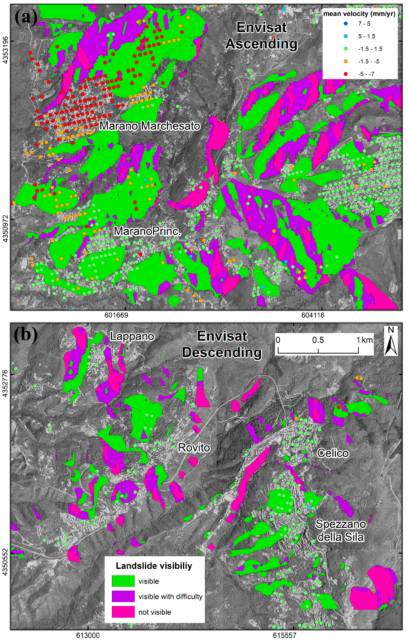
| Visible | Visible with Difficulty | Not Visible | |
|---|---|---|---|
| Descending orbit | areas facing west, northwest, and southwest, and exhibiting slope angles lower than 67° | areas facing north and south | areas facing east, northeast, and southeast |
| Ascending orbit | areas facing east, northeast, and southeast, and exhibiting slope angles lower than 67° | areas facing north and south | areas facing west, northwest, and southwest |
© 2018 by the authors. Licensee MDPI, Basel, Switzerland. This article is an open access article distributed under the terms and conditions of the Creative Commons Attribution (CC BY) license (http://creativecommons.org/licenses/by/4.0/).
Share and Cite
Cianflone, G.; Tolomei, C.; Brunori, C.A.; Monna, S.; Dominici, R. Landslides and Subsidence Assessment in the Crati Valley (Southern Italy) Using InSAR Data. Geosciences 2018, 8, 67. https://doi.org/10.3390/geosciences8020067
Cianflone G, Tolomei C, Brunori CA, Monna S, Dominici R. Landslides and Subsidence Assessment in the Crati Valley (Southern Italy) Using InSAR Data. Geosciences. 2018; 8(2):67. https://doi.org/10.3390/geosciences8020067
Chicago/Turabian StyleCianflone, Giuseppe, Cristiano Tolomei, Carlo Alberto Brunori, Stephen Monna, and Rocco Dominici. 2018. "Landslides and Subsidence Assessment in the Crati Valley (Southern Italy) Using InSAR Data" Geosciences 8, no. 2: 67. https://doi.org/10.3390/geosciences8020067
APA StyleCianflone, G., Tolomei, C., Brunori, C. A., Monna, S., & Dominici, R. (2018). Landslides and Subsidence Assessment in the Crati Valley (Southern Italy) Using InSAR Data. Geosciences, 8(2), 67. https://doi.org/10.3390/geosciences8020067