Ground-Based Remote Sensing and Imaging of Volcanic Gases and Quantitative Determination of Multi-Species Emission Fluxes

Abstract

The physical and chemical structure and the spatial evolution of volcanic plumes are of great interest since they influence the Earth’s atmospheric composition and the climate. Equally important is the monitoring of the abundance and emission patterns of volcanic gases, which gives insight into processes in the Earth’s interior that are difficult to access otherwise. Here, we review spectroscopic approaches (from ultra-violet to thermal infra-red) to determine multi-species emissions and to quantify gas fluxes. Particular attention is given to the emerging field of plume imaging and quantitative image interpretation. Here UV SO₂ cameras paved the way but several other promising techniques are under study and development. We also give a brief summary of a series of initial applications of fast imaging techniques for volcanological research.

1. Introduction

The physical and chemical structure and the spatial evolution of volcanic plumes is of great interest for a number of reasons beyond scientific curiosity:

(A)

Volcanic gas emissions influence the atmosphere and therefore also the climate and other Earth system parameters in a number of ways and on different temporal and spatial scales (e.g., [1,2,3]). Investigations of plume chemistry and plume dispersal will help constrain these influences (see e.g., [4,5]).

(B)

The composition and emission rate of volcanic gases are linked to processes occurring in the Earth’s interior, therefore measuring volcanic gases provides insights into these otherwise largely inaccessible processes. For instance, already Noguchi and Kamiya [6] showed that eruptions of Mt. Asama (Japan) could be forecast with some degree of accuracy by measuring the variable partitioning of sulphur species, chlorine species, and carbon dioxide in the emissions from the active crater. Malinconico [7] showed first that also the amount of gas, in particular the amount of emitted SO₂ varies when the volcanic activity changes. Several authors (e.g., [8,9]) used the measured SO₂ emission also to calculate the amount of magma involved in the simultaneously observed volcanic activity.

These remote sensing techniques have a number of decisive advantages over in-situ observations: The largest being that under most conditions the total amount of gas in the plume can be determined, rather than the gas concentration at the plume edge (usually probed by ground-based in-situ instruments). Since measurements can be made from distances of typically a few kilometres remote sensing is also much safer than in-situ sampling. Moreover, the technology allows easy automation and thus continuous measurements in real time are readily possible, even during periods of explosive activity. In fact continuous measurements of SO₂ and BrO fluxes are realised by the global Network of Observation of Volcanic and Atmospheric Change (NOVAC) [10,11,12].

Recent advances in technology, in particular for spectroscopic techniques, allow remote analysis of many species in volcanic plumes. Specifically, the two-dimensional or even three-dimensional distribution of gases within volcanic plumes and their temporal evolution can now be determined in real time. In other words, recent technology allows “imaging” of trace gas distributions and their motion in plumes. Compared to earlier techniques, which were only capable of measuring the total column density of a particular gas along a single line of sight within the plume (e.g., [13,14,15]), new imaging techniques (see e.g., [5,16]) give much better insight into transport and mixing processes, as well as into chemical transformations within plumes. Moreover, much more accurate, quantitative determinations of trace gas fluxes are now possible in most cases. If the imaging is performed at adequate time resolution, the plume speed can be derived directly from image series, either by correlation techniques (e.g., [13,17,18,19]) or by more advanced image processing techniques (e.g., [20,21,22]).

The most abundant volcanic gases, i.e., H₂O, CO₂, SO₂, HCl, HF, H₂S and many other trace species like BrO, ClO, OClO, NO₂ CO, COS, SiF₄, can be measured either by UV/vis spectroscopy (i.e., H₂O, SO₂, BrO, ClO, OClO, NO₂ are readily measured by DOAS) or IR spectroscopy (e.g., H₂O, CO₂, SO₂, HCl, HF, H₂S, CO, COS, SiF₄). Note, however, that the two species, which are usually most abundant in volcanic plumes (i.e., H₂O and CO₂) also occur in high concentrations in the atmosphere surrounding the plume. Therefore it is frequently difficult to determine these gases by passive spectroscopy (see Section 2.3.3), since the contrast between the background atmospheric signal and background atmosphere plus plume is very small (sometimes in the 10⁻³ range or below).

In the following we give an overview of the principles of optical remote sensing and of plume imaging techniques. These techniques can be applied from the ground, from (manned or unmanned) aircraft (e.g., [23]), or from satellite platforms. Although satellite imaging constitutes an interesting and important branch of these techniques (e.g., [24,25,26]) we restrict ourselves to the first type of application.

At present ground-based remote sensing techniques are in various stages of development, ranging from methods that are already routinely being applied to study volcanic degassing, to those which are so new that only first field test have been done. In addition we discuss applications to flux measurements.

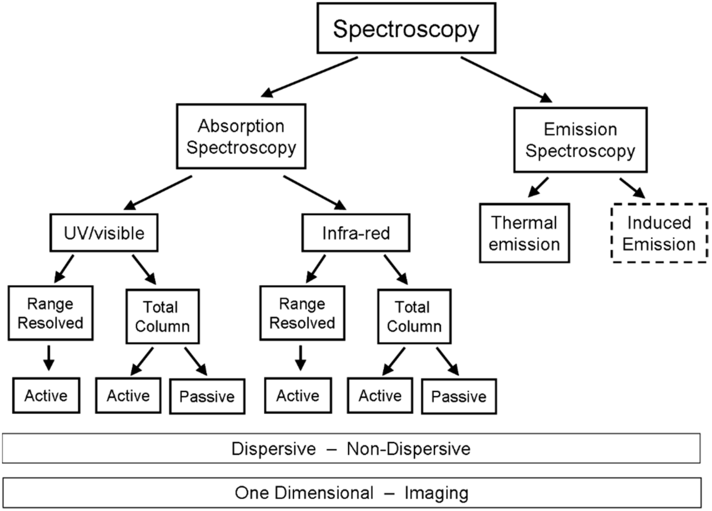
2. Remote Sensing of Volcanic Gases

Remote sensing of volcanic plume composition relies on measuring the absorption, scattering or emission of radiation by the gases (and particulates) in the plume. At this point it is convenient to make a distinction between active (using an artificial light source) and passive (using natural light sources, e.g., the sun or thermal emission) remote sensing. In general, the radiative transfer equation (see e.g., [27]) underlying all these techniques would need to be solved for a remote sensing observer collecting radiation from a certain direction. The remote sensing observer could be located on a satellite in space, on an aircraft or another airborne platform, or on ground. The complexity of the remote sensing problem strongly depends on the chosen vantage point and viewing geometry, the spectral ranges covered, and the abundances of particulates and the target gases in the plume and in the background atmosphere. Figure 1 shows some basic ground based plume sensing schemes.

In the following we give an overview of the principles of optical remote sensing and of plume imaging techniques. We limit ourselves to showcasing ground-based techniques that are regularly used for volcanic plume remote sensing. We recapitulate the basic aspects of absorption (Section 2.1) and thermal emission (Section 2.2) spectroscopic techniques and highlight some applications (Section 2.3). Imaging techniques are discussed in Section 3, below.

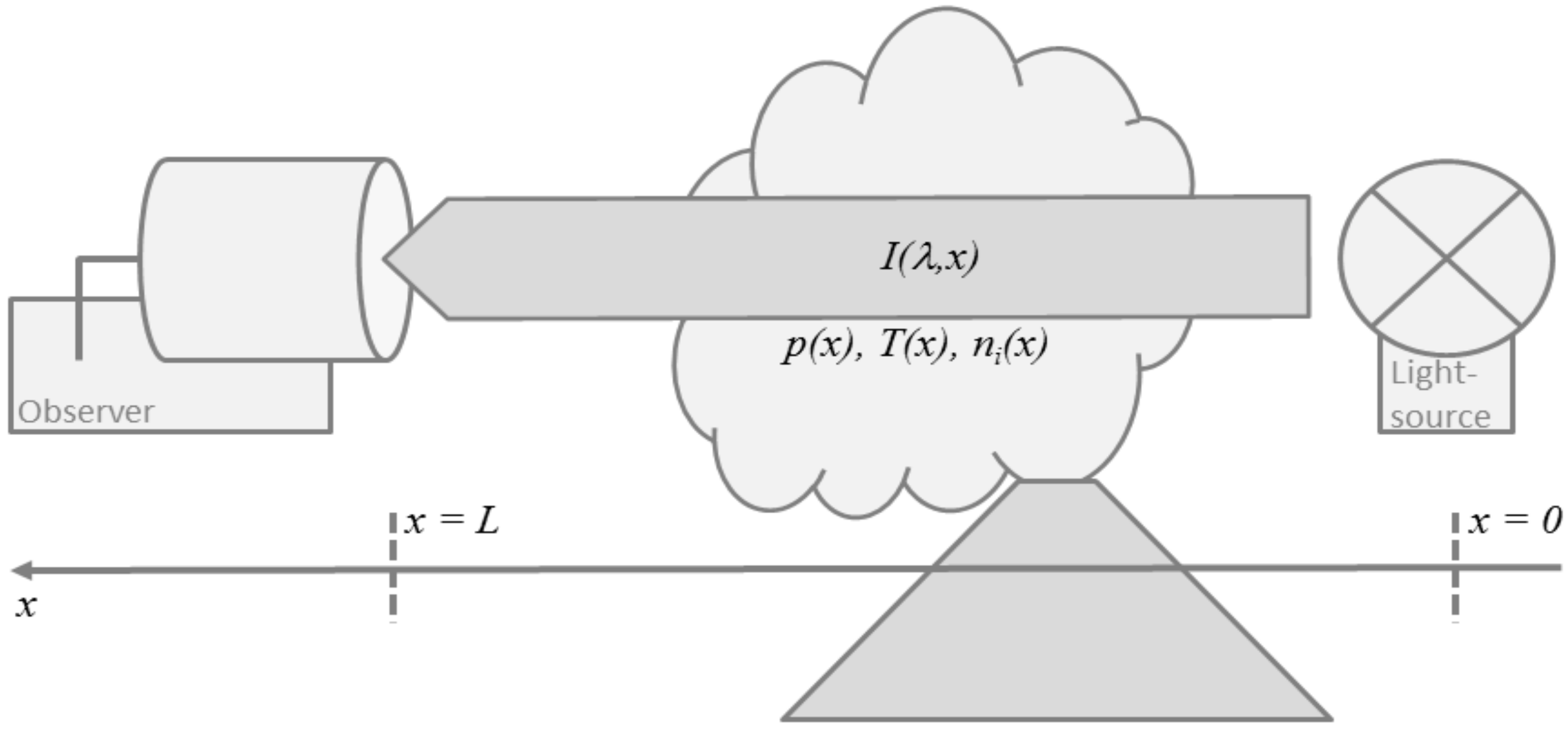
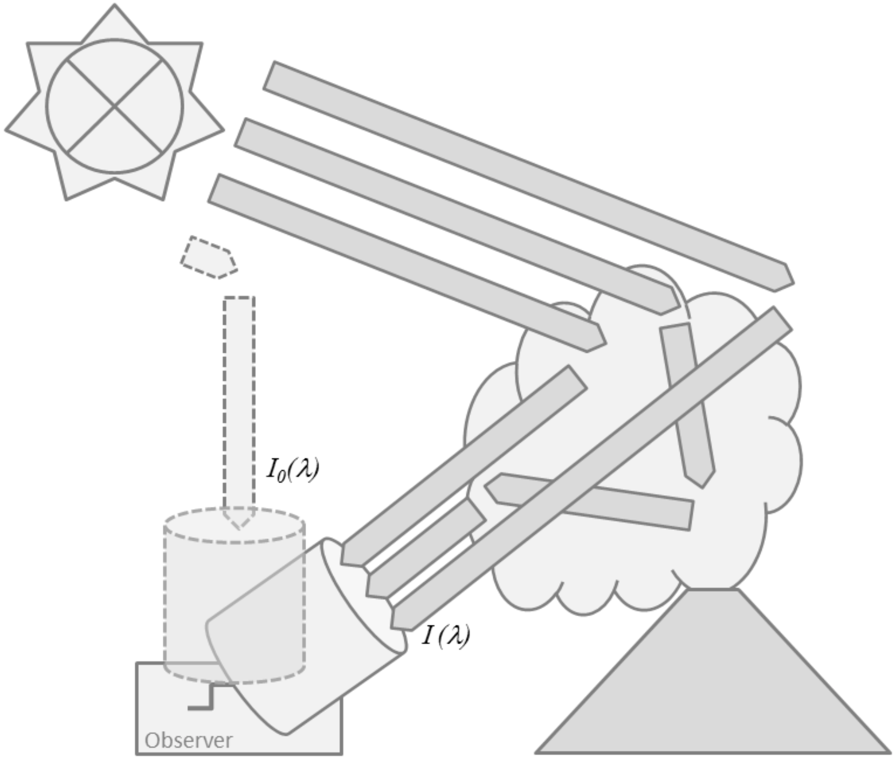
2.1. Absorption Spectroscopy

The classic absorption experiment, illustrated in Figure 2, puts a light source at a distance $L$ from the observer such that the absorbing medium is in-between. Neglecting light-scattering and thermal emission by the medium itself, Beer-Lambert-Bouguer’s law describes the change of the radiance spectrum $I\left(\lambda ,x\right)$ due to absorption along the light path $x$,

$$\frac{dI\left(\lambda ,x\right)}{dx}=-k_a\left(\lambda ,x\right) I\left(\lambda ,x\right)$$

(1)

with wavelength $\lambda$ and absorption coefficient $k_a\left(\lambda ,x\right)$. For a gaseous medium, the latter is given by

$$k_a\left(\lambda ,x\right)={\displaystyle \sum }_i{\sigma }_i\left(\lambda , p\left(x\right), T\left(x\right), \dots \right) n_i\left(x\right)$$

(2)

where $n_i\left(x\right)$ is the number density of absorbing gas species $i$ (of which there might be multiple), and ${\sigma }_i\left(\lambda , p\left(x\right), T\left(x\right), \dots \right)$ is the respective absorption cross section that generally depends on the path via ambient pressure $p$, temperature $T$, or other variables like water vapour that causes spectroscopic effects such as foreign line broadening.

Assuming that the light source emits a background spectrum $I\left(\lambda ,0\right)=I_0\left(\lambda \right)$ at location $x=0$, integration of Equation (1) yields the radiance spectrum at the location $x=L$ of the remote sensing observer,

$$I\left(\lambda , L\right)=I_0\left(\lambda \right)\exp \left(-\tau (\lambda ,0,L\right))$$

(3)

where we define absorption optical density $\tau \left(\lambda ,x_1, x_2\right)$ as

$$\tau \left(\lambda , x_1,x_2\right)={{\displaystyle \int }}_{x_1}^{x_2}{k}_a\left(\lambda ,x\right) dx={{\displaystyle \int }}_{x_1}^{x_2}{\displaystyle \sum }_i{\sigma }_i\left(\lambda , p\left(x\right), T\left(x\right), \dots \right) n_i\left(x\right) dx$$

(4)

If the absorption cross sections can be assumed independent of ambient conditions along the path $\left(p\left(x\right), T\left(x\right), \dots =const.\right)$, the absorption optical density is approximately given by

$$\tau \left(\lambda , 0,L\right)\approx {\displaystyle \sum }_i{\sigma }_i\left(\lambda \right){{\displaystyle \int }}_0^L{n}_i\left(x\right) dx={\displaystyle \sum }_i{\sigma }_i\left(\lambda \right) S_i$$

(5)

where $S_i$ denotes the slant column density of trace gas species i defined as the concentration integrated along the light path. For atmospheric remote sensing, this assumption typically holds for absorption cross sections in the UV and visible spectral range and thus, the Differential Optical Absorption Spectroscopy (DOAS) technique described in Section 2.3.1 adopts Equation (5). In the infra-red, the assumption is not generally applicable and absorption spectroscopic techniques need to start out from Equation (4) (Section 2.3.2), unless the absorbing gases can be safely assumed to only exist in a single plume layer with homogeneous pressure, temperature etc.

Assuming that Equation (5) holds and that there is only a single absorbing gas in the volcanic plume, the respective gas slant column density $S$ can, in principle, be determined by ratioing a background spectrum $I_0\left(\lambda \right)$ by the plume spectrum $I\left(\lambda \right)$ according to,

$$S=\frac{\tau \left(\lambda \right)}{\sigma \left(\lambda \right)}=\frac{1}{\sigma \left(\lambda \right)}\ln \frac{I_0\left(\lambda \right)}{I\left(\lambda \right)}$$

(6)

from which the plume average absorber concentration $\overline{n}$ is straightforward to calculate through

$$\overline{n}=\frac{S}{L_p}$$

(7)

if the species only exists inside the plume (and not in the background atmosphere) and if the geometric path length $L_p$ through the plume can be estimated e.g., using the geometric plume extent. In practice, various complications render this approach too simplistic and real-world solutions need to be found (Section 2.3).

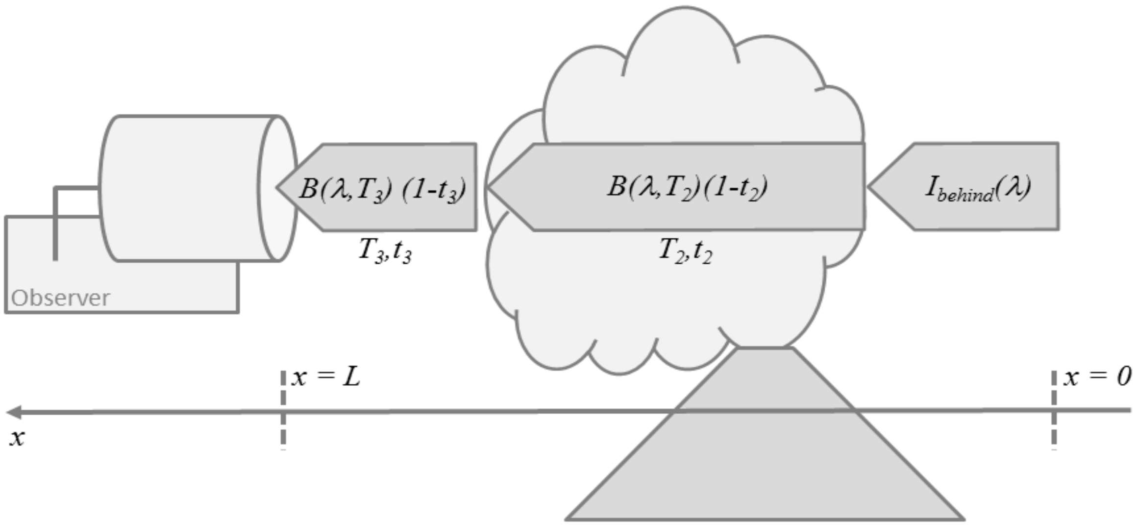
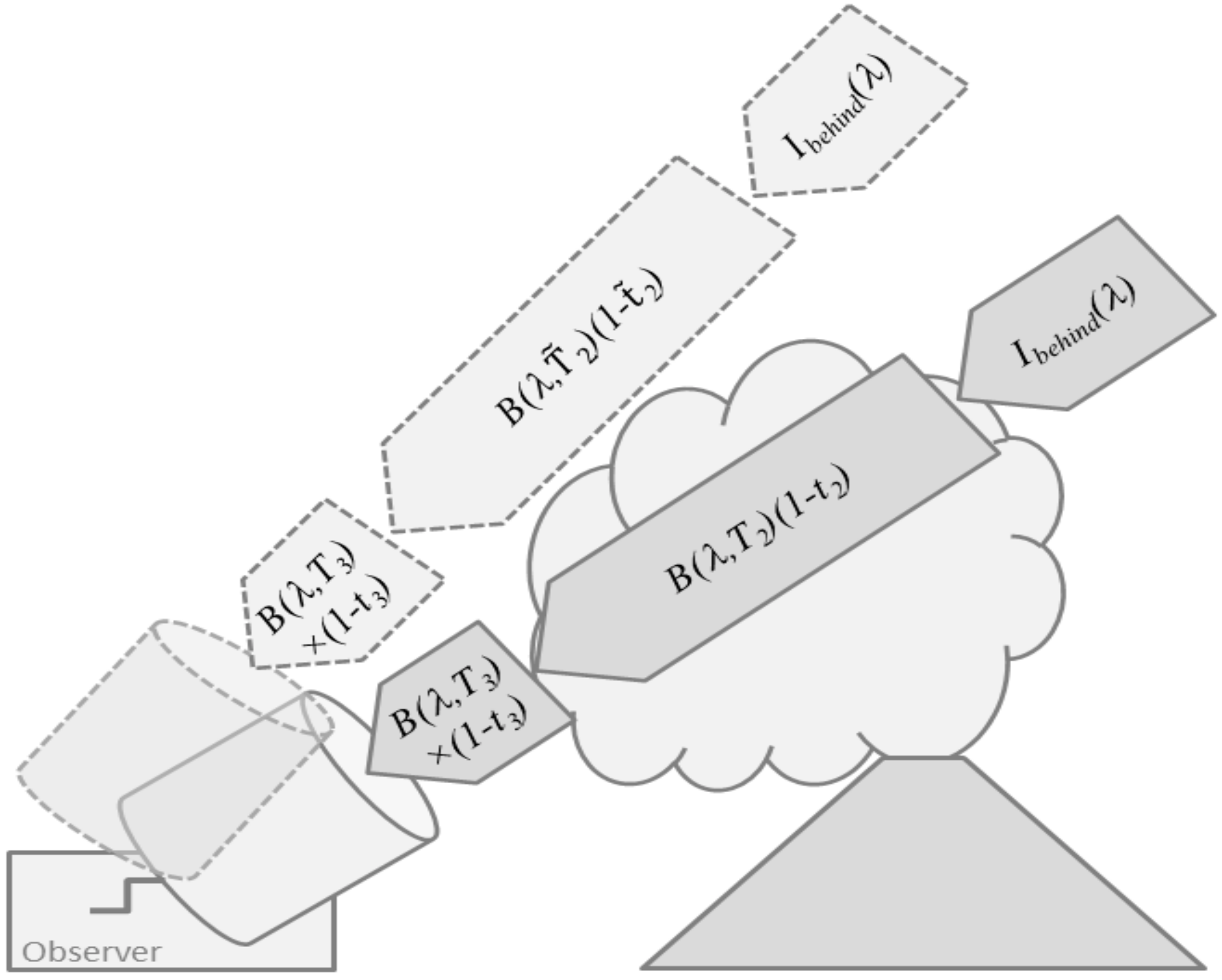
2.2. Thermal Emission Spectroscopy

Thermal emission spectroscopy makes use of the infra-red emission of the atmospheric gases themselves i.e., it collects radiation emitted along the lines-of-sight through the atmosphere in the infra-red spectral range without targeting a specific light source as illustrated by Figure 3. Typically, Schwarzschild’s approximation to the radiative transfer equation is used to describe the emitted radiance spectra,

$$\frac{dI\left(\lambda ,x\right)}{dx}=-k_a\left(\lambda ,x\right) I\left(\lambda ,x\right)+k_a\left(\lambda ,x\right) B\left(\lambda ,T\left(x\right)\right)$$

(8)

where $k_a\left(\lambda ,x\right)$ is the absorption coefficient defined in Equation (2) and $B\left(\lambda ,T\left(x\right)\right)$ is Planck’s thermal emission spectrum

$$B\left(\lambda ,T\left(x\right)\right)=\frac{2 h \frac{c^2}{{\lambda }^5}}{e^{\frac{h c}{\lambda kT\left(x\right)}}-1}$$

(9)

(c = speed of light, h = Planck constant, k = Boltzmann constant, T = temperature). Solving Schwarzschild’s equation for an observer at location $x=L$ pointing toward a cold background at location $=0$ $\left(I(\lambda ,0\right)=0$), with the volcanic plume in-between, yields the observed radiance

$$I\left(\lambda , L\right)={{\displaystyle \int }}_0^L{k}_a\left(\lambda ,x\right) B\left(\lambda ,T\left(x\right)\right)\exp \left(-\tau (\lambda ,x,L\right)) dx$$

(10)

with $\tau (\lambda ,x,L$) the absorption optical density defined in Equation (5). Equation (10) essentially tells that thermal radiation accumulates along the path toward the observer taking into account that radiation emitted at location $x$ gets reabsorbed along the rest of the way to the observer

Dividing the light path into $N$ homogeneous layers $k$ at constant temperature $T_k$ with layer boundaries $x_k$ and $x_{k+1}$, Equation (10) becomes

$$I\left(\lambda , L\right)={\displaystyle \sum }_{k=1}^{N}B\left(\lambda ,T_k\right){{\displaystyle \int }}_{x_k}^{x_{k+1}}{k}_a\left(\lambda ,x\right) \exp \left(-\tau (\lambda ,x,L\right)) dx$$

(11)

which after calculating the integral reduces to

$$I\left(\lambda , L\right)={\displaystyle \sum }_{k=1}^{N}B\left(\lambda ,T_k\right)(1-\exp \left(-\tau (\lambda ,x_k,x_{k+1}\right)) \exp (-\tau \left(\lambda ,x_{k+1},x_{N+1}\right)\left)\right)$$

(12)

Introducing the transmittance $t_k=\exp \left(-\lambda (\lambda ,x_k,x_{k+1}\right)$ of layer $k$ for short-hand notation, Equation (11) reads

$$I\left(\lambda , L\right)={\displaystyle \sum }_{k=1}^{N}B\left(\lambda ,T_k\right) (1-t_k){\displaystyle \prod }_{\begin{array}{c}l=k+1\\ k<N\end{array}}^N{t}_l$$

(13)

A common view on Equation (13) for volcanic applications is the one shown in Figure 3. The emission along the line-of-sight is assumed to consist of three contributions, the atmospheric background radiance $I_{behind}\left(\lambda \right)$ entering the plume from behind, thermal emission by the plume layer (2), and thermal emission by the layer (3) in front of the plume which hosts the observer. Then, Equation (13) simplifies to

$$I\left(\lambda ,L\right)=I_{behind}\left(\lambda \right)t_2{t}_3+ B\left(\lambda ,T_2\right) \left(1-t_2\right)t_3+B\left(\lambda ,T_3\right) \left(1-t_3\right)$$

(14)

Equation (14) carries the target gas concentrations in the plume transmittance $t_2$, and thus can be used to setup plume remote sensing experiments (Section 2.3.3).

For further conceptual insight, we assume that a spectral range can be found where the target gas is the only absorber and that the target gas only exists in the volcanic plume. Then, all layer transmittances except $t_2$ become unity and the background radiance $I_{behind}\left(\lambda \right)$ vanishes, reducing Equation (14) to

$$I\left(\lambda ,L\right)=B\left(\lambda ,T_2\right) \left(1-t_2\right)=B\left(\lambda ,T_2\right) \left(1-\exp \left(-\tau (\lambda ,x_2,x_3\right)\right))$$

(15)

Following the discussion of Equation (5), for a homogeneous plume layer $\left(p\left(x\right), T\left(x\right), \dots =const\right)$, the optical density can be approximated by $\tau \left(\lambda \right)=\sigma \left(\lambda \right)\times S$. Then, Equation (15) readily yields the slant column density $S$ of the target gas via

$$S=\frac{\tau \left(\lambda \right)}{\sigma \left(\lambda \right)}=-\frac{1}{\sigma \left(\lambda \right)}\ln \left(1-\frac{I\left(\lambda ,L\right)}{B\left(\lambda , T_2\right)}\right)$$

(16)

from which the plume average concentration $\overline{n}$ calculates through Equation (7). Thus, under the above approximations, measuring a thermal emission spectrum $I\left(\lambda ,L\right)$ and measuring (or knowing from external sources) the plume layer temperature $T_2$ would allow for estimating the gas concentrations. In practice, infra-red spectral windows are typically packed with overlapping absorption of various background and plume gases and thus, Equation (16) is too simplistic.

2.3. Applications to Remote Sensing of Volcanic Plumes

There is a great variety of ways implement the above theoretical considerations for the purpose of volcanic research and surveillance. The currently available techniques can be broadly grouped into the following categories (see also Figure 4):

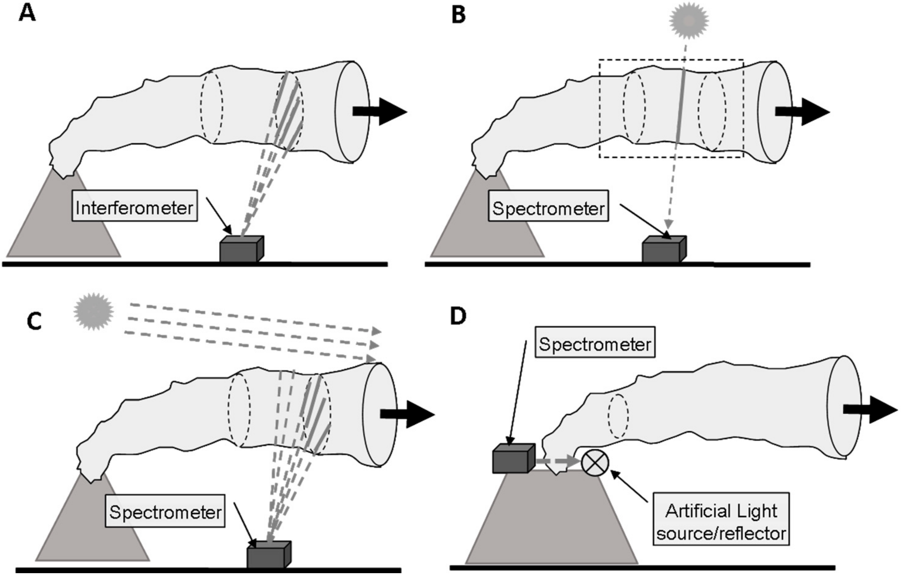
• Active or passive spectroscopy (i.e., will there be an artificial light source or a natural one)
• Arrangement of light path (source-detector, topographic reflector, artificial reflector, backscattered (artificial) light, scattered (sun) light)
• Path integrated column measurement or range resolved detection
• Dispersive or non-dispersive detection

  -

  For dispersive detection: Type of wavelength analysis (grating spectrometer,

  -

  Fourier transform interferometer, Fabry Pérot interferometer, tunable light source, ...)

  -

  For non-dispersive detection: Filter, narrow band emitting light source (e.g., laser, LED)

• One dimensional (single column) or two-dimensional (imaging) measurement (see Section 4)

While there is a large number of possible combinations of the above approaches only several of the techniques have actually been used for remote sensing in volcanological environments and therefore became popular, we describe these in the following:

• Active UV/vis absorption spectroscopy (e.g., DOAS) in Section 2.3.1
• Passive (i.e., scattered sunlight) UV/vis absorption spectroscopy in Section 2.3.1
• IR absorption spectroscopy in Section 2.3.2
• Thermal emission spectroscopy in Section 2.3.3
• LIght Detection And Ranging (LIDAR) in Section 2.3.4

2.3.1. Absorption Spectroscopy in the UV/Visible

Optical absorption spectroscopy (see e.g., [27]) is a technique following the principles outlined in Section 2.1. Absorption cross sections can be assumed to be approximately independent of pressure and temperature in the UV/visible spectral range, and thus, Equation (3) can be combined with Equation (5). However, there is the challenge how to disentangle the minute target gas absorption from overlapping interfering absorption, from spectrally broad extinction of radiation due to light-scattering, and from solar Fraunhofer lines, if the sun is the light source (which is a particularly popular case). Facing these challenges the COSPEC (COrrelation SPECtrometer, e.g., [28]) techniques pioneered UV/vis spectroscopy for volcanic applications from the 1970s. As another approach to address the above challenge, the DOAS (Differential Optical Absorption Spectroscopy) techniques (e.g., [27]) measure absorption spectra in a contiguous range of wavelengths for which the molecular absorption cross sections show several differential structures that are unique fingerprints for the absorbing gases. This implies that absorption cross sections must show strong variations with wavelength to make a gas measurable by DOAS. Today, modern instruments are mostly based on the DOAS technique (e.g., [27]), which our discussions focus on in the following. DOAS can be performed with miniaturized spectrometers and, it is well suited to detect even smallest gas amounts.

Building on the overall idea of using differential absorption structures, DOAS techniques are applicable to direct light-source (sun, moon, or artificial sources, see below) arrangements as well as to applications using scattered (solar) light. In the former case, e.g., when directly pointing into sufficiently bright light sources such as the sun, the path $x$ is the well-defined geometric path between the source and the observer. In the latter case, e.g., when pointing into the sky away from the sun, the path $x$ is the average geometric path that photons travel between the light source and the observer along various individual trajectories such as suggested by Figure 5. This interpretation makes the path $x$, its length $L$ and in consequence the slant column density $S_i$ in Equation (3) depend on wavelength since the average scattering light path depends on atmospheric light-scattering properties such as the particle scattering cross sections and phase functions as well as on the molecular absorption itself, which are all wavelength dependent. However, the narrow spectral ranges and the frequently small absorption optical densities (τ(λ) = 10⁻⁴ … 10⁻¹) encountered in DOAS applications, typically (but not always, see below) allow for dropping wavelength dependencies in $x$, $L$, and $S_i$.

Although solar radiation has considerable intensity in the near IR (up to 2 to 3 µm) typically scattered sunlight absorption spectroscopy is only used in the UV/vis spectral region since it usually relies on Rayleigh scattering, where the scattering efficiency falls off strongly with wavelength (approximately proportional to λ⁻⁴). There is usually also a contribution of Mie (aerosol) scattering, however the intensity of this component also falls off with increasing wavelength (typically proportional to λ^−1.3). A great advantage of using scattered solar light is its universal applicability with observation from only one point, which greatly simplifies the logistics. Dispersive or non-dispersive detectors can be used, up to now the former are employed for one dimensional work and the latter for imaging applications.

Thus, conceptually, DOAS is fit to use Equations (6) and (7) to infer gas concentrations in volcanic plumes. As illustrated by Figure 5, the plume spectra $I\left(\lambda \right)$ in Equation (6) are the measurements for which the lines-of-sight cross the volcanic plume. The background spectra $I_0\left(\lambda \right)$ are obtained by adjusting the observing geometry such that lines-of-sight avoid the volcanic plume or, if such an adjustment is not possible, by resorting to external sources such as solar spectral atlases [29]. In practice, this simple approach faces various complications which need to be overcome.

First and foremost, the absorption optical densities of the target species are typically small (τ(λ) = 10⁻⁴ 10⁻¹) in the UV/visible spectral range and the target absorption usually interferes with strong Fraunhofer lines in the solar spectrum and with absorption by other gases. As explained above, DOAS relies on fingerprinting the target absorption by measuring contiguous spectral ranges covering a sufficient number of differential absorption structures of the target gas. For accessing the minute target absorption with high accuracy, however, it is further crucial to exclude systematic errors originating from uncertainties in the Fraunhofer spectrum or in the absorption cross sections causing spurious effects on the subjacent gas signature. Therefore, DOAS prefers using background spectra (and, if possible, absorption cross sections) that are measured by the actual remote sensing instrument. Then, the aforementioned error sources efficiently cancel, making minute absorption signals accessible.

Strictly, however, Equation (6), assumes the spectra $I_0\left(\lambda \right)$ and $I\left(\lambda \right)$ to be available at an ‘infinite’ spectral resolution i.e., at a spectral resolution much better than the width of the atmospheric spectral features. This is generally not the case when using remote sensing measurements conducted by a field spectrometer. The instrument spectral response function (ISRF) smoothes the atmospheric spectra according to

$$I^{*}\left(\lambda \right)={\displaystyle \int }F\left({\lambda }^{\prime }\right)I\left(\lambda -{\lambda }^{\prime }\right)d{\lambda }^{\prime }=F\left(\lambda \right)\otimes I\left(\lambda \right)$$

(17)

where the symbol $\otimes$ indicates the convolution operation and $F\left(\lambda \right)$ is the ISRF that characterizes the observing instrument. The ISRF can be measured in the laboratory or calculated based on the instrument’s optical and detector properties. Laser based approaches typically have spectrally narrow ISRF and thus, Equation (17) can indeed be dropped. For DOAS applications, replacing $I$, $I_0$, and $\sigma$ in Equation (6) by the measured (or ISRF convolved) quantities $I^{*}$, $I_0^{*}$ and ${\sigma }^{*}$ holds approximately in optically thin conditions. The approximation is applicable for most UV/visible absorbing gases and work-around’s can be found for moderately thick absorption optical densities such that DOAS is widely applicable to trace gas remote sensing in this spectral range.

In practice, DOAS is applied to the retrieval of UV/visible absorbing gases such as H₂O, SO₂, BrO, OClO, NO₂ and O₃ using scattered sunlight as a light source or by directly pointing toward the sun or artificial light sources. In the latter case a broad-band (relative to the absorption band or line) artificial light source, typically in a search light arrangement, supplies a light beam with intensity I₀(λ), which traverses the plume. At the other side of the plume the light is collected and the column density is calculated form the absorption spectrum. Frequently a variant of this set-up is used, where light source and detector are at one end of the light path, while at the other end there is only a reflector (typically a retro-reflector). This arrangement has two advantages: First, the light beam crosses the plume twice, thus doubling the sensitivity and second (and usually more important), all parts of the instrument, which require power are at one end of the light path, while only a passive reflector is at far end. Prerequisite for this approach is the availability of suitable sites on either side of the plume (e.g., two points at the crater rim) for mounting light source and detector or reflector (see e.g., [30,31]). In addition, the technique largely avoids the problems of the large background column density of e.g., H₂O. In principle dispersive or non-dispersive detectors could be used, however, up to now in all applications only the former type is employed.

If the gas under investigation only exists inside the plume and not in the background atmosphere and if scattering effects are not too severe, estimating $n$ from $S$ can be as simple as Equation (7) i.e., dividing the slant column by the length of the line-of-sight transect through the plume. In practice, for measurements using scattered sunlight estimating the intra-plume concentrations from the slant columns $S$ might be complicated due to several effects: (1) the intra-plume average light path has contributions from multiple scattering inside the plume due to large abundances of plume condensate or aerosols, (2) the overall average light path has contributions from photons that do not transect the plume at all and thus, they do not see any target gas absorption (commonly termed light dilution), (3) the target gas has non-negligible abundances in the background atmosphere and thus, background removal is required, or (4) the absorption optical density is not thin and the average scattering light path $x$ cannot be assumed independent of wavelength and the convolution operation does not commute with the exponential in Beer-Lambert-Bouguer’s law.

Following the early introduction of COSPEC (COrrelation SPECtrometer, e.g., [28]), today’s instruments are based on the DOAS technique (e.g., [27]), which can be performed with miniaturized spectrometers. There are also variants with simplified spectral evaluation e.g., Flyspec (e.g., [32]). In principle reflection of sunlight on topographic objects or by clouds could be used, but this has not been attempted yet.

2.3.2. Absorption Spectroscopy in the Infra-Red

In the infra-red (from about 1 to 20 µm wavelength), the absorption cross sections usually depend strongly on pressure and temperature and the absorption optical densities are frequently large, this is particularly true for the thermal IR. Thus, the DOAS approach is not readily applicable. So, generally, Equation (3) in combination with Equations (4) and (17) must be used to forward model the measured absorption spectra based on an initial assumption of gas concentration profiles, plume geometry, and ambient meteorological conditions. An inverse estimation technique iteratively adjusts the target gas concentrations to statistically best match the measurements until some convergence criterion is met.

Absorption spectroscopy in the infra-red mostly relies on direct-light approaches i.e., techniques that have a detector which only accepts radiation from a narrow solid angle centred directly on the light source—be it the sun, a hot telluric source (e.g., lava) or an artificial light source. Thus, Figure 2 is directly applicable. The incoming radiance $I_0\left(\lambda \right)$ in Equation (3) would be the solar Fraunhofer spectrum for direct sun observations, it would be Planck’s thermal emission spectrum $B\left(\lambda , T\right)$, Equation (9), for a hot opaque source with temperature $T$ such as lava, or it would be a silicon carbide lamp (Globar), incandescent lamp, LED (light emitting diode), or laser emission spectrum for artificial light source applications.

As described in Section 2.3.1 direct-light techniques have the great advantage that the light path is well-defined. As long as the light source is sufficiently bright to exclude contributions from light scattering and thermal emission along the atmospheric path, the light path computes easily from the positions of the source and the observer and, if necessary, from the atmosphere’s refractive properties. The major disadvantage of direct-light techniques (as in the case of active UV/vis spectroscopy) is that one has little flexibility in choosing the observing geometry. The line-of-sight is strictly defined by the position of the light source and the receiving system, which have to be arranged such that the volcanic plume is in-between.

IR spectroscopy is implemented in four popular variants:

(a)

With broad-band, thermal light sources, e.g., globars in combination with dispersive detection systems, typically Fourier-Transform interferometers of the Michelson type ([33,34,35]). At volcanoes hot lava can be used as source of radiation (e.g., [36], see below), which—according to our definition—would be classified as passive absorption spectroscopy.

(b)

Tunable Diode laser spectroscopy (TDLS), which (e.g., [37,38,39]) is a variety of dispersive spectroscopy where a narrow-band emitting light source (i.e., a semiconductor laser) is rapidly wavelength modulated in order to sweep across an absorption line of the gas to be measured. The original, rather unreliable lead salt diodes are now replaced by much more stable (though still expensive) quantum cascade laser diodes [40,41]. Since the light source is wavelength modulated there is no need for dispersive detection.

All variants of the technique share the prerequisites (suitable sites) and advantages (low background) with the active UV/vis spectroscopy. Also the options for the arrangement of light paths (single path, retro reflector) are similar, in addition ‘topographic targets’ i.e., back-reflection of the transmitted radiation at terrain surfaces (see below) are in use.

Future developments for active IR spectroscopy could use Dual frequency comb spectroscopy (e.g., [42]), which—although it works differently—has some similarities to a combination of TDLS plus FT spectrometer.

(c)

Passive IR spectroscopy using the sun (or the moon) as a direct light source is commonly referred to as the solar (or lunar) occultation technique which has been used for remote sensing of volcanic gases such as SO₂, HF, HCl, and SiF₄, e.g., [43,44,45]. The technique simplifies substantially if the target gas only exists (at relevant amounts) in the volcanic plume and not in the background atmosphere which is, however, not the case for the major volcanic plume constituents CO₂ and H₂O. Due to the rapid downwind dispersion of the volcanic plume, the volcanic enhancements (on top of the large background) become small and thus, increasingly difficult to measure the farther downwind the plume is sampled. Only recently, Butz et al. [46], demonstrated safe-distance remote sensing of volcanic CO₂ in Mt. Etna’s plume during passive degassing conditions. They operated a sun-viewing, portable Fourier Transform Spectrometer (FTIR) on a truck in stop-and-go patterns underneath Mt. Etna’s plume such that the lines-of-sight to the sun sampled the plume in 5–10 km distance from the crater. Co-measuring O₂ columns helped calibrating spurious variations in the targeted CO₂ columns which were merely due changes in observer position. Sequentially measuring intra-plume and extra-plume spectra and using co-measured HF, HCl and SO₂ as intra-plume tracers helped removing the atmospheric CO₂ background. These current generation instruments were able to discriminate the volcanic CO₂ signal out of a 300-1000 times larger atmospheric background path.

(d)

Hot volcanic material such as lava or volcanic rocks have been used heavily in open-path spectroscopic techniques, e.g., [33,35,36,43,47,48,49,50,51] Naughton et al. 1969, Mori et al. 1993, Notsu et al. 1993, Mori et al. 1995, Francis et al. 1998, Mori and Notsu, 1997, Burton et al. 2000, Gerlach et al. 2002, Allard et al. 2005] targeting volcanic SO₂, HF, HCl, SiF₄, CO, CO₂, COS. Generally, the technique requires that the hot material or the lamp locates behind the plume and that it can be sighted by the observer. For many volcanoes, this requirement implies deploying instrumentation in the proximity of the crater or at the crater rim which spoils the general remote sensing advantage of avoiding hazards and hostile environments to operators and instrumentation. Recently, laser-based techniques for CO₂ have been developed using topographic reflection targets, e.g., [52,53], promising greater deployment flexibility but still requiring plume sampling close to the source where CO₂ enhancements are large compared to the atmospheric background.

2.3.3. Thermal Emission Spectroscopic Techniques

Typically, Equation (14) forms the basis for volcanic plume remote sensing by thermal emission spectroscopy, e.g., [54,55]. Using a forward modelling approach similar to the one used for direct-light absorption spectroscopic techniques, one starts out with an initial guess for the ambient and plume temperatures as well as for the transmittances. The transmittances contain the layer-wise optical densities and thus, the information on the layer-wise gas composition. Iteratively, the targeted plume gas abundances are adjusted to yield a best match of measured and forward modelled spectra.

Thermal emission spectroscopy allows for the detection of other species than UV/vis absorption spectroscopy (see Section 2.3.1) and for observation independent of sunlight, i.e., also at night time.

Disadvantages include complicated set-up (FT-IR), usually cryogenic cooling of the detector is required. However recently also non-dispersive detection with detectors at room temperature was demonstrated [56,57]. The classic approach is the differential one sketched in Figure 6, using the difference between two measurements, one pointing into the plume and one pointing next to the plume into the background sky, e.g., [54,58]. For these two measurements, the recorded measurements approximately differ by temperature $T_2$ and transmittance $t_2$ in Equation (14) either referring to intra-plume or background conditions. Thus, the difference spectra isolate the information on the targeted plume composition which is straightforward to retrieve as outlined in Goff et al. [54], Stremme et al. [55], and Krueger et al. (2013) [59], used a thermal emission FTIR to sequentially scan the SO₂ and SiF₄ plume (and the adjacent background sky) of Popocatepetl volcano from 12 km distance providing a series of two-dimensional images of the volcanic gas columns. Then, they used the series of images to simultaneously estimate the plume average wind speed and the constituent outflux from the crater. Current developments toward imaging FTIRs (e.g., [57,60]) are promising for use in volcano plume monitoring since they allow for rapidly imaging the thermal emission spectrum emerging from two-dimensional scenes without the need for scanning a telescope.

2.3.4. Range Resolved (LIDAR) Techniques

A further, well known approach to active remote sensing trace gases is the LIght Detection and Ranging (LIDAR) technique, e.g., [61,62]. The usual set-up is the mono-static LIDAR where transmitter and receiving system are at the same location. The (laser) light source emits short (<few 100 ns) pulses into the atmosphere. By analyzing the time profile of the intensity back-scattered from the atmosphere the spatial distribution of scattering and extinction along the direction of the emitted (and received) radiation can be deduced. With single-wavelength lasers aerosol backscatter and extinction are measured.

In order to determine trace gas distributions a more complicated set-up is required. These devices have become known as Differential Absorption Lidar (DIAL) using at least two wavelengths, one “on absorption” of the trace gas and one “off absorption” [13,14,63,64]. The approach is similar to the SO₂-camera (see Section 3.2.1). While DIAL systems have been bulky, relatively complicated and power consuming recent developments including micro-pulse diode lasers (e.g., [65]) promise smaller, lower power, and more portable systems.

Alternatively to the customary mono-static approach a bi-static LIDAR scheme has been developed (e.g., [4,66,67]). Here, radiation source and radiation detector are separated by a small distance (on the order of 10 m for a few km range) and the range resolution is accomplished by changing the elevation angle of either the radiation source or of the radiation detector. Advantages are the possibility to use continuous light sources (like LEDs) and simpler detection.

In principle two-dimensional or even three-dimensional push-broom imaging of volcanic plumes is possible with LIDAR instruments and to some extent has been demonstrated at volcanic plumes (e.g., [13,14,63]).

3. Imaging of Plumes

Many of the developments for volcanic plume remote sensing have started with collecting a series of individual plume (column density) measurements in order to sample one-dimensional plume cross sections. Modern technology allows to ‘image’ plumes, i.e., to provide two-dimensional arrays of optical densities (or ‘images’) of a scene containing volcanic gases. This approach offers many advantages over the simpler one-dimensional plume scanning:

• Complex situations (multiple plumes, change of wind direction, etc.) can be recognised and analyzed (e.g., [68])
• Advanced techniques of image analysis (e.g., segmentation and optical flow analysis) can be applied, thus enabling more precise flux determination (e.g., [22,69,70]), see also Section 4, below.
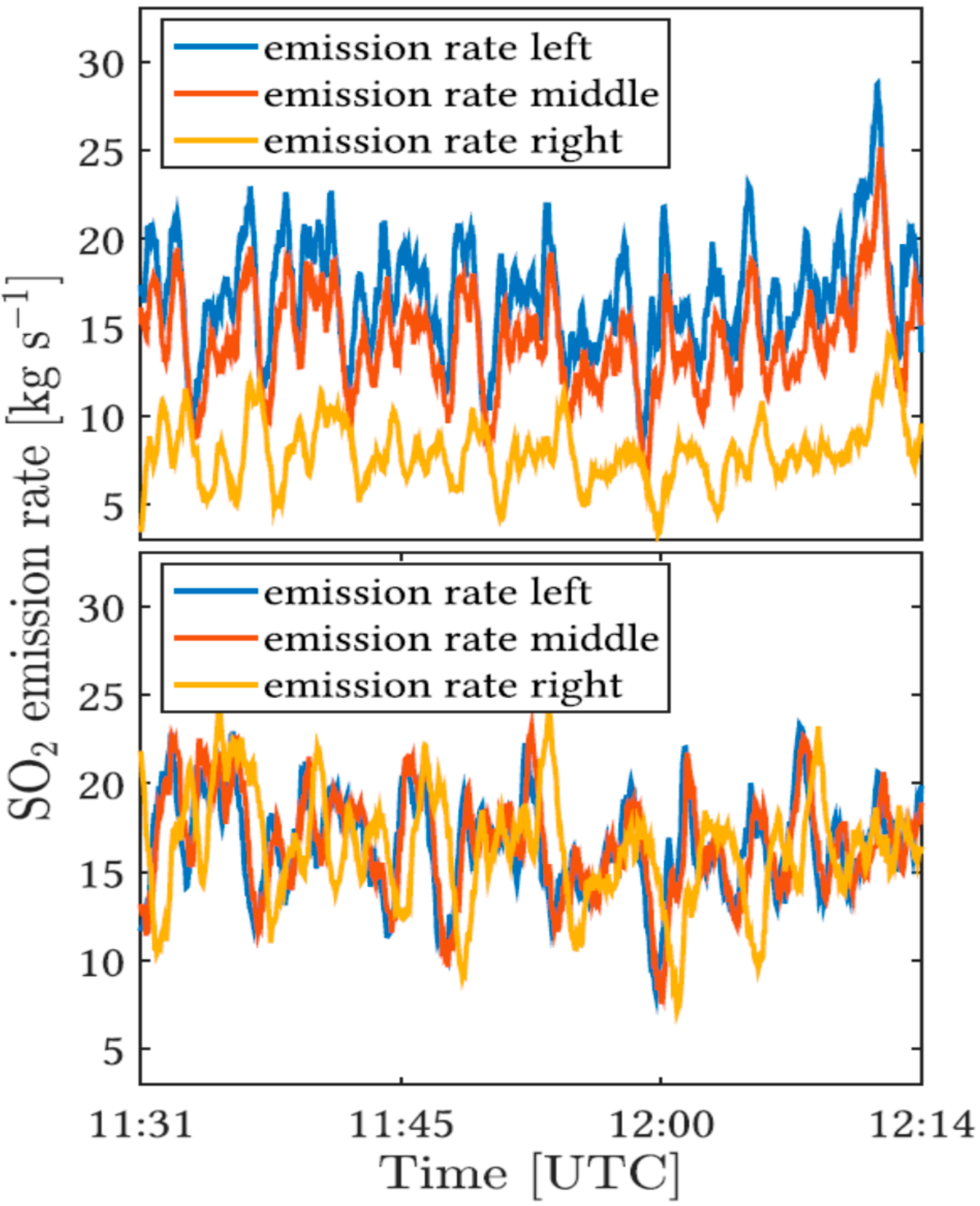
• Redundant measurements can be made by e.g., making trace gas flux determinations at several planes along the plume propagation direction allowing e.g., internal consistency checks (see e.g., [22])
• Redundant flux measurements can be used to determine the exact plume propagation direction (see [22])
• Last not least: the human visual system has powerful analysis capacities which can be used once images are available (‘seeing is believing’)

For these (and more) reasons a series of imaging systems for volcanic plumes have been developed and applied (see e.g., [5,16]). In this context the requirements for plume imaging instruments include:

• Capability to specifically detect the desired gas (or parameter)
• To provide sufficient sensitivity (e.g., for SO₂ measurements a detection limit for SO₂-column densities of the order of 10¹⁷ molecules/cm² or ca. 40 ppmm is required for volcanic emissions observations)
• To provide sufficient spatial resolution to allow discrimination of the relevant features within the plume(s)
• Sufficient time resolution (typically of the order of seconds) of the measurement is further required to be able to resolve the motion of the plume and variations in the volcanic source strength

Some of these requirements are in conflict with each other. For example enhanced specificity may be achieved by recording of the intensity at several wavelengths, since this typically can only be done sequentially the time resolution will be reduced. Likewise, lower detection limits (i.e., higher sensitivity) are achieved by collecting a larger number of photons per pixel, which comes at the expense of time resolution (or, alternatively, spatial resolution). In particular, the number of gases which can be detected by imaging instruments is limited in comparison to one dimensional instruments.

It should be noted that there is a connection between spatial and temporal resolution in that a given spatial resolution requires sufficient temporal resolution to be useful. The motion of the plume ∆x = v·∆t within the acquisition time ∆t of an image (v = wind speed) should be at least of the order of the size of one picture element in the plane of the plume. In other words, high spatial resolution makes sense only if the technique also offers sufficient temporal resolution (for a given wind speed). Note that the opposite is not necessarily true: A temporal resolution exceeding the above limit would still result in useful (though partly oversampled) data.

As described in Section 2 several remote sensing techniques for the imaging of plumes have been developed during recent years. As described in Section 2.3.2 and Section 2.3.3 the various techniques can be grouped into active and passive as well as in dispersive and non-dispersive approaches. For dispersive approaches several scanning schemes are possible as detailed in Section 3.1, below.

The characteristics of dispersive techniques is the determination of a spectrum (i.e., a series of intensities as function of wavelength) for each pixel of the image. The trace gas column density for each pixel is then derived from the measured spectrum using the algorithms described in Section 2, above. Non-dispersive approaches, on the other hand, derive the column density from the ratio of just a few (typically two) intensity measurements integrated over suitable (narrow) wavelength intervals. Frequently, a reference intensity ratio is recorded with the instrument pointed away from the plume. The trace gas column densities are then derived from the ratio of the sample and reference intensity ratios.

Dispersive approaches include variations of Differential Optical Absorption Spectroscopy (DOAS, see Section 2.3.1, above, and e.g., [27]) and Fourier-Transform Infra-red (FTIR) spectroscopy (e.g., [47]) adapted to allow two-dimensional measurements.

Dispersive approaches are typically more complex and since usually scanning is required slower than non-dispersive techniques. However, they have the advantage of being less vulnerable to spectroscopic interferences and to be able to also measure minor constituents like BrO due to higher spectral resolution enabling higher specificity for gas detection. Furthermore, analysis using traceable, well quantified absorption cross-sections increases the rigour of the technique. Many gas absorption features are naturally narrow (of the order of 1–2 nm), particularly for small molecules, and this limits the effectiveness (i.e., the sensitivity as well as the capability to specifically detect a particular species) of non-dispersive techniques.

Note that any combination of dispersive/non-dispersive techniques is in principle possible and several combinations have been realized, such as the combined use of a dispersive UV spectrometer alongside a non-dispersive UV imaging system (see e.g., [71]). In fact, an important aim of present research is the development of techniques combining the speed of non-dispersive techniques with the rigor of dispersive techniques. Overall, despite impressive accomplishments, techniques for quantitative imaging of volcanic plumes are still in an early stage of development and much progress can be expected in the near future.

3.1. Categories of Plume Imaging

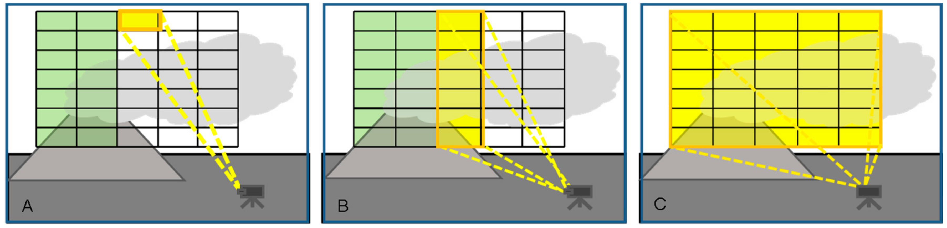
Two dimensional images of trace gas column amounts are derived from three-dimensional data: two spatial dimensions and one wavelength (or interferogram) dimension are recorded. At present three different imaging techniques are known (see Figure 7 and

Table 1. Characteristics of the three basic imaging techniques.

Imaging Principle	Detector Type	Examples/Comments
Whisk-broom	Spectrometer or Michelson Interferometer	Experimental instruments [55]
	Filter	not used
	Fabry-Pérot Interferometer	Theoretical studies, [79,80]
	Gas Correlation	Presently not used
Push-broom	Spectrometer	I-DOAS, [74], Imaging Sagnac-Interferometer [57] FTIR
	Filter	Presently not used A
	Fabry-Pérot Interferometer	Presently not used A
	Gas Correlation	Presently not used A
Full-Frame	Wavelength sensitive pixels	Future Technology (e.g., [81])
	Filter	UV SO2-camera e.g., [19,82] and references in the text
	Fabry-Pérot Interferometer	Theoretical studies in the UV [79], in use in the IR [60]
	Gas correlation	Presently not used A

^A For volcanic plume imaging.

):

(1)

Pixel at a time scanning (“whiskbroom” imaging, see Figure 7A): In this approach all pixels of an image scene are scanned sequentially according to a particular scheme (e.g., line by line as in early TV cameras), for each pixel a spectrum is determined. In this approach all (of e.g., 10⁵ pixels) have to be scanned individually, such that it is potentially a rather slow approach. Michelson interferometers have been combined with whisk-broom scanners to obtain 2-D images (e.g., [34,55,72]).

(2)

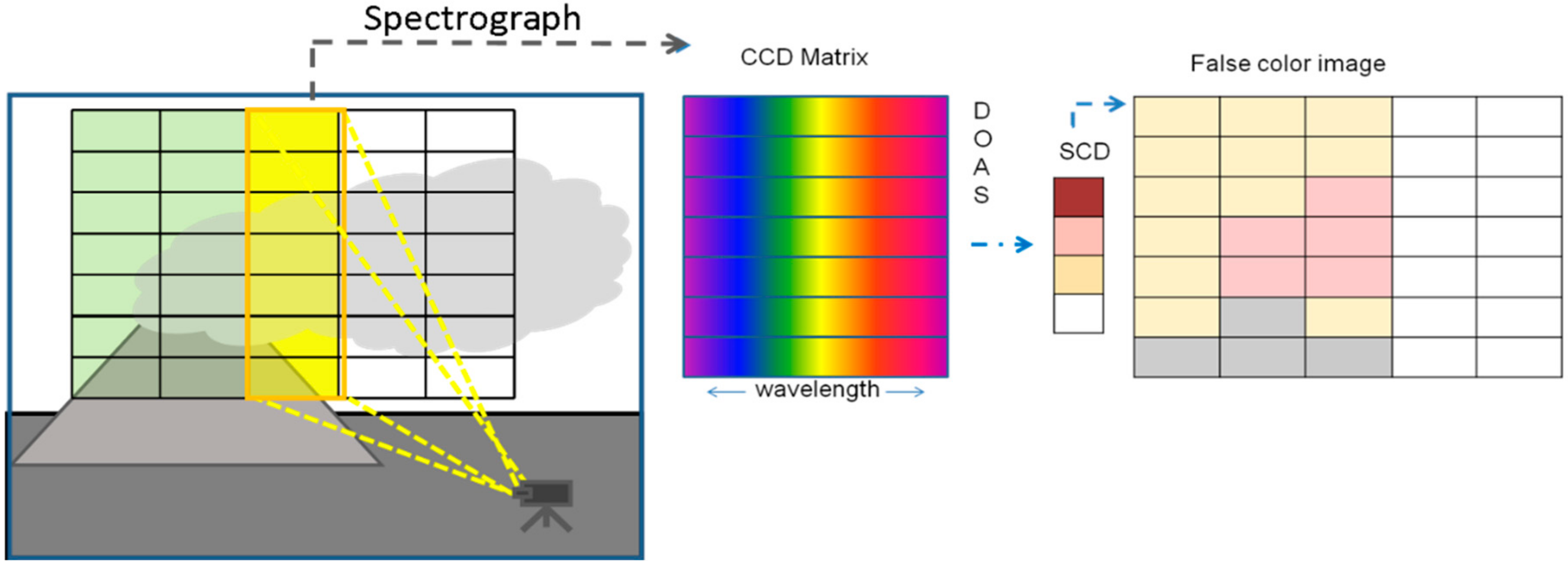
Column (or row) at a time scanning (“push-broom” imaging, see Figure 7B): Here all pixels of an image column are scanned simultaneously while the image columns are scanned sequentially. Because each column of the image is recorded at once, only of the order of several hundred columns have to be measured sequentially. Since only one scan-dimension is required the scanning mechanisms can become simpler though it is not necessarily faster. In fact, as will be explained below the amount of radiation collected by the entrance optics has to be split between all pixels of a column, thus, when the time to acquire an image is determined by the available number of photons the technique will not generally be faster than whiskbroom imaging. Push broom scanners have been realized with DOAS instruments as e.g., described by Lohberger et al. [73], Bobrowski et al. [74], Louban et al. [75] and Lee et al. [76], see Section 3.3, below. Michelson interferometers have also been combined with push-broom scanners (i.e., moving platform) to obtain 2-D images (e.g., [77]). A recent development based on a special type of interferometer (Sagnac interferometer) is the Thermal Hyperspectral Imager, which produces a spatial interferogram across the field of view, which is scanned across the image. After Fourier transformation a high resolution spectrum for each image pixel is obtained [57] (Gabrieli et al. 2016), which can be analysed for spectral signatures of volcanic gases. Gabrieli et al. [57,78] used such a device to produce images of the SO₂ distribution derived from spectra around 8.6 μm at a spectral resolution of about 0.25 μm. Explorative measurements were made at Kilauea Halema’uma’u crater (Hawaii) with a scan duration of 1 s.

(3)

Frame at a time scanning (“full frame” imaging, see Figure 7C): Here the entire frame is recorded at once (or in a sequence of steps in time). While in principle there could be large arrays of spectrometers determining the spectrum of each pixel (and in the future arrays of integrated micro-spectrometers could become viable), in practice the spectral information is usually determined by collecting sequential images with different wavelength selective elements (e.g., suitable filters, see Figure 8) in front of the camera sensors.

Current research also aims to employ an array of detectors for two-dimensional Michelson interferometers, where each pixel can effectively be thought of having its own interferometer. An example is GLORIA (e.g., [60]), which uses a 256 × 256 element Mercury Cadmium Telluride focal plane array (FPA) cooled to 60 K. The spectral coverage of the instrument is from 7.1 μm to 12.8 μm.

3.2. Non-Dispersive Plume Imaging

Non-dispersive imaging usually uses one or several two-dimensional image sensor(s), being sensitive in the desired spectral range in combination with a device offering (limited) spectral selectivity. This compromise favours spatial resolution and imaging speed over (usually) sensitivity and trace gas selectivity.

3.2.1. Quantifying Column Densities Using Classic (UV) SO₂ Cameras

The theory developed in Section 2.1 is best illustrated by briefly inspecting a “classic” SO₂ Camera. Such an instrument consists of an UV-sensitive camera viewing e.g., the area around an actively degassing volcanic vent through a UV band-pass filter that selectively transmits radiation at a wavelength λ_A which is strongly absorbed by SO₂ (about λ_A ≈ 310 nm). Thus the sections of the image receiving radiation which has passed through the volcanic plume (assumed to contain high amounts of SO₂) receive a lower radiation intensity I(λ_A) than the background sky (i.e., sections of the image where the radiation did not pass the plume), which ideally has the intensity I₀(λ_A). The attenuation depends on the SO₂ column density and is quantitatively described by Equations (3) to (5) in Section 2.1. While this simple approach works in principle, in reality a higher sensitivity is reached by using two filters (usually referred to as “Channel A” and “Channel B”) transmitting radiation at different wavelengths as described e.g., by Kern et al. [82,83], Platt et al. [5], Smekens et al. [84], McGonigle et al. [16].

In order to improve the absolute accuracy of SO₂-cameras it has become customary to add a 1-D (DOAS) spectrometer pointing at a point within the field of view of the camera (typically the centre). This approach has been pioneered by Lübcke et al. [71].

3.2.2. Non-dispersive IR Imaging of Plumes

Plume imaging by thermal emission is a passive technique relying on the thermal emission from the plume (at ambient temperature) itself, see Section 2.3.3. Unlike the case for the SO₂ camera described above, the equivalent infra-red system has received far less attention, although several approaches are being studied:

(1)

IR-cameras with two or more filters similar to the SO₂ camera principle (e.g., Prata and Bernardo 2009) have been developed for SO₂ retrieval and ash detection ([56,85]). A four filter IR camera was actually used by Lopez et al. [86] to simultaneously determine plume the SO₂ SCD, temperature, and ash content of the plume of Stromboli (Italy), Karymsky (Russia), and Láscar (Chile) volcanoes.

(2)

Gas-correlation spectroscopy has also been applied in the IR for real time imaging of ammonia and ethylene (e.g., [87,88]).

In the following we give a brief description of an IR-camera system already in use for volcanic imaging. The absorption spectrum in the thermal infra-red region (7–13 µm) exhibits many features attributable to gases present in volcanic emissions, including SO₂, CO₂, H₂O, HCl among others. Of these gases SO₂ is the easiest to detect because of its generally low background concentration and broad absorption peaks at 7.3 µm and 8.6 µm. Atmospheric volcanic ash also absorbs and scatters infra-red radiation in this region of the electromagnetic spectrum and its characteristic features have been exploited by using infra-red satellite measurements for many years (e.g., [89]). There are some important differences when sensing gas and ash clouds from the ground compared to measurements from space. The most important of these is the thermal contrast between target (gas or ash cloud) and background, for example the warm surface below the plume in the case of satellite sensing, and the cold clear sky behind the plume in the case of ground-based sensing. A typical infra-red camera system consists of a cooled or uncooled detector array, focusing optics, infra-red interference filters and data recording electronics. For instance, Prata and Bernardo [56] describe the development of an uncooled multispectral imaging camera system based on a 320 by 240 bolometric detector and F/1 Germanium (Ge) optics. The system incorporates four narrowband interference filters with selectable central wavelengths and ~1 µm bandwidths. The usual configuration is to use 8.6 µm for SO₂; 10, 11 and or 12 µm for ash detection and quantification; and a broadband channel (8–12 µm) for plume and background scene temperature measurements.

3.3. Dispersive Imaging

Dispersive imaging instruments have been realized for the UV/visible as well as for the IR spectral ranges.

The Imaging DOAS (I-DOAS) technique brings advantages from different techniques together: a good spatial resolution, like the SO₂ camera, and high spectral information similar to the one used in conventional DOAS [73]. I-DOAS measurements result in a three dimensional data set, including two-dimensions of spatial information (i.e., each picture element of an image (pixel) corresponds to a defined solid angle of space), and a third dimension containing highly resolved spectral information within each pixel. For this reason imaging spectroscopic instruments require both imaging and dispersive optical components. Today I-DOAS has been applied using various platforms: satellites (e.g., OMI [90]), airplane (e.g., [23,91]) and ground based (e.g., [73,74,75,76]). An imaging satellite instrument operating in the thermal IR was proposed by Wright et al. [77].

The major advantage of I-DOAS is the capability of the technique to measure several trace gases simultaneously, enabling plume dispersal and chemical transformations within the plume to be studied. Also, I-DOAS is less dependent on meteorological conditions compared to SO₂ cameras. Furthermore, no calibration is needed and radiative transfer corrections can be calculated [83,92]. Drawbacks in comparison to the classic SO₂ camera might be the higher complexity of hardware, as well as the fact that it usually takes much longer (minutes rather than seconds) to acquire a full image of the plume, also the computation time for spectral evaluation is longer.

Both the push-broom and whiskbroom applications can be employed for the I-DOAS technique. The Whiskbroom approach is usually implemented by adding 2-D scanning entrance optics to a DOAS instrument consisting of either two motors turning two mirrors (or prisms) or one motor and moving the entire instrument in one direction. The push-broom approach (see Figure 7B and Figure 9) uses a 2 dimensional CCD while the second spatial direction can be implemented by a scanning mirror or by moving the instrument (e.g., [73,74,75,76]).

3.4. Combining both Approaches

Obviously, it would be very desirable to combine the good specificity of dispersive techniques (see Section 3.3) with the speed (and ideally simplicity) of the non-dispersive approaches (see Section 3.2). In fact, there exist several technical solutions which are essentially non-dispersive and thus fast and simple while making use of the details of the spectral features of the gas to be measured. Two relatively popular (although not in the area of volcanic gas measurements) solutions are Fabry-Pérot Interferometers and gas correlation sensors. Both show much superior discrimination power than simple filter cameras while being rather simple and fast devices. In particular both approaches allow high-speed (seconds) two-dimensional imaging of trace gas distributions.

Fabry-Pérot Interferometers can be seen as filters with a periodic transmission pattern, i.e., transmission maxima are regularly spaced at given wavelength intervals ∆λ, while the width of each transmission maximum is δλ (with δλ < ∆λ). By manufacturing a Fabry-Pérot interferometer the quantities ∆λ and δλ can be tailored within rather wide limits, in particular the can be chosen such as to match the periodic structure of the absorption cross section of many trace gases. Thus, such a device (see Figure 8, case b) is most sensitive for a gas with a given separation between the maxima of the absorption cross section. This is described in detail by Kuhn et al. [79]. A demonstration of an actual device built on this principle is reported by Kuhn et al. [80], the same authors describe an extension of the principle for the detection of BrO (and other gases) in volcanic plumes.

A similar general idea is behind the gas correlation sensor (see e.g., [93]), which consists of a cuvette containing the gas to be measured (e.g., SO₂) mounted within a camera (see Figure 8, case d). The cell can be moved in and out the optics and the intensity ratio of two images recorded with the cell in the camera and the cell removed contains the trace gas signal. The principle relies on the fact that, while the intensity is always reduced when the cell is moved in, the intensity reduction is smaller when the gas is present in the observed scene. This is due to the fact that the intensity I(λ) reaching the camera is already attenuated at certain wavelengths (i.e., where the gas has its absorption maxima) and thus cannot be attenuated much more by the gas in the cuvette. Although the technique is essentially limited to gases that are sufficiently stable to be sealed into the absorption cuvette, which is part of the instrument, it is technically simple, and lends itself to imaging applications. Imaging by the gas correlation method applied in the IR are reported e.g., by Sandsten et al. [88].

4. Volcanic Gas Flux Determination

Usually the gas flux from a volcanic source is more important than the gas concentration (or column density through the plume), since the former is an indicator of the activity while the latter quantities are influenced by (varying) dilution and other processes which are not related to volcanic activity.

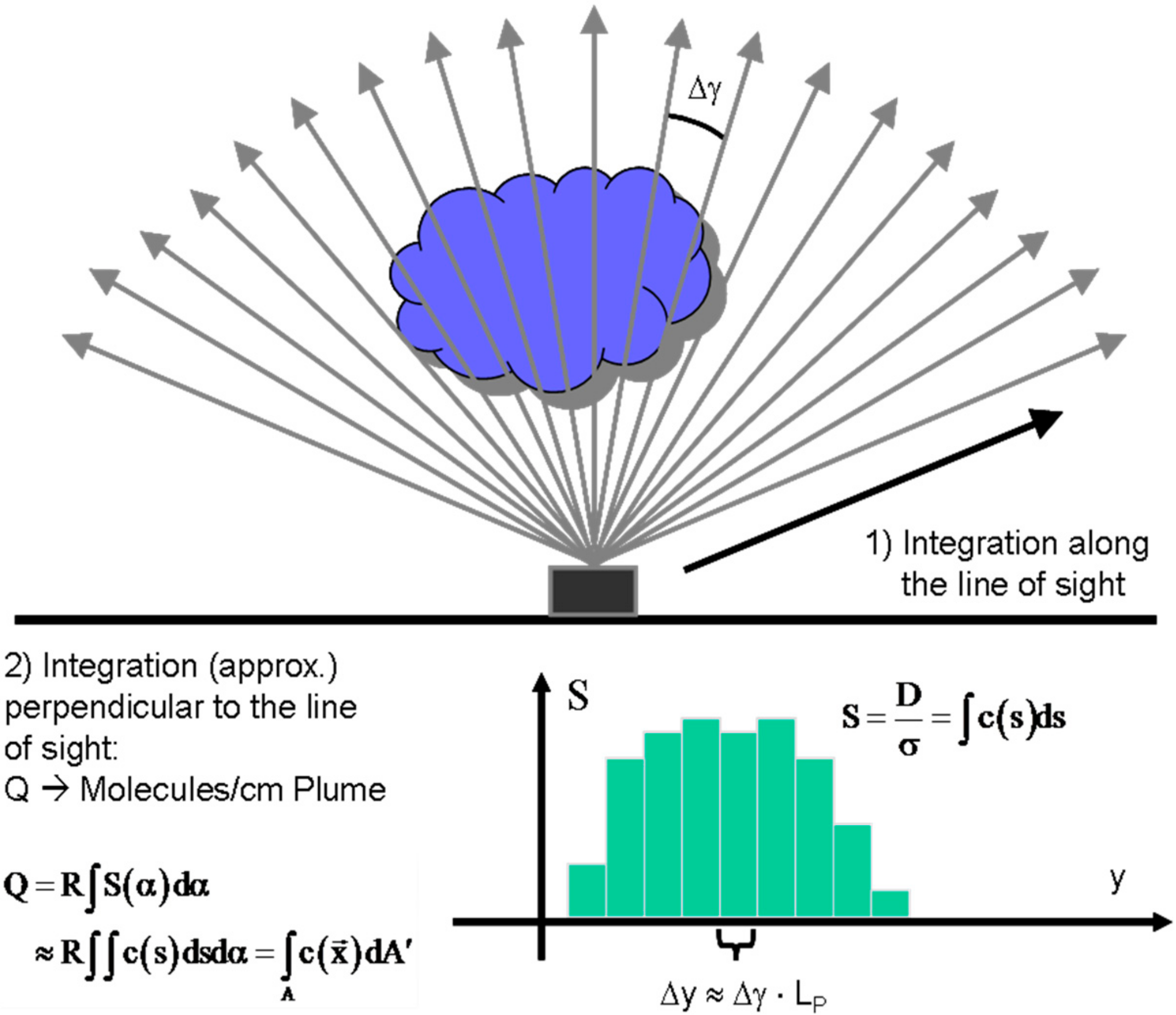
4.1. The Principle of Volcanic Gas Flux Determination

As described above, conventional one-dimensional (1-D) spectroscopic measurements typically measure the trace gas column density of the species of interest along a single line of sight. Integration of the gas concentration along this line occurs intrinsically (see Equation (6) in Section 2.1), and the measured quantity is the number of molecules along the line of sight. In order to derive an emission rate, the number of molecules Q in a cross-section of the plume perpendicular to its propagation direction is needed. Conventional 1D instruments measure this quantity by traversing under the plume or scanning the viewing direction across the plume and integrating the derived column densities (e.g., [15]).

The procedure is sketched in Figure 10 it consists of measuring a series of column densities S_i through the plume (ideally an infinite number of column densities) and integrating over the derived columns within the width w of the plume (Equation (18)).

$$\mathrm{J}={\mathrm{v}}_{\mathrm{P}}\cdot {\displaystyle \underset{\mathrm{w}}{\int }\mathrm{S}(\mathrm{y})\cdot \mathrm{d}\mathrm{y}}=\mathrm{Q}\cdot {\mathrm{v}}_{\mathrm{P}}$$

(18)

From the quantity Q the emission rate J can be readily determined by multiplication with the plume speed v_P.

While determining the position y across the plume is no problem when traversing under the plume (e.g., with a spectrometer mounted on a car) for instruments scanning the plume from a fixed point (e.g., all NOVAC stations work like this, see [10]) only the observation angle is known. In this case an estimate of the distance L_P to the plume is required and the perpendicular position y can be derived from geometrical considerations (in the simplest case as ∆y = L_P·∆γ, where Δγ is the change in scan angle).

The plume speed (i.e., wind speed v_P at the position of the plume) and the wind direction can be determined in a number of ways:

(1)

From local measurements

(2)

From large scale wind fields, which are available from regional or global data bases (e.g., ECMWF or MERRA).

(3)

From measured correlation data within the plume itself (see e.g., [18,64,94,95])

Approaches (1) and (2) suffer from various shortcomings: Local wind speed measurements at the crater rim are usually not available and wind speed measurements further away are frequently disturbed by orographic influences. Wind speeds from large scale wind fields usually are on a very coarse grid (e.g., 1° by 1°), while they are typically less affected by local orography these data may just not be representative for the site of the volcano. In contrast to that approach (3) is based on the fact that the gas (e.g., SO₂) emission strength from a volcano usually varies considerably (typically several 10%) with time on time scales of seconds to minutes as sketched in Figure 11. Thus, the column densities S₁(t) and S₂(t) are measured at two points within the plume which are located at different distances d₁ and d₂ downwind from the volcanic source (i.e., usually the crater). From the two time series the time lag ∆t_P for maximum correlation between the two time series (which typically may encompass a time period of several minutes) is calculated. From ∆t_P and the difference d₂–d₁ in downwind distance of the two measurement points the plume speed is given by:

$${\mathrm{v}}_{\mathrm{P}}=\frac{{\mathrm{d}}_2-{\mathrm{d}}_1}{\Delta {\mathrm{t}}_{\mathrm{P}}}$$

(19)

For the above reasons approach (3) is the preferred method of determining the wind speed in the plume within the NOVAC network.

Imaging techniques, however, have the advantage that they already record two spatial dimensions. Therefore, scanning is only required if the imaging technique itself is based on scanning technology (e.g., Imaging DOAS, see Section 3). Trace gas cameras (e.g., SO₂ cameras described above and in Section 3) based on band-pass filters do not require scanning. Instead, the number of SO₂ molecules Q in the plume cross-section can be derived by spatially integrating the recorded column images across the plume width w, perpendicular to the plume direction (see Figure 10). In case the plume cross-section is not taken perpendicular to its propagation direction a trigonometric correction has to be applied as described by several authors (e.g., [10,82,88]) and is discussed in detail in Section 4.2 below.

In this case the plume speed can be determined directly from the camera data through analysis of sequentially recorded images (e.g., [68,69,84,96]), providing a significant advantage over non-imaging techniques, which typically employ independent measurements of the wind speed at the appropriate plume height. Special software packages were developed e.g., by Valade et al. [97] and a direct validation of thus derived SO₂ emissions were reported by Smekens et al. [84].

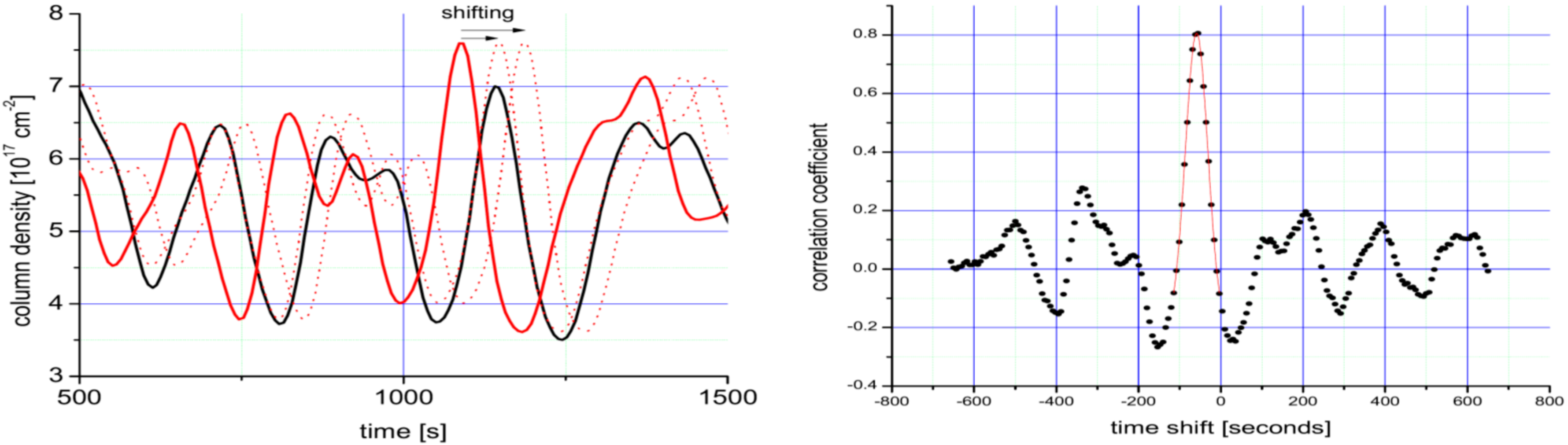
4.2. A More Detailed View—Determination of the Wind Direction

The simple approach sketched in Section 4.1—while applicable directly in certain cases—must be extended to compensate for particular conditions of the measurement:

(1)

Light dilution may affect the accuracy of the column density retrieval

(2)

Multiple scattering inside the plume can also affect the column density retrieval

(3)

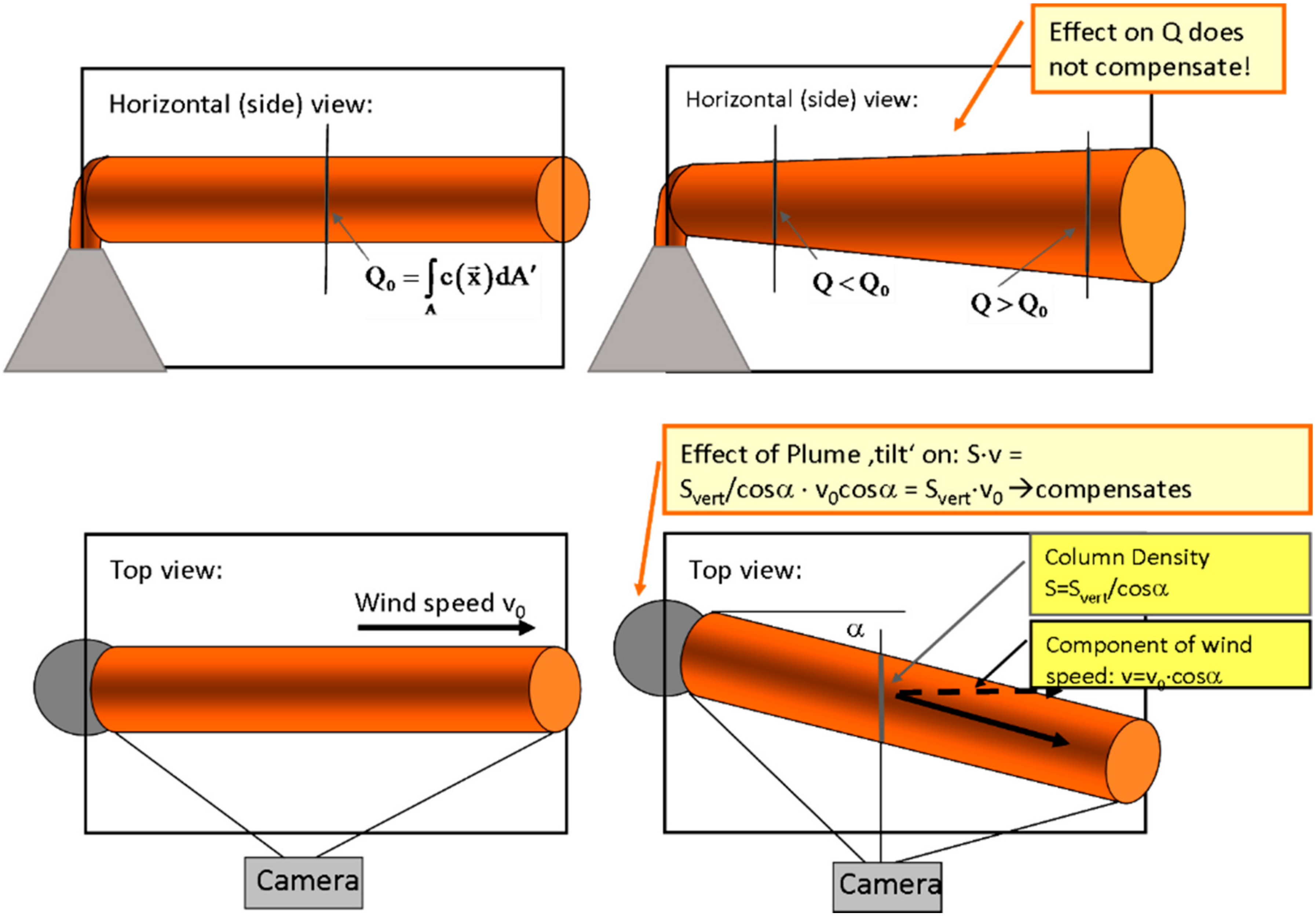
The effect of the plume propagation direction being non-perpendicular to the viewing direction must be corrected

The first two effects are discussed in several publications, e.g., [30,82,83,92,99,100] with the bottom line being that corrections are possible on the basis of a detailed analysis of the recorded trace gas (e.g., SO₂) spectra. Correction of the third effect is addressed in the following. The problem lies in the correct determination of the plume propagation direction. While this is usually not a problem when the trace gas column density is determined by a zenith looking instrument during traverses, since in these cases the position of the source (e.g., the crater) and the position of the measurement are usually well known. Consequently the angle α between the plume propagation direction (i.e., the wind direction) and the direction of the traverse is also known with high precision.

However, if measurements are made from a fixed point, either by a scanning system or a two dimensional trace gas camera (e.g., a SO₂ Camera), then the angle α between the plume propagation direction and the scanning direction or the image plane of the camera are not a priori known.

As sketched in Figure 12 there are several effects if the plume propagation direction is not perpendicular to the scanning direction or not in the image plane, respectively.

Following the discussion in Klein et al. [22], we consider data derived by a plume imaging system. For simplicity we initially also assume a cylindrical plume (i.e., a plume where the cross section does not change with distance from the origin and with time). Later we will generalize for an arbitrary plume cross section and its evolution. As can be seen in Figure 12 top view (lower left panel) in the centre of the image plane the determined flux will be independent of the “tilt” angle α between image plane and plume propagation direction. This is due to the fact that two effects cancel (as noted e.g., by Mori and Burton [96]):

(1)

The length of the light path through the plume increases as 1/cos(α).

(2)

The determined apparent wind speed is reduced by the factor cos(α) since the determined d₂–d₁ appears shorter by this factor (see bottom right panel of Figure 12) while the determined time lag ∆t_P stays the same.

However, this only holds for one point (e.g., the centre) within the field of view. Across the field of view there are two effects:

(1)

Still the light path through the plume is larger towards the edges of the image, while the determined velocity v_P stays the same. Thus the flux appears to increase somewhat towards the edges of the image compared to the centre.

(2)

A further effect of at “tilt” is due to geometry in that the closer part of the plume appears larger than the part which is further away from the camera (see top right panel of Figure 12) thus the integral (Equation (18)) will extend over a larger extent and thus be larger.

When image series (“movies”) of the plume are available these effects can be fortunately not only corrected, but rather the data can be used to determine the “tilt” angle α of the plume. This is done by (1) determining the flux in each image column of the image (where the plume is covered) and (2) making use of the usually well justified assumption that the amount of trace gas (e.g., SO₂) within the plume is conserved over a time period of a few minutes. Therefore the flux must be the same across the entire field of view (once the effect of the centre to edge enhancement (see above) is corrected for). If the thus corrected flux is not constant under the initial assumption of α = 0 then α is varied until the flux is constant across the field of view (see Figure 13).

5. Sample Applications

Technical advances in remote sensing and volcanic gas imaging have led to high temporal and spatial resolution data, which now allow the investigation of volcanic source behaviour taking place below the Earth surface by combining the surface observation of gas release with geophysical data and fluid dynamic models for melt and atmosphere including numerical models and laboratory data. Apart from the volcanological application also the volcanic plume chemistry and therefore the impact on the atmosphere can be investigated in more detail for instance by studying the heterogeneity of volcanic plumes and also by visualizing their mixing with the atmosphere. However, to our knowledge this possible application has not been realised so far. In the following section we will illustrate the new possibilities for volcanological investigations using some recent example studies.

5.1. UV Spectroscopy

Measurements of gases emitted from volcanoes, in particular the amount of SO₂, have traditionally taken place using UV-light applications, starting with COSPEC [28] in the 70s and after 2002 measurements were more widely undertaken by applying DOAS technique. However, both approaches were rarely used for two-dimensional imaging and SO₂ fluxes were determined with a time resolution of >5 min. An exception are the wide field of view UV spectrometer applications [101,102]. Highly improved time resolution and reduced error for plume velocities are possible since the onset of the SO₂ camera application [82,96]. Using an SO₂ camera leads to the determination of SO₂ emissions with time resolution of the order of a second and therefore it opens the possibility to correlate gas emission measurements directly with geophysical signals (tremor, very long period events etc.) and thus adding information to test current models of physical processes below the Earth surface.

A recent example is the work of Moussallam et al. [103], describing different degassing patterns of lava lakes in relation with their underlying conduit flow processes (See Figure 14). The authors point out that there is no similarity between gas emissions of three out of four volcanoes (Erebus, Ambrym, Kilauea, Villarica) containing lava lakes, which were all studied with a comparable time resolution. The reason proposed are differences in magma viscosity and conduit geometry, which cause the different character of emission flux behaviour. No regular periodicity of gas fluxes as well as composition could be determined in data of Villarica volcano, Chile. Those surficial gas measurements, which were combined with thermal infra-red data, point to flow instabilities inside the conduit and a turbulent mixing between the ascending gas rich and the descending gas poor magma. Part of the observed high frequency variability of the emission strength of Villarica volcano is suggested to originate from atmospheric transport processes. Instead, periodic oscillations of flux and composition were found at Erebus and Ambrym (e.g., [101,104]) indicating, combined with geophysical data, a bidirectional magma flow, whereas at Kilauea [105], oscillation of degassing amounts has been interpreted as shallow degassing patterns due to gas percolation.

However, not only has lava lake degassing been investigated so far, high time resolution SO₂ camera measurements were also done to investigate puffing and strombolian explosions at various volcanoes, showing similarly large differences in degassing characteristics of different volcanoes [19,106,107], came to the conclusion that explosions are only second order degassing processes compared with quiescent degassing. Those studies were undertaken at Stromboli and Assama volcano, respectively, showing that less than 16% of the gas amount is emitted by explosions. In contrast studies at Fuego volcano by Waite et al. [108] suggest that 95% of the total degassing amount is contributed by explosions.

Table 2. Comparison studies between SO₂ camera-derived SO₂ fluxes and geophysical parameters.

Volcano	Seismic VLP	Seismic Tremor	Acoustic	Thermal	Reference
Pacaya, Guatemala	−	−	−	−	[110]
Asama, Japan	+	−	−	−	[107]
Fuego, Guatemala	−	+ (time shifted)	−	−	[68]
Stromboli, Italy	+	−	−	−	[106]
Etna, Italy	−	+	−	−	[107]
Karymsky, Kamchatka	−	−	0	0	[111]
Fuego, Guatemala	+	−	−	−	[108]
Etna, Italy	−	+	−	−	[112]
Stromboli, Italy	−	−	−	−	[113]
Stromboli, Italy	+	−	−	−	[109]
Hawaii, USA	−	+	−	−	[105]
Etna, Italy	−	0	0	−	[114]
Stromboli, Italy	−	−	+	0	[115]
Stromboli, Italy	+	−	0	0	[116]

+: Correlation is reported; −: no correlation has been found; 0: the parameter were independently reported and used together for a volcanological interpretation no investigation of the correlation between the parameter has been presented.

is an expanded overview of the one of Burton et al. [109]. Summarizing comparison studies between SO₂ camera-derived SO₂ fluxes and some geophysical parameters.

5.2. IR Spectroscopy

Although IR techniques have complex analytical requirements and still need relatively bulky and cost intensive instruments, IR techniques are highly desirable to investigate volcanic gas compositions, because nearly all major volcanic gas compounds show characteristic absorption bands in the infra-red.

Unfortunately, the two main volcanic gases, water vapour and CO₂, although they have strong absorption features in the near IR are quite challenging to detect, mainly due to their high atmospheric background and its spatial variation. Nevertheless, the value of such information has been already demonstrated by using light path arrangements which avoid large atmospheric distances, i.e., light paths close to the source and using either artificial lamps or hot ground surfaces (e.g., lava lakes). For instance, at Erebus (e.g., [117]), Etna (e.g., [36,118,119]), Ambrym ([104]), and Stromboli (e.g., [120,121]), high frequency variations of major plume composition could be successfully determined over time frames of hours to months. Further, progress has been done during the last few years (e.g., [46,53]) and even from space volcanic CO₂ emissions of at Yasur (on Tanna Island, Vanuatu), Aoba and Ambrym volcanoes (Vanuatu) have been detected by OCO-2 [122]. Although these last examples are far from routinely usable measurements they show new technical developments for future research.

An interesting example for the advanced understanding of physical processes inside the feeding system of a volcano is the work by La Spina et al. [121]. Only with spatial and high time resolved investigations by FT-IR spectroscopy the authors could show that the previously proposed explanation of CO₂ flushing, a commonly proposed process, is unlikely in the case of Stromboli. The authors could come to this conclusion by observing the differences in the composition of the three investigated craters at Stromboli (CC, NEC, SWC) and the high H₂O/CO₂ ratios. They therefore suggested an alternative model (see Figure 15) to explain the enhanced CO₂/SO₂ ratios weeks before major explosions and the decreasing CO₂/SO₂ ratios during the hours just before this activity (without the need of CO₂ flushing) and also give an alternative explanation how a crystal pure magma may be transformed into a crystal rich one. This later fact could be explained by H₂O exsolution and crystallization driven by depressurization when magma rises to the surface. La Spina et al. [121] assume that the increase of the CO₂/SO₂ ratio is caused by more magma input into the shallow system. This should lead to a drop of permeability in the deep system which then causes the decrease of CO₂/SO₂ ratios as the mixture of deep degassing and shallow degassing is shifted to a larger percentage of shallow degassing. According to the calculation of the authors this seems far more realistic than the incredible large amounts of CO₂ needed to produce significant isobaric dehydration to reproduce the measured H₂O/CO₂ values. Further, La Spina et al. [121] utilize the observed spatial and temporal heterogeneity to produce a new model describing the geometrical structure of the shallow plumbing system of Stromboli (see Figure 15).

In contrast to the observation of [121] at Stromboli, in another study of Oppenheimer et al. [123] did not find a significant variation of the CO₂/SO₂ ratio at Yasur volcano between explosive and passive degassing activity. However, large variations (more than a magnitude) are observed in the HCl/SO₂ ratio with a ratio of about two during quiescent degassing and about 30 during explosions. These results are explained with gas accumulation below the HCl exsolution.

In addition, less abundant gases (e.g., SiF₄) where recently successfully studied using FTIR. After the first measurements of SiF₄ in a volcanic plume by Francis et al. [124], two dimensional SiF₄ distributions have been presented by [45] using thermal emission spectroscopy. Taquet et al. [125] also used thermal emission based spectroscopy to study the SiF₄/SO₂ ratio over a period of 6 month during dome growth at Popocateptl. The authors found high variability of this ratio in coincidence with seismic data. SiF₄ is a secondary gas formed due to the interaction of HF with rocks or ash. Nevertheless, there is a high potential to study certain types of activity (e.g., dome growth) and eventually using this approach for monitoring in the future. In the article by Taquet et al. [125] the variation of the SiF₄, SO₂ and the ratio SiF₄/SO₂ helped to decipher the different processes related to the dome permeability.

6. Summary and Outlook

There is a clear development from occasional volcanic gas concentration measurements (typically by “wet” chemical techniques or gas chromatography) to continuous observations as pioneered by the COSPEC technique (e.g., [28]) and brought to a large scale by the NOVAC network (e.g., [10]) and other local networks (e.g., [109,126]). In addition gas concentration (or column density) measurements have been extended to flux measurements (see e.g., NOVAC). Another dimension is marked by the extension of SO₂ measurements to continuous multi-species observations. In this context also extremely affordable spectrometers based on mass produced smart phone imagers [127] can play a role.

From here a next quantitative jump (or paradigm shift, see [16]) is marked by gas imaging techniques like the SO₂ camera (see e.g., [109]), which allow—compared to scanning approaches—a much more detailed analysis of volcanic emissions and plume behaviour. Besides more precise flux measurements for instance short term periodicity in emission flux [16] or the angle between plume direction and image plane can be derived. Moreover, the spatial inhomogeneity of volcanic sources can be investigated.

High Frequency imaging of volcanic plumes was first realized with UV cameras and instruments based on this technique can be produced rather cost effectively and—as was recently shown by Wilkes et al. [128] have the potential to become very cheap instruments which may be ubiquitous in volcanic research. However, the approach has two drawbacks.

(1)

The relatively crude spectroscopic approach, basically just ratioing the intensities in two wavelength intervals leads to interferences by aerosol, (stratospheric) ozone, and possibly other species. Moreover, radiation transport issues may also influence the accuracy of the technique (see e.g., [71,82,129]).

(2)

UV cameras rely on sunlight and can thus only operate during daylight hours.

There are techniques under development (or being adapted for the purpose of volcanic observations) which promise to overcome these weaknesses. These include gas correlation spectroscopy (see Section 3.4), titled filter imaging, and Fabry Pérot imaging (see [79,80]), which both make better use of the spectral finger print of the target gas than the classic UV camera, thus reducing interferences and potentially improving the accuracy of the measurement (see also [5]).

Infra-red thermal emission spectroscopy is independent of daylight and may be the technology of the future in either scanning or imaging applications. At present cost and logistic requirements (cooling of the IR detector, use of interferometers with moving parts) are still high. Here technological development aimed at lowering complexity and cost of the instruments would be very welcome.

At present, imaging Michelson interferometers exist and are used for certain purposes, but the instruments are still extremely expensive. Alternatively, the UV-camera approach can be extended to the thermal IR region (see e.g., [56]), while this approach suffers from similar problems as the UV camera (see above) the rapidly falling prices of thermal IR cameras may make this approach feasible for volcanological applications.

With all spectroscopic techniques radiation transport issues are important and may be limiting the achievable accuracy (see Section 2). Here, better radiation transport models and new approaches like using polarisation of the radiation and ratioing techniques based on the absorption due to “known” absorbers like O₂ or O₄ (oxygen dimers, see e.g., [130,131]) will be helpful.

Overall, it becomes clear that spectroscopic plume analysis is just at the beginning of its development and it constitutes a new and rapidly evolving technique to analyze magmatic degassing, which is (coupled with viscosity and crystallisation) the main driver of volcanic processes.

References

1. Robock, A. Volcanic Eruptions and Climate. Rev. Geophys. 2000, 38, 191–219. [Google Scholar] [CrossRef]
2. Von Glasow, R.; Bobrowski, N.; Kern, C. The effects of volcanic eruptions on atmospheric chemistry. Chem. Geol. 2009, 263, 131–142. [Google Scholar] [CrossRef]
3. Kutterolf, S.; Hansteen, T.H.; Appel, K.; Freundt, A.; Krüger, K.; Pérez, W.; Wehrmann, H. Combined bromine and chlorine release from large explosive volcanic eruptions: A threat to stratospheric ozone? Geology 2013, 41, 707–710. [Google Scholar] [CrossRef]
4. Platt, U.; Bobrowski, N. Quantification of volcanic reactive halogen emissions. In Volcanism and Global Change; Schmidt, A., Fristad, K., Elkins-Tanton, L., Eds.; Cambridge University Press: Cambridge, UK, 2015; ISBN 9781107058378. [Google Scholar]
5. Platt, U.; Lübcke, P.; Kuhn, J.; Bobrowski, N.; Prata, F.; Burton, M.R.; Kern, C. Quantitative Imaging of Volcanic Plumes—Results, Future Needs, and Future Trends. J. Volcanol. Geotherm. Res. 2015, 300, 7–21. [Google Scholar] [CrossRef]
6. Noguchi, K.; Kamiya, H. Prediction of volcanic eruption by measuring the chemical composition and amounts of gases. Bull. Volcanol. 1963, 26, 367–378. [Google Scholar] [CrossRef]
7. Malinconico, L.L., Jr. On the Variation of SO2 emission from volcanoes. J. Volcanol. Geotherm. Res. 1987, 33, 231–237. [Google Scholar] [CrossRef]
8. Sutton, A.J.; Elias, T.; Gerlach, T.M.; Stokes, J.B. Implications for eruptive proecesses as indicated by sulfur dioxide emissions from Kilauea Volcano, Hawai’i, 1979–1997. J. Volcanol. Geotherm. Res. 2001, 108, 283–302. [Google Scholar] [CrossRef]
9. Burton, M.R.; Allard, P.; Mure, F.; Oppenheimer, C. FTIR remote sensing of fractional magma degassing at Mt. Etna, Sicily. Geol. Soc. 2003, 213, 281–293. [Google Scholar] [CrossRef]
10. Galle, B.; Johansson, M.; Rivera, C.; Zhang, Y.; Kihlman, M.; Kern, C.; Lehmann, T.; Platt, U.; Arellano, S.; Hidalgo, S. Network for Observation of Volcanic and Atmospheric Change (NOVAC)—A global network for volcanic gas monitoring: Network layout and instrument description. J. Geophys. Res. 2010, 115, D05304. [Google Scholar] [CrossRef]
11. Lübcke, P.; Bobrowski, N.; Arellano, S.; Galle, B.; Garzon, G.; Vogel, L.; Platt, U. BrO/SO2 ratios from the NOVAC Network. Solid Earth 2014, 5, 409–424. [Google Scholar] [CrossRef]
12. Dinger, F.; Bobrowski, N.; Warnach, S.; Bredemeyer, S.; Hidalgo, S.; Arellano, S.; Galle, B.; Platt, U.; Wagner, T. Periodicity in the BrO/SO2 molar ratios in volcanic gas plumes and its correlation with the Earth tides, Part 1: Observation during the Cotopaxi eruption 2015. Solid Earth Discuss. 2017. [Google Scholar] [CrossRef]
13. Weibring, P.; Andersson, M.; Edner, H.; Svanberg, S. Remote Monitoring of Industrial Emissions by Combination of Lidar and Plume Velocity Measurements. Appl. Phys. B 1998, 66, 383–388. [Google Scholar] [CrossRef]
14. Weibring, P.; Swartling, J.; Edner, H.; Svanberg, S.; Caltabiano, T.; Condarelli, D.; Cecchi, G.; Pantani, L. Optical Monitoring of Volcanic Sulphur Dioxide Emissions—Comparison between four Different Remote Sensing Techniques. Opt. Lasers Eng. 2002, 37, 267–284. [Google Scholar] [CrossRef]
15. Galle, B.; Oppenheimer, C.; Geyer, A.; McGonigle, A.J.; Edmonds, M.; Horrocks, L. A miniaturised ultraviolet spectrometer for remote sensing of SO2 fluxes: A new tool for volcano surveillance. J. Volcanol. Geotherm. Res. 2003, 119, 241–254. [Google Scholar] [CrossRef]
16. McGonigle, A.J.S.; Pering, T.D.; Wilkes, T.C.; Tamburello, G.; D’Aleo, R.; Bitetto, M.; Aiuppa, A.; Willmott, J.R. Ultraviolet Imaging of Volcanic Plumes: A New Paradigm in Volcanology. Geosciences 2017, 7, 68. [Google Scholar] [CrossRef]
17. McGonigle, A.J.S.; Hilton, D.R.; Fischer, T.P.; Oppenheimer, C. Plume velocity determination for volcanic SO2 flux measurements. Geophys. Res. Lett. 2005, 32, L11302. [Google Scholar] [CrossRef]
18. McGonigle, A.J.S.; Inguaggiato, S.; Aiuppa, A.; Hayes, A.R.; Oppenheimer, C. Accurate measurement of volcanic SO2 flux: Determination of plume transport speed and integrated SO2 concentration with a single device. Geochem. Geophys. Geosyst. 2005, 6, Q02003. [Google Scholar] [CrossRef]
19. Mori, T.; Burton, M. Quantification of the gas mass emitted during single explosions on Stromboli with the SO2 imaging camera. J. Volcanol. Geotherm. Res. 2009, 188, 395–400. [Google Scholar] [CrossRef]
20. Kern, C.; Sutton, J.; Elias, T.; Lee, L.; Kamibayashi, K.; Antolik, L.; Werner, C. An automated SO2 camera system for continuous, real-time monitoring of gas emissions from Klauea Volcano’s summit Overlook Crater. J. Volcanol. Geotherm. Res. 2015, 300, 81–94. [Google Scholar] [CrossRef]
21. Peters, N.; Hoffmann, A.; Barnie, T.; Herzog, M.; Oppenheimer, C. Use of motion estimation algorithms for improved flux measurements using SO2 cameras. J. Volcanol. Geotherm. Res. 2015, 300, 58–69. [Google Scholar] [CrossRef]
22. Klein, A.; Lübcke, P.; Bobrowski, N.; Kuhn, J.; Platt, U. Plume Propagation Direction Determination with SO2 Cameras. Atmos. Meas. Tech. 2017, 10, 979–987. [Google Scholar] [CrossRef]
23. General, S.; Pöhler, D.; Sihler, H.; Bobrowski, N.; Frieß, U.; Zielcke, J.; Horbanski, M.; Shepson, P.; Stirm, B.; Simpson, W.; et al. The Heidelberg Airborne Imaging DOAS Instrument (HAIDI) A Novel Imaging DOAS Device for 2-D and 3-D Imaging of Trace Gases. J. Atmos. Meas. Tech. 2014, 7, 3459–3485. [Google Scholar] [CrossRef]
24. Krueger, A.J. Sighting of El Chichon sulfur dioxide clouds with the Nimbus 7 Total Ozone Mapping Spectrometer. Science 1983, 220, 1377–1378. [Google Scholar] [CrossRef] [PubMed]
25. Hörmann, C.; Sihler, H.; Bobrowski, N.; Beirle, S.; Penning de Vries, M.; Platt, U.; Wagner, T. Systematic investigation of bromine monoxide in volcanic plumes from space by using the GOME-2 instrument. Atmos. Chem. Phys. 2013, 13, 4749–4781. [Google Scholar] [CrossRef]
26. Carn, S.A.; Clarisse, L.; Prata, A.J. Multi-decadal satellite measurements of global volcanic degassing. J. Volcanol. Geotherm. Res. 2016, 311, 99–134. [Google Scholar] [CrossRef]
27. Platt, U.; Stutz, J. Differential Optical Absorption Spectroscopy, Principles and Applications; Springer: Heidelberg, Germany, 2008; p. 597. ISBN 978-3-540-21193-8. [Google Scholar]
28. Moffat, A.J.; Millán, M.M. The application of optical correlation techniques to the remote sensing of SO2 plumes using sky light. Atmos. Environ. 1971, 5, 677–690. [Google Scholar] [CrossRef]
29. Lübcke, P.; Lampel, J.; Arellano, S.; Bobrowski, N.; Dinger, F.; Galle, B.; Garzón, G.; Hidalgo, S.; Ortiz, Z.C.; Vogel, L. Retrieval of absolute SO2 column amounts from scattered-light spectra—Implications for the evaluation of data from automated DOAS Networks. Atmos. Meas. Tech. 2016, 9, 5677–5698. [Google Scholar] [CrossRef]
30. Kern, C.; Sihler, H.; Vogel, L.; Rivera, C.; Herrera, M.; Platt, U. Halogen oxide measurements at Masaya volcano, Nicaragua using Active Long Path Differential Optical Absorption Spectroscopy. Bull. Volcanol. 2009, 71, 659–670. [Google Scholar] [CrossRef]
31. Vita, F.; Kern, C.; Inguaggiato, S. Development of a portable active long-path differential optical absorption spectroscopy system for volcanic gas measurements. J. Sens. Sens. Syst. 2014, 3, 355–367. [Google Scholar] [CrossRef]
32. Horton, K.A.; Williams-Jones, G.; Garbeil, H.; Elias, T.; Sutton, A.J.; Mouginis-Mark, P.; Porter, J.N.; Clegg, S. Real-time measurement of volcanic SO2 emissions: Validation of a new UV correlation spectrometer (FLYSPEC). Bull. Volcanol. 2005, 68, 323–327. [Google Scholar] [CrossRef]
33. Mori, T.; Notsu, K. Remote CO, COS, CO2, SO2, HCl detection and temperature estimation of volcanic gas. Geophys. Res. Lett. 1997, 24, 2047–2050. [Google Scholar] [CrossRef]
34. Oppenheimer, C.; Francis, P.; Burton, M.; Maciejewski, A.; Boardman, L. Remote measurement of volcanic gases by Fourier transform infrared spectroscopy. Appl. Phys. B 1998, 67, 505–515. [Google Scholar] [CrossRef]
35. Burton, M.R.; Oppenheimer, C.; Horrock, L.A.; Francis, P.W. Remote sensing of CO2 and H2O emission rates from Masaya volcano, Nicaragua. Geology 2000, 28, 915–918. [Google Scholar] [CrossRef]
36. Allard, P.; Burton, M.; Muré, F. Spectroscopic evidence for a lava fountain driven by previously accumulated magmatic gas. Nature 2005, 433, 407–410. [Google Scholar] [CrossRef] [PubMed]
37. Carapezza, M.L.; Barberi, F.; Ranaldi, M.; Ricci, T.; Tarchini, L.; Barrancos, J.; Fischer, L.C.; Perez, N.; Weber, K.; Gattuso, A.; et al. Diffuse CO2 soil degassing and CO2 and H2S concentrations in air and related hazards at Vulcano Island (Aeolian arc, Italy). J. Volcanol. Geotherm. Res. 2011, 207, 130–144. [Google Scholar] [CrossRef]
38. Pedone, M.; Aiuppa, A.; Giudice, G.; Grassa, F.; Cardellini, C.; Chiodini, G.; Valenza, M. Volcanic CO2 flux measurement at Campi Flegrei by tunable diode laser absorption spectroscopy. Bull. Volcanol. 2015, 76, 812. [Google Scholar] [CrossRef]
39. Chiarugi, A.; Viciani, S.; D’Amato, F.; Burton, M. Diode laser-based gas analyser for the simultaneous measurement of CO2 and HF in volcanic plumes. Atmos. Meas. Tech. 2018, 11, 329–339. [Google Scholar] [CrossRef]
40. Weidmann, D.; Wysocki, G.; Oppenheimer, C.; Tittel, F.K. Development of a compact quantum cascade laser spectrometer for field measurements of CO2 isotopes. Appl. Phys. B Lasers Opt. 2005, 80, 255–260. [Google Scholar] [CrossRef]
41. Richter, D.; Erdelyi, M.; Curl, R.F.; Tittel, F.K.; Oppenheimer, C.; Duffell, H.J.; Burton, M. Field measurements of volcanic gases using tunable diode laser based mid-infrared and Fourier transform infrared spectrometers. Opt. Lasers Eng. 2002, 37, 171–186. [Google Scholar] [CrossRef]
42. Waxman, E.M.; Cossel, K.C.; Truong, G.-W.; Giorgetta, F.R.; Swann, W.C.; Coburn, S.; Wright, R.J.; Rieker, G.B.; Coddington, I.; Newbury, N.R. Intercomparison of open-path trace gas measurements with two dual-frequency-comb spectrometers. Atmos. Meas. Tech. 2017, 10, 3295–3311. [Google Scholar] [CrossRef] [PubMed]
43. Francis, P.; Burton, M.R.; Oppenheimer, C. Remote measurements of volcanic gas compositions by solar occultation spectroscopy. Nature 1998, 396, 567–570. [Google Scholar] [CrossRef]
44. Burton, M.R.; Oppenheimer, C.; Horrocks, L.A.; Francis, P.W. Diurnal changes in volcanic plume chemistry observed by lunar and solar occultation spectroscopy. Geophys. Res. Lett. 2001, 28, 843–846. [Google Scholar] [CrossRef]
45. Duffell, H.; Oppenheimer, C.; Burton, M. Volcanic gas emission rates measured by solar occultation spectroscopy. Geophys. Res. Lett. 2001, 28, 3131–3134. [Google Scholar] [CrossRef]
46. Butz, A.; Dinger, A.S.; Bobrowski, N.; Kostinek, J.; Fieber, L.; Fischerkeller, C.; Giuffrida, G.B.; Hase, F.; Klappenbach, F.; Kuhn, J.; et al. Remote sensing of volcanic CO2, HF, HCl, SO2, and BrO in the downwind plume of Mt. Etna. Atmos. Meas. Tech. 2017, 10, 1–14. [Google Scholar] [CrossRef]
47. Naughton, J.J.; Derby, J.V.; Glover, R.B. Infrared measurements on volcanic gas and fume: Kilauea eruption, 1968. J. Geophys. Res. 1969, 74, 3273–3277. [Google Scholar] [CrossRef]
48. Mori, T.; Notsu, K.; Tohjima, Y.; Wakita, H. Remote detection of HCl and SO2 in volcanic gas from Unzen volcano, Japan. Geophys. Res. Lett. 1993, 20, 1355–1358. [Google Scholar] [CrossRef]
49. Notsu, K.; Mori, T.; Igarishi, G.; Tohjima, Y.; Wakita, H. Infrared spectral radiometer: A new tool for remote measurement of SO2 of volcanic gas. Geochem. J. 1993, 27, 361–366. [Google Scholar] [CrossRef]
50. Mori, T.K.; Notsu, Y.; Tohjima, H.; Wakita, P.M.; Nuccio, M.; Italiano, F. Remote detection of fumarolic gas chemistry at Vulcano, Italy, using an FT-IR spectral radiometer. Earth Planet. Sci. Lett. 1995, 134, 219–224. [Google Scholar] [CrossRef]
51. Gerlach, T.M.; McGee, K.A.; Elias, T.; Sutton, A.J.; Doukas, M.P. Carbon dioxide emission rate of Kilauea Volcano: Implications for primary magma and the summit reservoir. J. Geophys. Res. 2002, 107, 2189. [Google Scholar] [CrossRef]
52. Aiuppa, A.; Fiorani, L.; Santoro, S.; Parracino, S.; Nuvoli, M.; Chiodini, G.; Minopoli, C.; Tamburello, G. New groundbased lidar enables volcanic CO2 flux measurements. Sci. Rep. 2015, 5, 13614. [Google Scholar] [CrossRef] [PubMed] [Green Version]
53. Queisser, M.; Burton, M.; Allan, G.; Chiarugi, A. Portable laser spectrometer for airborne and ground-based remote sensing of geological CO2 emissions. Opt. Lett. 2017, 42, 2782–2785. [Google Scholar] [CrossRef] [PubMed]
54. Goff, F.; Love, S.P.; Warren, R.G.; Counce, D.; Obenholzner, J.; Siebe, C.; Schmidt, S.C. Passive infrared remote sensing evidence for large, intermittent CO2 emissions at Popocatépetl volcano, Mexico. Chem. Geol. 2001, 177, 133–156. [Google Scholar] [CrossRef]
55. Stremme, W.; Krueger, A.; Harig, R.; Grutter, M. Volcanic SO2 and SiF4 visualization using 2-D thermal emission spectroscopy-Part 1: Slant-columns and their ratios. Atmos. Meas. Tech. 2012, 5, 275–288. [Google Scholar] [CrossRef]
56. Prata, A.; Bernardo, C. Retrieval of sulphur dioxide froma ground-based thermal infrared imaging camera. Atmos. Meas. Tech. 2014, 7, 2807–2828. [Google Scholar] [CrossRef]
57. Gabrieli, A.; Wright, R.; Lucey, P.G.; Porter, J.N.; Garbeil, H.; Pilger, E.; Wood, M. Characterization and initial field test of an 8–14 μm thermal infrared hyperspectral imager for measuring SO2 in volcanic plumes. Bull. Volcanol. 2016, 78, 73. [Google Scholar] [CrossRef]
58. Love, S.P.; Goff, F.; Counce, D.; Siebe, C.; Delgado, H. Passive infrared spectroscopy of the eruption plume at Popocatepetl volcano, Mexico. Nature 1998, 396, 563–567. [Google Scholar] [CrossRef]
59. Krueger, A.; Stremme, W.; Harig, R.; Grutter, M. Volcanic SO2 and SiF4 visualization using 2-D thermal emission spectroscopy—Part 2: Wind propagation and emission rates. Atmos. Meas. Tech. 2013, 6, 47–61. [Google Scholar] [CrossRef]
60. Friedl-Vallon, F.; Gulde, T.; Hase, F.; Kleinert, A.; Kulessa, T.; Maucher, G.; Neubert, T.; Olschewski, F.; Piesch, C.; Preusse, P.; et al. Instrument concept of the imaging Fourier transform spectrometer GLORIA. Atmos. Meas. Tech. 2014, 7, 3565–3577. [Google Scholar] [CrossRef]
61. Hinkley, E.D. (Ed.) Laser Monitoring of the Atmosphere; Topics in Applied Physics; Springer: Berlin/Heidelberg, Germany, 1976; Volume 14. [Google Scholar]
62. Svanberg, S. Atomic and Molecular Spectroscopy, 2nd ed.; Springer Series on Atoms and Plasmas; Springer: Berlin/Heidelberg, Germany, 1992. [Google Scholar]
63. Edner, H.; Ragnarson, P.; Svanberg, S.; Wallinder, E.; Ferrara, R.; Cioni, R.; Raco, B.; Taddeucci, G. Total Fluxes of Sulphur Dioxide from the Italian Volcanoes Etna, Stromboli and Vulcano Measured by Differential Absorption Lidar and Passive Differential Optical Absorption Spectroscopy. J. Geophys. Res. 1994, 99, 18827–18838. [Google Scholar] [CrossRef]
64. Weibring, P.; Edner, H.; Svanberg, S.; Cecchi, G.; Pantani, L.; Ferrara, R.; Caltabiano, T. Monitoring of Volcanic Sulphur Dioxide Emissions using Differential Absorption Lidar (DIAL), Differential Optical Absorption Spectroscopy (DOAS) and Correlation Spectroscopy (COSPEC). Appl. Phys. B 1998, 67, 419–426. [Google Scholar] [CrossRef]
65. Weckwerth, T.M.; Weber, K.J.; Turner, D.D.; Spuler, S.M. Validation of a Water Vapor Micropulse Differential Absorption Lidar (DIAL). J. Atmos. Ocean Technol. 2016, 33, 2353–2372. [Google Scholar] [CrossRef]
66. Barnes, J.E.; Bronner, S.; Beck, R.; Parikh, N.C. Boundary layer scattering measurements with a charge-coupled device camera lidar. Appl. Opt. 2003, 42, 2647–2652. [Google Scholar] [CrossRef] [PubMed]
67. Flock, S. LED-Lidar—Theoretische und Experimentelle Machbarkeitsstudie zur Realisierung Eines Bistatischen, LED-Basierten Lidarsystems. Master’s Thesis, University of Heidelberg, Heidelberg, Germany, 2012. (In German). [Google Scholar]
68. Nadeau, P.A.; Palma, J.L.; Waite, G.P. Linking Volcanic Tremor, Degassing, and Eruption Dynamics via SO2 Imaging. Geophys. Res. Lett. 2011, 38, 1. [Google Scholar] [CrossRef]
69. Kern, C.; Lübcke, P.; Bobrowski, N.; Campion, R.; Mori, T.; Smekens, J.-F.; Stebel, K.; Tamburello, G.; Burton, M.; Platt, U.; et al. Intercomparison of SO2 camera systems for imaging volcanic gas plumes. J. Volcanol. Geotherm. Res. 2015, 300, 22–36. [Google Scholar] [CrossRef]
70. Gliß, J.; Stebel, K.; Kylling, A.; Sudbø, A. Optical flow gas velocity analysis in plumes using UV cameras—Implications for SO2-emission-rate retrievals investigated at Mt. Etna, Italy, and Guallatiri, Chile. Atmos. Meas. Tech. Discuss. 2017. [Google Scholar] [CrossRef]
71. Lübcke, P.; Bobrowski, N.; Illing, S.; Kern, C.; Vogel, L.; Platt, U. On the absolute calibration of SO2 Cameras. Atmos. Meas. Tech. 2013, 6, 677–696. [Google Scholar] [CrossRef]
72. Rusch, P.; Harig, R. 3-D Reconstruction of Gas Clouds by Scanning Imaging IR Spectroscopy and Tomography. IEEE Sens. J. 2010, 10, 599–603. [Google Scholar] [CrossRef]
73. Lohberger, F.; Hönninger, G.; Platt, U. Ground Based Imaging Differential Optical Absorption Spectroscopy of Atmospheric Gases. Appl. Opt. 2004, 43, 4711–4717. [Google Scholar] [CrossRef] [PubMed]
74. Bobrowski, N.; Hönninger, G.; Lohberger, F.; Platt, U. IDOAS: A new monitoring technique to study the 2D distribution of volcanic gas emissions. J. Volcanol. Geotherm. Res. 2006, 150, 329–338. [Google Scholar] [CrossRef]
75. Louban, I.; Bobrowski, N.; Rouwet, D.; Inguaggiato, S.; Platt, U. Imaging DOAS for Volcanological Applications. Bull. Volcanol. 2009, 71, 753–765. [Google Scholar] [CrossRef]
76. Lee, H.-L.; Kim, J.-H.; Ryu, J.; Kwon, S.; Noh, Y.; Gu, M. 2-dimensional Mapping of Sulfur Dioxide and Bromine Oxide at the Sakurajima Volcano with a Ground Based Scanning Imaging Spectrograph System. J. Opt. Soc. Korea 2010, 14, 204–208. [Google Scholar] [CrossRef]
77. Wright, R.; Lucey, P.; Crites, S.; Horton, K.; Wood, M.; Garbeil, H. BBM/EM design of the thermal hyperspectral imager: An instrument for remote sensing of Earth’s surface, atmosphere and ocean, from a microsatellite platform. Acta Astronaut. 2013, 87, 182–192. [Google Scholar] [CrossRef]
78. Gabrieli, A.; Porter, J.N.; Wright, R.; Lucey, P.G. Validating the accuracy of SO2 gas retrievals in the thermal infrared (8–14 μm). Bull. Volcanol. 2017, 79, 80. [Google Scholar] [CrossRef]
79. Kuhn, J.; Bobrowski, N.; Lübcke, P.; Vogel, L.; Platt, U. A Fabry-Pérot Interferometer Based Camera for the two-dimensional Mapping of SO2-Distributions. J. Atmos. Meas. Tech. 2014, 7, 3705–3715. [Google Scholar] [CrossRef]
80. Kuhn, J.; Platt, U.; Bobrowski, N.; Lübcke, P.; Wagner, T. Fabry-Perot interferometer based imaging of atmospheric trace gases. In Proceedings of the 10th EARSeL SIG Imaging Spectroscopy Workshop, Zurich, Switzerland, 19–21 April 2017. [Google Scholar]
81. Eisenhauer, F.; Raab, W. Visible/infrared imaging spectroscopy and energy-resolving detectors. Annu. Rev. Astron. Astrophys. 2015, 53, 155–197. [Google Scholar] [CrossRef]
82. Bluth, G.J.S.; Shannon, J.M.; Watson, I.M.; Prata, A.J.; Realmuto, V.J. Development of an ultra-violet digital camera for volcanic SO2 imaging. J. Volcanol. Geotherm. Res. 2007, 161, 47–56. [Google Scholar] [CrossRef]
83. Kern, C.; Deutschmann, T.; Werner, C.; Sutton, A.J.; Elias, T.; Kelly, P.J. Improving the accuracy of SO2 column densities and emission rates obtained from upward-looking UV-spectroscopic measurements of volcanic plumes by taking realistic radiative transfer into account. J. Geophys. Res. 2012, 117, D20302. [Google Scholar] [CrossRef]
84. Smekens, J.-F.; Burton, M.R.; Clarke, A.B. Validation of the SO2 Camera for High Temporal and Spatial Resolution Monitoring of SO2 Emissions. J. Volcanol. Geotherm. Res. 2015, 300, 37–47. [Google Scholar] [CrossRef]
85. Prata, A.; Bernardo, C. Retrieval of volcanic ash particle size, mass and optical depth from a ground-based thermal infrared camera. J. Volcanol. Geotherm. Res. 2009, 186, 91–107. [Google Scholar] [CrossRef]
86. Lopez, T.; Thomas, H.E.; Prata, A.J.; Amigo, A.; Fee, D.; Moriano, D. Volcanic plume characteristics determined using an infrared imaging camera. J. Volcanol. Geotherm. Res. 2015, 300, 148–166. [Google Scholar] [CrossRef]
87. Sandsten, J.; Edner, H.; Svanberg, S. Gas imaging by infrared gas-correlation spectrometry. Opt. Lett. 1996, 21, 1945–1947. [Google Scholar] [CrossRef] [PubMed]
88. Sandsten, J.; Edner, H.; Svanberg, S. Gas visualization of industrial hydrocarbon emissions. Opt. Express 2004, 12, 1443–1451. [Google Scholar] [CrossRef] [PubMed]
89. Prata, A. Infrared radiative transfer calculations for volcanic ash clouds. Geophys. Res. Lett. 1989, 16, 1293–1296. [Google Scholar] [CrossRef]
90. Levelt, P.F.; Hilsenrath, E.; Leppelmeier, G.W.; van Den Oord, G.H.J.; Bhartia, P.K.; Tamminen, J.; De Haan, J.F.; Veefkind, P. Science Objectives of the Ozone Monitoring Instrument. Geosci. Remote Sens. 2006, 44, 1199–1208. [Google Scholar] [CrossRef]
91. General, S.; Bobrowski, N.; Pöhler, D.; Weber, K.; Fischer, C.; Platt, U. Airborne I-DOAS measurements at Mt. Etna BrO and OClO evolution in the plume. J. Volcanol. Geotherm. Res. 2015, 300, 175–186. [Google Scholar] [CrossRef]
92. Kern, C.; Deutschmann, T.; Vogel, L.; Wöhrbach, M.; Wagner, T.; Platt, U. Radiative transfer corrections for accurate spectroscopic measurements of volcanic gas emissions. Bull. Volcanol. 2010, 72, 233–247. [Google Scholar] [CrossRef]
93. Ward, T.V.; Zwick, H.H. Gas cell correlation spectrometer: GASPEC. Appl. Opt. 1975, 14, 2896–2904. [Google Scholar] [CrossRef] [PubMed]
94. Bobrowski, N. Volcanic Gas Studies by Multi Axis Differential Optical Absorption Spectroscopy. Diploma Thesis, University of Heidelberg, Heidelberg, Germany, 2002. [Google Scholar]
95. Johansson, M.; Galle, B.; Zhang, Y.; Rivera, C.; Chen, D.; Wyser, K. The dual-beam mini-DOAS technique—Measurements of volcanic gas emission, plume height and plume speed with a single instrument. Bull. Volcanol. 2009, 71, 747–751. [Google Scholar] [CrossRef]
96. Mori, T.; Burton, M. The SO2 camera: A simple, fast and cheap method for ground-based imaging of SO2 in volcanic plumes. Geophys. Res. Lett. 2006, 33. [Google Scholar] [CrossRef]
97. Valade, S.A.; Harris, A.J.L.; Cerminara, M. Plume Ascent Tracker: Interactive Matlab Software for Analysis of Ascending Plume. Comput. Geosci. C 2014, 66, 132–144. [Google Scholar] [CrossRef]
98. Fickel, M. Measurement of Trace Gas Fluxes from Point Sources with Multi-Axis Differential Optical Absorption Spectroscopy. Diploma Thesis, University of Heidelberg, Heidelberg, Germany, 2008. [Google Scholar]
99. Millán, M.M. Remote sensing of Air Pollutants. A Study of some Atmospheric Scattering Effects. Atmos. Environ. 1980, 14, 1241–1253. [Google Scholar] [CrossRef]
100. Kern, C. Spectroscopic Measurements of Volcanic Gas Emissions in the Ultra-Violet Wavelength Region. Ph.D. Thesis, Institute of Environmental Physics, The Faculty of Physics and Astronomy, University of Heidelberg, Heidelberg, Germany, 2009. [Google Scholar] [CrossRef]
101. Boichu, M.; Oppenheimer, C.; Tsanev, V.; Kyle, P.R. High temporal resolution SO2 flux measurements at Erebus volcano, Antarctica. J. Volcanol. Geotherm. Res. 2010, 190, 325–336. [Google Scholar] [CrossRef]
102. McGonigle, A.J.S.; Aiuppa, A.; Ripepe, M.; Kantzas, E.P.; Tamburello, G. Spectroscopic capture of 1 Hz volcanic SO2 fluxes and integration with volcano geophysical data. Geophys. Res. Lett. 2009, 36, L21309. [Google Scholar] [CrossRef]
103. Moussallam, Y.; Philipson, B.; Curtis, A.; Barnie, T.; Moussallam, M.; Peters, N.; Schipper, C.I.; Aiuppa, A.; Giudice, G.; Amigo, A.; et al. Sustaining persistent lava lakes: Observations from high-resolution gas measurements at Villarrica volcano, Chile. Earth Planet. Sci. Lett. 2016, 454, 237–247. [Google Scholar] [CrossRef]
104. Allard, P.; Burton, M.; Sawyer, G.; Bani, P. Degassing dynamics of basaltic lava lake at a top-ranking volatile emitter: Ambrym volcano, Vanuatu arc. Earth Planet. Sci. Lett. 2016, 448, 69–80. [Google Scholar] [CrossRef]
105. Nadeau, P.A.; Werner, C.A.; Waite, G.P.; Carn, S.A.; Brewer, I.D.; Elias, T.; Sutton, A.J.; Kern, C.; Patrick, M.R. Using SO2 camera imagery and seismicity to examine degassing and gas accumulation at Kīlauea Volcano, May 2010. J. Volcanol. Geotherm. Res. 2015, 300, 70–80. [Google Scholar] [CrossRef]
106. Tamburello, G.; Aiuppa, A.; Kantzas, E.P.; McGonigle, A.J.S.; Ripepe, M. Passive vs. active degassing modes at an open-vent volcano (Stromboli, Italy). Earth Planet. Sci. Lett. 2012, 359, 106–116. [Google Scholar] [CrossRef] [Green Version]
107. Tamburello, G.; Aiuppa, A.; McGonigle, A.J.S.; Allard, P.; Cannata, A.; Giudice, G.; Kantzas, E.P.; Pering, T.D. Periodic volcanic degassing behavior: The Mount Etna example. Geophys. Res. Lett. 2013, 40, 4818–4822. [Google Scholar] [CrossRef]
108. Waite, G.P.; Nadeau, P.A.; Lyons, J.J. Variability in eruption style and associated very long period events at Fuego volcano, Guatemala. J. Geophys. Res. Solid Earth 2013, 118, 1526–1533. [Google Scholar] [CrossRef]
109. Burton, M.R.; Prata, F.; Platt, U. Volcanological applications of SO2 cameras. J. Volcanol. Geotherm. Res. 2015, 300, 2–6. [Google Scholar] [CrossRef]
110. Dalton, M.P.; Waite, G.P.; Watson, I.M.; Nadeau, P.A. Multiparameter quantification of gas release during weak Strombolian eruptions at Pacaya Volcano, Guatemala. Geophys. Res. Lett. 2010, 37. [Google Scholar] [CrossRef]
111. Lopez, T.; Wilson, D.F.; Prata, F.; Dehn, J. Characterization and interpretation of volcanic activity at Karymsky Volcano, Kamchatka, Russia, using observations of infrasound, volcanic emissions, and thermal imagery. Geochem. Geophys. Geosyst. 2013, 14. [Google Scholar] [CrossRef]
112. Pering, T.D.; Tamburello, G.; McGonigle, A.J.S.; Aiuppa, A.; Cannata, A.; Giudice, G.; Patanè, D. High time resolution fluctuations in volcanic carbon dioxide degassing from Mount Etna. J. Volcanol. Geotherm. Res. 2014, 270, 115–121. [Google Scholar] [CrossRef]
113. Barnie, T.; Bombrun, M.; Burton, M.R.; Harris, A.J.L.; and Sawyer, G. Quantification of gas and solid emissions during Strombolian explosions using simultaneous sulphur dioxide and infrared camera observations. J. Volcanol. Geothermal Res. 2015, 167–174. [Google Scholar] [CrossRef]
114. D’Aleo, R.; Bitetto, M.; Delle Donne, D.; Tamburello, G.; Battaglia, A.; Coltelli, M.; Aiuppa, A. Spatially resolved SO2 flux emissions from Mt Etna. Geophys. Res. Lett. 2016, 43, 7511–7519. [Google Scholar] [CrossRef] [PubMed]
115. Delle Donne, D.; Ripepe, M.; Lacanna, G.; Tamburello, G.; Bitetto, M.; Aiuppa, A. Gas mass derived by infrasound and UV cameras: Implications for mass flow rate. J. Volcanol. Geotherm. Res. 2016, 325, 169–178. [Google Scholar] [CrossRef]
116. Delle Donne, D.; Tamburello, G.; Aiuppa, A.; Bitetto, M.; Lacanna, G.; D’Aleo, R.; Ripepe, M. Exploring the explosive-effusive transition using permanent ultra-violet cameras. J. Geophys. Res. Solid Earth 2017, 122, 4377–4394. [Google Scholar] [CrossRef]
117. Oppenheimer, C.; Kyle, P.R. Probing the magma plumbing of Erebus volcano, Antarctica, by open-path FTIR spectroscopy of gas emissions. J. Volcanol. Geotherm. Res. 2008, 177, 743–754. [Google Scholar] [CrossRef]
118. La Spina, A.; Burton, M.; Salerno, G.G. Unravelling the processes controlling gas emissions from the central and northeast craters of Mt. Etna. J. Volcanol. Geotherm. Res. 2010, 198, 368–376. [Google Scholar] [CrossRef]
119. La Spina, A.; Burton, M.; Allard, P.; Alparone, S.; Muré, F. Open-path FTIR spectroscopy of magma degassing processes during eight lava fountains on Mount Etna. Earth Planet. Sci. Lett. 2015, 413, 123–134. [Google Scholar] [CrossRef]
120. Burton, M.; Allard, P.; Muré, F.; La Spina, A. Magmatic gas composition reveals the source depth of slug-driven Strombolian explosive activity. Science 2007, 317, 227–230. [Google Scholar] [CrossRef] [PubMed]
121. La Spina, A.; Burton, M.R.; Harig, R.; Mure, F.; Rusch, P.; Jordan, M.; Caltabiano, T. New insights into volcanic processes at Stromboli from Cerberus, a remote-controlled open-path FTIR scanner system. J. Volcanol. Geotherm. Res. 2013, 249, 66–76. [Google Scholar] [CrossRef] [Green Version]
122. Schwandner, F.M.; Gunson, M.R.; Miller, C.E.; Carn, S.A.; Eldering, A.; Krings, T.; Verhulst, K.R.; Schimel, D.S.; Nguyen, H.M.; Crisp, D.; et al. Spaceborne detection of localized carbon dioxide sources. Science 2017, 358, eaam5782. [Google Scholar] [CrossRef] [PubMed]
123. Oppenheimer, C.; Bani, P.; Calkins, J.; Burton, M.; Sawyer, G. Rapid FTIR sensing of volcanic gases released by Strombolian explosions at Yasur volcano, Vanuatu. Appl. Phys. B 2006, 85, 453–460. [Google Scholar] [CrossRef]
124. Francis, P.; Chaffin, C.; Maciejewski, A.; Oppenheimer, C. Remote determination of SiF4 in volcanic plumes: A new tool for volcano monitoring. Geophys. Res. Lett. 1996, 23, 249–252. [Google Scholar] [CrossRef]
125. Taquet, N.; Meza Hernández, I.; Stremme, W.; Bezanilla, A.; Grutter, M.; Campion, R.; Palm, M.; Boulesteix, T. Continuous measurements of SiF4 and SO2 by thermal emission spectroscopy: Insight from a 6-month survey at the Popocatépetl volcano. J. Volcanol. Geotherm. Res. 2017, 341, 255–268. [Google Scholar] [CrossRef]
126. Edmonds, M.; Herd, R.A.; Galle, B.; Oppenheimer, C. Automated, high time-resolution measurements of SO2 flux at Soufrière Hills Volcano, Montserrat. Bull. Volcanol. 2003, 65, 578–586. [Google Scholar] [CrossRef]
127. Wilkes, T.C.; McGonigle, A.J.R.; Willmott, T.D.; Pering, T.D.; Cook, J.M. Low-cost 3D printed 1 nm resolution smartphone sensor-based spectrometer: Instrument design and application in ultraviolet spectroscopy. Opt. Lett. 2017, 42, 4323–4326. [Google Scholar] [CrossRef] [PubMed]
128. Wilkes, T.C.; Pering, T.D.; McGonigle, A.J.S.; Tamburello, G.; Willmott, J.R. A low cost smartphone sensor-based UV camera for volcanic SO2 emission measurements. Remote Sens. 2017, 9, 27. [Google Scholar] [CrossRef]
129. Kern, C.; Werner, C.; Elias, T.; Sutton, A.J.; Lübcke, P. Applying UV cameras for SO2 detection to distant or optically thick plumes. J. Volcanol. Geotherm. Res. 2013, 262, 80–89. [Google Scholar] [CrossRef]
130. Wagner, T.; Dix, B.; Friedeburg, C.; Frieß, U.; Sanghavi, S.; Sinreich, R.; Platt, U. MAX-DOAS O4 measurements: A new technique to derive information on atmospheric aerosols—Principles and Information content. J. Geophys. Res. 2004, 109, D22205. [Google Scholar] [CrossRef]
131. Frieß, U.; Monks, P.S.; Remedios, J.J.; Rozanov, A.; Sinreich, R.; Wagner, T.; Platt, U. MAX-DOAS O4 measurements: A new technique to derive information on atmospheric aerosols. (II) Modelling studies. J. Geophys. Res. 2006, 111, D14203. [Google Scholar] [CrossRef]
Figure 1. Overview of the different plume sensing schemes: (A) Thermal emission is recorded by passive spectroscopy in the thermal infra-red; (B) Direct light absorption spectroscopy in the UV, visible, or near IR; (C) Scattered sunlight spectroscopy in the UV or visible spectral ranges; (D) Active absorption spectroscopy in the UV, visible, or near IR.
Geosciences 08 00044 g001
Figure 2. Schematic illustration of the classic absorption experiment with a light source at a distance L from the observer and the absorbing volcano plume in-between.
Geosciences 08 00044 g002
Figure 3. Schematic illustration of thermal emission sounding for a simplified 3-layer atmosphere consisting of a layer behind the volcanic plume, the plume-layer itself, and the layer between the plume and the observer.
Geosciences 08 00044 g003
Figure 4. Family tree of spectroscopic remote sensing schemes.
Geosciences 08 00044 g004
Figure 5. Schematic illustration of scattered skylight DOAS measurements with the sun as a light source.
Geosciences 08 00044 g005
Figure 6. Schematic illustration of thermal emission techniques exploiting the difference between lines-of-sight pointing through the volcanic plume and those pointing into the background sky.
Geosciences 08 00044 g006
Figure 7. Image scanning schemes (A) Pixel at a time (“whiskbroom imaging”); (B) Column at a time (“push-broom imaging”); (C) Frame at a time.
Geosciences 08 00044 g007
Figure 8. Trace gas camera schemes: The basic set-up consists of a (UV) lens, aperture, wavelength selective element (WSE) and suitable 2-D detector. The WSE can either be mounted in front of the lens (dotted box) or between lens and detector (dashed box), the relative merits of the two approaches are discussed by Kern et al. [82]. The different approaches are distinguished by their WSE, which can be one of the following: (a) two narrow band filters alternatingly being brought into the beam; (b) a Fabry-Pérot interferometer with adjustable transmission wavelength; (c) a narrow-band interference filter, which can be rotated; (d) a cell (cuvette) containing the gas to be measured, periodically introduced into the light beam.
Geosciences 08 00044 g008
Figure 9. Schematics of an Imaging-DOAS (I-DOAS) whisk-broom instrument and sketch of the evaluation procedure: The I-DOAS instrument simultaneously creates spectra for each pixel in a column of the image (left), these are recorded by a 2-dimensional CCD (centre). Upon DOAS evaluation trace-gas column density values for each pixel in the image column are derived. After completion of a scan all image columns are combined into a two-dimensional image (right), which is typically presented as “false colour image”.
Geosciences 08 00044 g009
Figure 10. Schematics of flux determination from a plume scan.
Geosciences 08 00044 g010
Figure 11. Sketch of the determination the wind speed vP inside a plume. Left panel: Two time series (continuous red and black lines) are recorded at two different positions (difference d2 − d1 ≈ 900 m) downwind the plume of Mt. Etna. The dotted red lines indicate the shifting time series 2 versus series 1. In the graph, both series are low-pass filtered, to make the relevant structures clearly visible. Right panel: Correlation coefficient between the two time series as a function of time lag. The highest correlation is found for a time shift of ∆t = 59 ± 6.5 s resulting in a wind speed of 15.2 ± 1.6 m/s. Adapted from [98].
Geosciences 08 00044 g011
Figure 12. Schematics of flux determination from a plume scan. See Section 4.2 for details.
Geosciences 08 00044 g012
Figure 13. Sample application of the plume “tilt” correction on a set taken at Mount Etna on the 9th of July 2014. Top panel: Deviations of the apparent SO2 fluxes in three different vertical cross sections through the plume. These apparent deviations are caused by wrongly assuming an inclination (“tilt”) of the plume with respect to the image plane of α = 0. Using the conservative flux condition an inclination angle of α = 38° was determined. Figure from [22].
Geosciences 08 00044 g013
Figure 14. Three suggested degassing mechanisms (Kilauea, Villarica, and Erebus) with different conduit dynamics caused by the difference in magma input and viscosity. After [103], Figure 7.
Geosciences 08 00044 g014
Figure 15. Illustrating a schematic model of the steady-state degassing system on Stromboli (described in the text). Bottom of figure: Point of transition to open system degassing, the gas exsolution is colour coded as explained in the box. The SWC crater (top left of figure) carries the largest contribution of gas produced in closed system degassing, and is therefore richest in CO2, while the NEC crater has the weakest connection to the closed-system gas source, and is therefore relatively poor in CO2. The branching depth of 30–40 MPa is the minimum depth for which such an CO2/SO2 fractionation could occur between the SWC and other craters. The final gas observed from each crater is therefore the superposition of different relative amounts of the three gas sources: CO2-rich gas from depth, H2O-SO2 rich gas released from the ascending magma in the conduit and H2O-rich gas released from the shallow accumulation zone. Adapted from Figure 6 of [121].
Geosciences 08 00044 g015