Contributions to Coastal Flooding Events in Southeast of Vietnam and their link with Global Mean Sea Level Rise


Abstract
1. Introduction
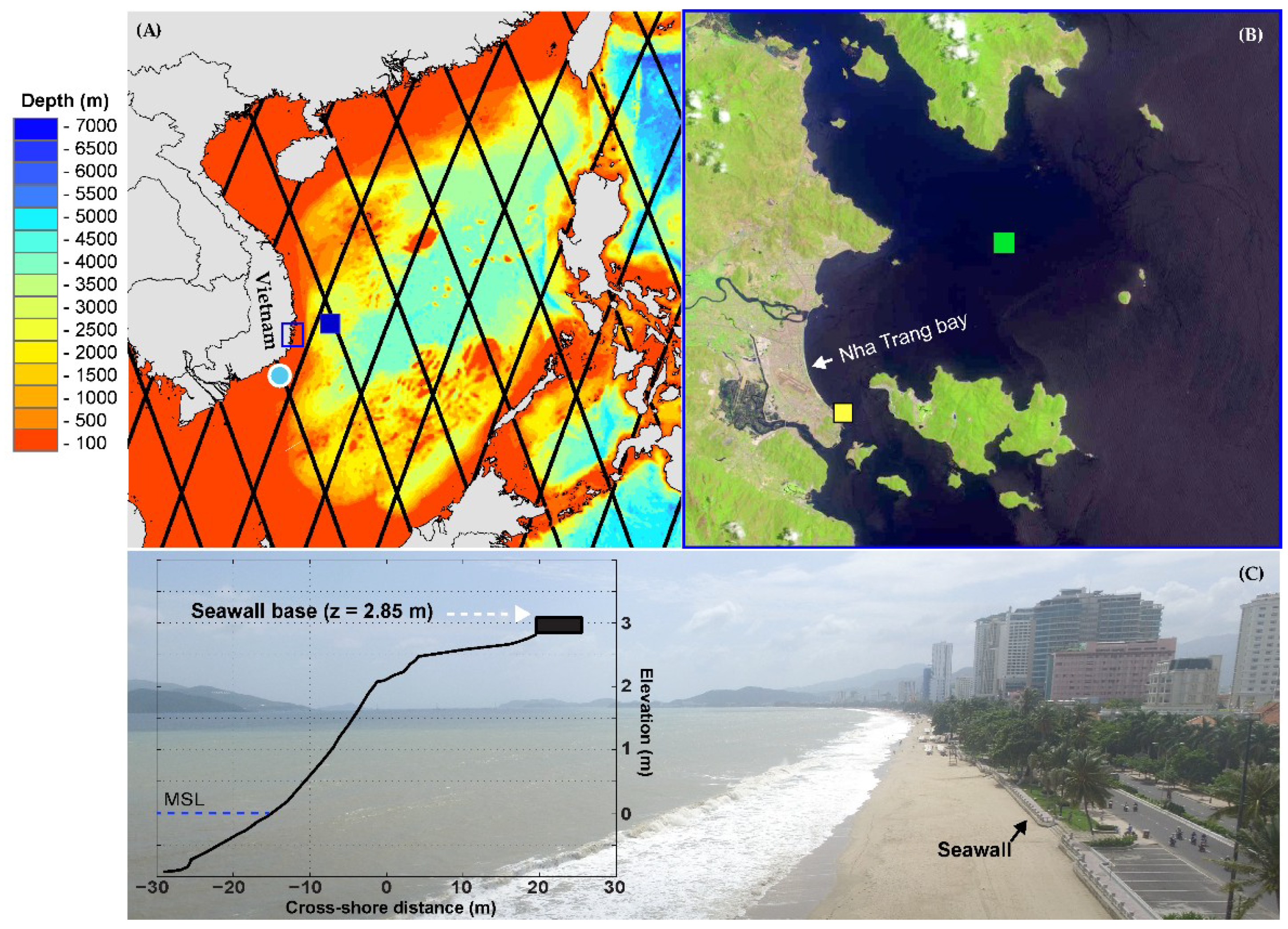
2. Study Site
3. Materials and Methods
3.1. Local Sea Level Estimation
3.2. Validation of the Datasets
4. Results
4.1. Validation
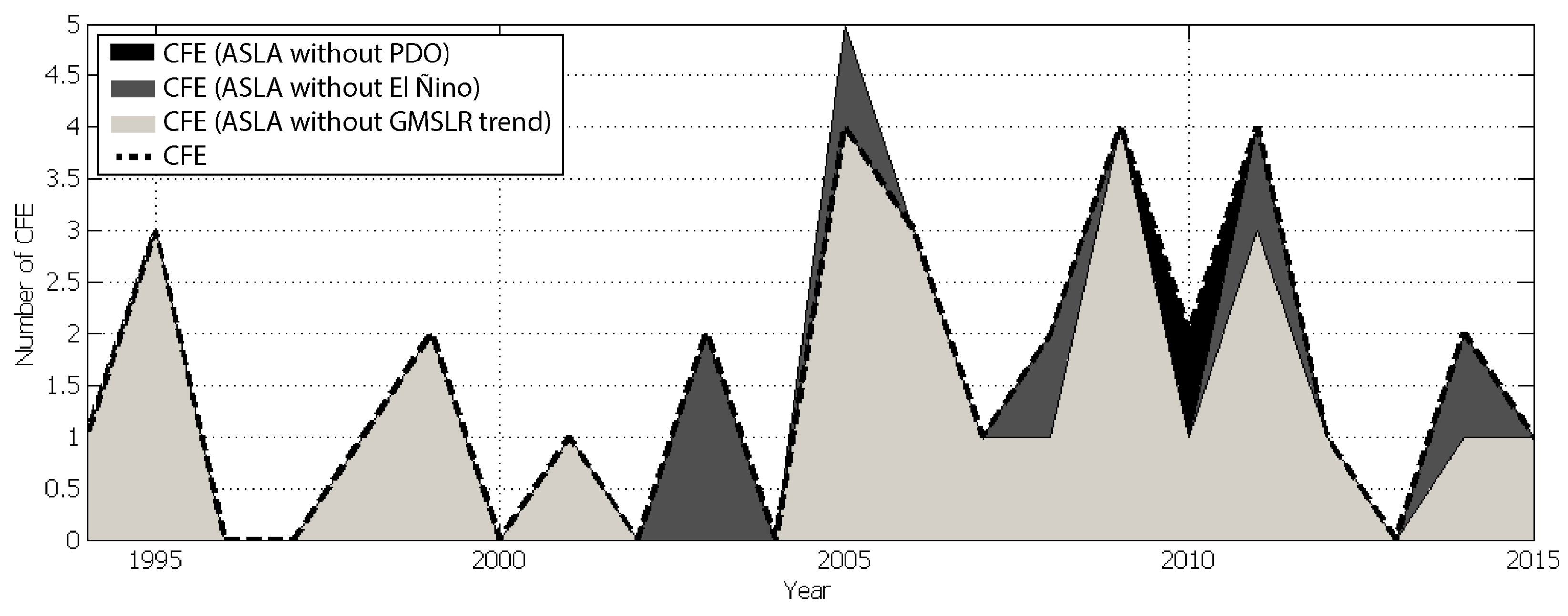
4.2. Coastal Flooding Events
4.3. Contributions of Global and Regional Climate Change to Coastal Flooding Events
5. Discussion and Conclusions
Author Contributions
Funding
Acknowledgments
Conflicts of Interest
References
- Field, C.B.; Barros, V.R.; Dokken, D.J.; Mach, K.J.; Mastrandrea, M.D.; Bilir, T.E.; Chatterjee, M.; Ebi, K.L.; Estrada, Y.O.; Genova, R.C.; et al. IPCC 2014: Climate Change 2014: Impacts, Adaptation, and Vulnerability. Part A: Global and Sectoral Aspects; Contribution of Working Group II to the Fifth Assessment Report of the Intergovernmental Panel on Climate Change; Cambridge University Press: Cambridge, UK, 2014; 1132p. [Google Scholar]
- Barros, V.R.; Field, C.B.; Dokken, D.J.; Mastrandrea, M.D.; Mach, K.J.; Bilir, T.E.; Chatterjee, M.; Ebi, K.L.; Estrada, Y.O.; Genova, R.C.; et al. IPCC 2014: Climate Change 2014: Impacts, Adaptation, and Vulnerability. Part B: Regional Aspects; Contribution of Working Group II to the Fifth Assessment Report of the Intergovernmental Panel on Climate Change; Cambridge University Press: Cambridge, UK, 2014; 688p. [Google Scholar]
- Kopp, R.E.; Horton, R.M.; Little, C.M.; Mitrovica, J.X.; Oppenheimer, M.; Rasmussen, D.J.; Strauss, B.H.; Tebaldi, C. Probabilistic 21st and 22nd century sea-level projections at a global network of tide-gauge sites. Earth Future 2014, 2, 383–406. [Google Scholar] [CrossRef]
- DeConto, R.M.; Pollard, D. Contribution of Antarctica to past and future sea-level rise. Nature 2016, 531, 591–597. [Google Scholar] [CrossRef] [PubMed]
- Dieng, H.N.; Cazenave, A.; Meyssignac, B.; Ablain, M. New estimate of the current rate of sea level rise from a sea level budget approach. Geophys. Res. Lett. 2017, 44, 3744–3751. [Google Scholar] [CrossRef]
- Melet, A.; Meyssignac, B.; Almar, R.; Le Gozannet, G. Under-estimated wave contribution to coastal sea-level rise. Nat. Clim. Chang. 2018, 8, 234–239. [Google Scholar] [CrossRef]
- Nicholls, R.J.; Marinova, N.; Lowe, J.A.; Brown, S.; Vellinga, P.; de Gusmão, D.; Hinkel, J.; Tol, R.S. Sea-level rise and its possible impacts given a ‘beyond 4 °C world’ in the twenty-first century. Philos. Trans. R. Soc. A 2011, 369, 161–181. [Google Scholar] [CrossRef] [PubMed]
- Barnard, P.L.; Short, A.D.; Harley, M.D.; Splinter, K.D.; Vitousek, S.; Turner, I.L.; Allan, J.; Banno, M.; Bryan, K.R.; Doria, A.; et al. Coastal vulnerability across the Pacific dominated by El Niño/Southern Oscillation. Nat. Geosci. 2015, 8, 801–807. [Google Scholar] [CrossRef]
- Harley, M.D.; Turner, I.; Kinsela, M.A.; Middleton, J.H.; Mumford, J.; Splinter, K.D.; Phillips, M.S.; Simmons, J.A.; Hanslow, D.J.; Short, A.D. Extreme coastal erosion enhanced by anomalous extratropical storm wave direction. Sci. Rep. 2017, 7, 6033. [Google Scholar] [CrossRef] [PubMed]
- Almeida, L.P.; Vousdoukas, M.I.; Ferreira, O.; Rodrigues, B.A.; Matias, A. Thresholds for storm impacts on an exposed sandy coastal area in southern Portugal. Geomorphology 2012, 143–144, 3–12. [Google Scholar] [CrossRef]
- Melet, A.; Almar, R.; Meyssignac, B. What dominates sea level at the coast: A case study for the Gulf of Guinea. Ocean Dyn. 2016, 66, 623–636. [Google Scholar] [CrossRef]
- Serafin, K.A.; Ruggiero, P.; Stockdon, H.F. The relative contribution of waves, tides, and non-tidal residuals to extreme total water levels on US West Coast sandy beaches. Geophys. Res. Lett. 2017, 44, 1839–1847. [Google Scholar] [CrossRef]
- Wadey, M.P.; Brown, J.M.; Haigh, I.D.; Dolphin, T.; Wisse, P. Assessment and comparison of extreme sea levels and waves during the 2013/14 storm season in two UK coastal regions. Nat. Hazards Earth Syst. 2015, 15, 2209–2225. [Google Scholar] [CrossRef]
- Dangendorf, S.; Arns, A.; Pinto, J.G.; Ludwing, P.; Jensen, J. The exceptional influence of storm ‘Xaver’ on design water levels in the German Bight. Environ. Res. Lett. 2016, 11, 054001. [Google Scholar] [CrossRef]
- Wahl, T.; Haigh, I.D.; Nicholls, R.J.; Arns, A.; Dangendorf, S.; Hinkel, J.; Slangen, A.B.A. Understanding extreme sea levels for broad-scale coastal impact and adaptation analysis. Nat. Commun. 2017, 8, 16075. [Google Scholar] [CrossRef] [PubMed]
- Vitousek, S.; Barnard, P.L.; Fletcher, C.H.; Frazer, N.; Erikson, L.; Storlazzi, C.D. Doubling of coastal flooding frequency within decades due to sea-level rise. Sci. Rep. 2017, 7, 1399. [Google Scholar] [CrossRef] [PubMed]
- Thoang, T.T.; Giao, P.H. Subsurface characterization and prediction of land subsidence for HCM City, Vietnam. Eng. Geol. 2015, 199, 107–124. [Google Scholar] [CrossRef]
- Almar, R.; Marchesiello, P.; Almeida, L.P.; Hai, T.D.; Tanaka, H.; Viet, N.T. Shoreline response to a sequence of typhoon and monsoon events. Water 2017, 9, 364. [Google Scholar] [CrossRef]
- Cheng, X.; Xie, S.P.; Du, Y.; Wang, J.; Chen, X.; Wang, J. Interannual-to-decadal variability and trends of sea level in the South China Sea. Clim. Dyn. 2016, 46, 3113–3126. [Google Scholar] [CrossRef]
- Thuan, D.H.; Binh, L.T.; Viet, N.T.; Hanh, D.K.; Almar, R.; Marchesiello, P. Typhoon Impact and Recovery from Continuous Video Monitoring: A Case Study from Nha Trang Beach, Vietnam. J. Coast. Res. 2016, 75, 263–267. [Google Scholar] [CrossRef]
- Birol, F.; Fuller, N.; Lyard, F.; Cancet, M.; Nino, F.; Delebecque, C.; Fleury, S.; Toublanc, F.; Melet, A.; Saraceno, M.; Léger, F. Coastal Applications from Nadir Altimetry: Example of the X-TRACK Regional Products. Adv. Space Res. 2017, 59, 936–953. [Google Scholar] [CrossRef]
- Carrère, L.; Lyard, F.; Cancet, M.; Guillot, A.; Roblou, L. FES2012: A new global tidal model taking advantage of nearly 20-years of altimetry. In Proceedings of the 20 Years of Progress in Radar Altimetry Symposium, Venice, Italy, 24–29 September 2012. [Google Scholar]
- Stockdon, H.F.; Holman, R.A.; Howd, P.A.; Sallenger, A.H. Empirical parameterization of setup, swash, and runup. Coast. Eng. 2006, 53, 576–588. [Google Scholar] [CrossRef]
- Dee, D.P.; Uppala, S.M.; Simmons, A.J.; Berrisford, P.; Poli, P.; Kobayashi, S.; Andrae, U.; Balmaseda, M.A.; Balsamo, G.; Bauer, P.; et al. The ERA-Interim reanalysis: Configuration and performance of the data assimilation system. Q. J. R. Meteorol. Soc. 2011, 137, 553–597. [Google Scholar] [CrossRef]
- Almeida, L.P.; Almar, R.; Blenkinsopp, C.; Martins, K.; Benshila, R.; Daly, C. Swash dynamics of a sandy beach with low tide terrace. In Proceedings of the Coastal Dynamics Conference, Helsingør, Denmark, 12–16 June 2017; p. 143. [Google Scholar]
- Islam, T.; Srivastava, P.K.; Rico-Ramirez, M.A.; Dai, Q.; Gupta, M.; Singh, S.K. Tracking a tropical cyclone through WRF–ARW simulation and sensitivity of model physics. Nat. Hazards 2015, 76, 1473–1495. [Google Scholar] [CrossRef]
- Zhang, X.; Church, J.A. Sea level trends, interannual and decadal variability in the Pacific Ocean. Geophys. Res. Lett. 2012, 39, L21701. [Google Scholar] [CrossRef]
- Potty, J.; Oo, S.M.; Raju, P.V.S.; Mohanty, U.C. Performance of nested WRF model in typhoon simulations over West Pacific and South China Sea. Nat. Hazards 2012, 63, 1451–1470. [Google Scholar] [CrossRef]
- Osuri, K.K.; Mohanty, U.C.; Routray, A.; Kulkarni, M.A.; Mohapatra, M. Customization of WRF-ARW model with physical parameterization schemes for the simulation of tropical cyclones over North Indian Ocean. Nat. Hazards 2012, 63, 1337–1359. [Google Scholar] [CrossRef]
- Qu, T.; Kim, Y.Y.; Yaremchuk, M.; Tozuka, T.; Ishida, A.; Yamagata, T. Can Luzon Strait transport play a role in conveying the impact of ENSO to the South China Sea? J. Clim. 2004, 17, 3644–3657. [Google Scholar] [CrossRef]
- Qu, T.; Du, Y.; Sasaki, H. South China Sea through flow: A heat and freshwater conveyor. Geophys. Res. Lett. 2006, 33, L23617. [Google Scholar] [CrossRef]
- Cheng, X.; Qi, Y. Trends of sea level variations in the South China Sea from merged altimetry data. Glob. Planet. Chang. 2007, 57, 371–382. [Google Scholar] [CrossRef]
- Du, Y.; Qu, T. Three inflow pathways of the Indonesian through flow as seen from the simple ocean data assimilation. Dyn. Atmos. Oceans 2010, 50, 233–256. [Google Scholar] [CrossRef]
- Li, L.; Xu, J.; Cai, R. Trends of sea level rise in the South China Sea during the 1990s: An altimetry result. Chin. Sci. Bull. 2002, 47, 582–585. [Google Scholar] [CrossRef]
- Fang, G.; Chen, H.; Wei, Z.; Wang, Y.; Wang, X.; Li, C. Trends and interannual variability of the South China Sea surface winds, surface height, and surface temperature in the recent decade. J. Geophys. Res. 2006, 111, C11S16. [Google Scholar] [CrossRef]
- Peng, D.; Palanisamy, H.; Cazenave, A.; Meyssignac, B. Interannual sea level variations in the South China Sea Over 1950–2009. Mar. Geod. 2013, 36, 164–182. [Google Scholar] [CrossRef]


| Components | Number of CFEs |
|---|---|
| NTR + AT + R | 35 |
| NTR + AT | 0 |
| NTR + R | 5 |
| AT + R | 16 |
© 2018 by the authors. Licensee MDPI, Basel, Switzerland. This article is an open access article distributed under the terms and conditions of the Creative Commons Attribution (CC BY) license (http://creativecommons.org/licenses/by/4.0/).
Share and Cite
Melo de Almeida, L.P.; Almar, R.; Meyssignac, B.; Viet, N.T. Contributions to Coastal Flooding Events in Southeast of Vietnam and their link with Global Mean Sea Level Rise. Geosciences 2018, 8, 437. https://doi.org/10.3390/geosciences8120437
Melo de Almeida LP, Almar R, Meyssignac B, Viet NT. Contributions to Coastal Flooding Events in Southeast of Vietnam and their link with Global Mean Sea Level Rise. Geosciences. 2018; 8(12):437. https://doi.org/10.3390/geosciences8120437
Chicago/Turabian StyleMelo de Almeida, Luis Pedro, Rafael Almar, Benoit Meyssignac, and Nguyen Trung Viet. 2018. "Contributions to Coastal Flooding Events in Southeast of Vietnam and their link with Global Mean Sea Level Rise" Geosciences 8, no. 12: 437. https://doi.org/10.3390/geosciences8120437
APA StyleMelo de Almeida, L. P., Almar, R., Meyssignac, B., & Viet, N. T. (2018). Contributions to Coastal Flooding Events in Southeast of Vietnam and their link with Global Mean Sea Level Rise. Geosciences, 8(12), 437. https://doi.org/10.3390/geosciences8120437