Article

Mud Flow Reconstruction by Means of Physical Erosion Modeling, High-Resolution Radar-Based Precipitation Data, and UAV Monitoring

1
Soil and Water Conservation Unit, Technical University Bergakademie Freiberg, Agricolastraße 22, 09599 Freiberg, Germany
2
Geocoptix, Max-Planck-Straße 6, 54296 Trier, Germany
3
Deutscher Wetterdienst, Abteilung Agrarmeteorologie, Kärrnerstraße 68, 04288 Leipzig, Germany
4
Thüringer Landesanstalt für Landwirtschaft, Referat 420 Acker- und Pflanzenbau, Naumburger Straße 98, 07743 Jena, Germany
*
Author to whom correspondence should be addressed.
Geosciences 2018, 8(11), 427; https://doi.org/10.3390/geosciences8110427
Submission received: 31 July 2018 / Revised: 3 October 2018 / Accepted: 14 November 2018 / Published: 21 November 2018
(This article belongs to the Special Issue Mechanics of Erosion: Process Response to Change)

Abstract

:
Storm events and accompanying heavy rain endanger the silty soils of the fertile and intensively-used agricultural landscape of the Saxon loess province in the European loess belt. In late spring 2016, persistent weather conditions with repeated and numerous storm events triggered flash floods, landslides, and mud flows, and caused severe devastation to infrastructure and settlements throughout Germany. In Saxony, the rail service between Germany and the Czech Republic was disrupted twice because of two mud flows within eight days. This interdisciplinary study aims to reconstruct the two mud flows by means of high-resolution physical erosion modeling, high-resolution, radar-based precipitation data, and Unmanned Aerial Vehicle monitoring. Therefore, high-resolution, radar-based precipitation data products are used to assess the two storm events which triggered the mud flows in this unmonitored area. Subsequently, these data are used as meteorological input for the soil erosion model EROSION 3D to reconstruct and predict mud flows in the form of erosion risk maps. Finally, the model results are qualitatively validated by orthophotos generated from images from Unmanned Aerial Vehicle monitoring and Structure from Motion Photogrammetry. High-resolution, radar-based precipitation data reveal heavy to extreme storm events for both days. Erosion risk maps show erosion und deposition patterns and source areas as in reality, depending on the radar-based precipitation product. Consequently, reconstruction of the mud flows by these interdisciplinary methods is possible. Therefore, the development of an early warning system for soil erosion in agricultural landscapes by means of E 3D and high-resolution, radar-based precipitation forecasting data is certainly conceivable.

1. Introduction

Storm events and accompanying heavy rain endanger the fertile and fragile landscape of the Saxon loess province in the European loess belt and other loess deposits worldwide. During cultivation periods of bare soil surfaces, the silty soils can easily be eroded by water and wind due to their tendency towards soil surface sealing. Beside the primary impact of soil loss and decreasing soil fertility in the field, erosion can also cause significant off-site effects. Eroded sediments from agricultural land can enter downhill located settlements and infrastructure as mud flows and cause damage there.
In late spring 2016, the macro-atmospheric condition called “low-pressure system middle Europe” dominated weather conditions in Germany [1]. This persistent weather condition was characterized by repeated and numerous storm events and accompanying heavy rain. They triggered flash floods, landslides, and mud flows, and caused severe devastation to infrastructure and settlements throughout Germany [1,2].
In Saxony, a federal state in Germany, the rail service between Germany and the Czech Republic was disrupted twice due to two mud flows within eight days. On the evening on 23 May and in the afternoon on 31 May 2016, storm events occurred over the surrounding areas of the long-distance stretch between Dresden and Prague. As a result of the evening storm event and the triggered mud flow, a freight train ran into the dirt covering the tracks near the railway station Schmilka-Hirschmühle and derailed. Fortunately, nobody was injured, but material damage was reported [3]. Eight days later, the same location was affected by another mud flow due to the afternoon storm and accompanying heavy rain. The line had to be closed once again [4].
The German Meteorological Service (DWD) defines heavy rain as large amounts of precipitation per time unit. By definition, it mostly falls from convective clouds, and can lead to rapidly rising water levels, flooding, and often, to soil erosion [5]. With radar rainfall data, the spatial distribution of precipitation becomes possible for the first time. These radar-based precipitation data in high spatial and temporal resolution also help to detect individual storm cells and accompanying heavy rain, as well as their intensity, size, and location [6].
The effects of heavy rain have been modeled by means of radar-based precipitation data. Yu et al. [7] and Yu et al. [8] utilized a hydrologic model for runoff generation and flow routing, as well as for a real-time flood forecasting system for urban catchments. Bronstert et al. [2] investigated the flash flood of Braunsbach, Baden-Wuerttemberg, which happened during the same persistent weather condition as the aforementioned mud flows. With the help of radar-based precipitation and rain gauge data of the DWD, the flash flood was meteorologically and hydrologically analyzed.
This study aims to utilize the radar-based precipitation data of the DWD for soil erosion modeling. In soil erosion studies, the soil erosion model EROSION 3D (E 3D) is used to predict soil erosion by water in case of extreme precipitation events. The process- and physically- based model simulates the sub-processes of soil erosion by water in catchment areas. As a computer-aided and grid-based model, it is also compatible with Geographic Information Systems (GIS) [9]. Moreover, E 3D has been applied in numerous catchment areas [10,11,12,13,14,15,16,17,18,19,20,21,22]. Recent publications also deal with the generation of erosion risk maps for Saxony [20,21,23]. Depending on the resolution of the input Digital Terrain Model (DTM), these maps can be of high resolution.
The overall objective of this interdisciplinary study was to examine the feasibility of mud flow reconstruction by means of high-resolution radar-based precipitation data, high-resolution physical erosion modeling, and Structure from Motion (SfM) Photogrammetry. High-resolution, radar-based precipitation data of the DWD were used to assess the precipitation situation of the two storm events, which triggered the mud flows. Two different 5-min radar-based precipitation datasets were assessed, which is more suitable in cases of storm events and accompanying heavy rain. These radar-based precipitation data were also used as input data for the soil erosion model E 3D to reconstruct and predict mud flows. Using orthophotos generated from images taken by an Unmanned Aerial Vehicle (UAV) and by SfM Photogrammetry, the mud flows were qualitatively validated.

2. Materials and Methods
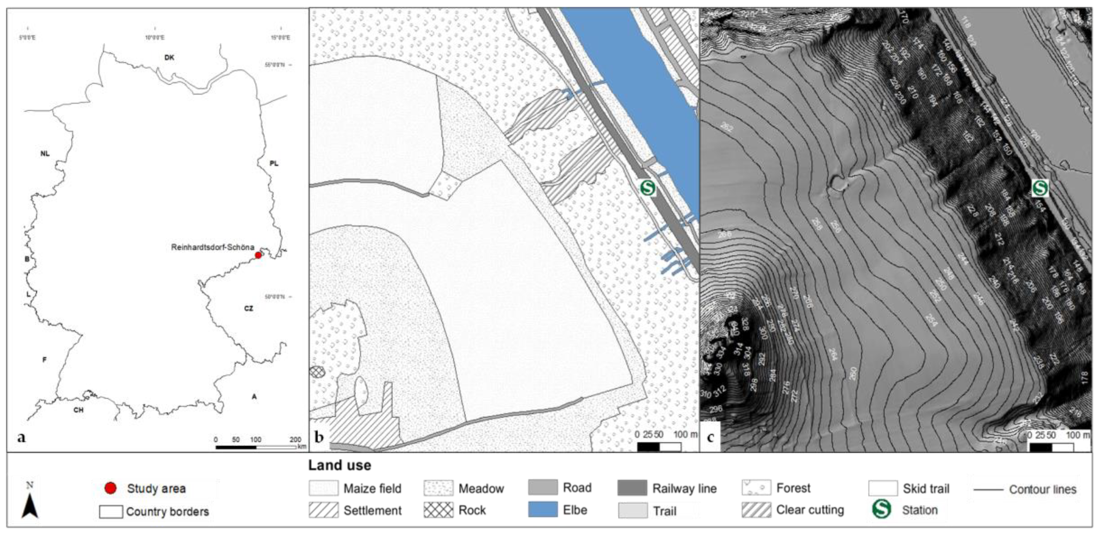
2.1. Study Area

The study area is situated near Reinhardtsdorf-Schöna within Saxony, Germany, in the immediate vicinity of the Czech border (Figure 1a). It covers an area of almost 1 km2, and is located in the Elbe Sandstone Mountains. The mean annual rainfall is around 700 mm, and the mean annual temperature lies between 7 and 8 °C. Furthermore, it is characterized by different land uses: agriculture, meadows, forests, settlements, infrastructure, and the river Elbe (Figure 1b). Belonging to the soil region of mountainous and hilly regions with high sandstone amounts, the soil textures of the study area are comprised of particular clayey silt (maize field) and pure sand (forest). The soil type of the fields is a loess Luvisol, while that of the forest is classified as a Podzol [24]. Additionally, the forest of the study area was affected by clear cutting and associated skid trails at that time (Figure 1b).

2.2. High-Resolution Radar-Based Precipitation Data

2.2.1. Data Description

The term RADOLAN is abbreviated from the German RADar-OnLine-ANeichung, meaning Radar Online Adjustment. With the RADOLAN procedure, the DWD offers a wide range of real time, high-resolution, radar-based precipitation products in different temporal resolutions and processing steps [26]. The procedure combines the advantages of quantitative radar data by the radar network of the DWD, and terrestrial rain gauge data by the common rain gauge network of the DWD and the federal states of Germany. Every five minutes, the weather radars record the reflected signals of rain and snow from higher layers of the atmosphere [27]. With these reflected and recorded signals of the so-called hydrometeors, the radar reflectivity factor Z can be determined. To determine the precipitation height, Z is converted into the precipitation intensity R via the so-called Z-R-relationship. Thus, radar measures the precipitation remotely and indirectly [6]. Though these quantitative radar data provide the spatial distribution of precipitation, their quality for water management tasks is unsatisfactory. Therefore, the measurements of fallen precipitation measured at rain gauge stations are used to adjust the quantitative radar data. During RADOLAN, this adjustment happens operationally every hour [27].
The RADOLAN products comprise high-resolution radar-based precipitation amounts from 5-min time steps ranging over one hour to 30 days and having a spatial resolution of 1 km2. Before the hourly adjustment due to rain gauge data, the quantitative 5-min radar data pass through different processing steps due to influences of the radar signal. The different processing steps are the correction of orographic attenuation, the application of a variable Z-R-relationship, quantitative compositing of the 17 weather radar sites in Germany, and additional radar sites of the neighboring countries, statistical clutter suppression, smoothing, and pre-adjustment [27].
By means of the two quantitative, high-resolution, radar-based precipitation products, RY and RZ, the overall objective of the present study will be fulfilled. Although these products are unadjusted by rain gauge data, these products pass the processing steps correction of orographic attenuation and application of a variable Z-R-relationship. Furthermore, these products contain quantitative data on precipitation in mm/5 min, and are available after two minutes [26]. Additionally, RY is quality-tested by the correction of further radar errors [28]. Both radar-based precipitation products can be applied for quantitative monitoring and visualization of precipitation and climatologic analysis of rainfall [6]. Thereby, small-scale and short-lived storm events and their quantitative and spatial distribution in time intervals of five minutes can be observed.

2.2.2. Data Preparation and Analysis

RZ- and RY-products were provided for this study by the DWD. These two and the other radar-based precipitation products of the DWD are stored in the RADOLAN Binary Data Format. These data format cannot be easily read by external users without the appropriate software application. One of these applications is Wradlib. Wradlib is an open source library for weather radar data processing. It is written in the free programming language, Python. Wradlib assists the user in the steps of processing radar data. In particular, these can be the reading of common data formats, converting reflectivity to precipitation intensity, georeferencing, and visualizing the radar data [29].
By means of Wradlib, the two 5-min radar products RZ and RY could be read, prepared, converted into another format, and finally, exported for subsequent work steps. One of the next steps was the visualization of the two storm events for the defined area of Saxony, and not for the whole of Germany. Therefore, a Python script was written which fulfilled this requirement. After converting the radar-based precipitation data into ASCII format, they could be visualized in the open source GIS QGIS [30]. Using another Python script, which included the reading of precipitation intensities for a defined area, these intensities were automatically written to a csv-file. The latter serves not only as input data for E 3D, but also provides the actual precipitation intensities for analytical purposes. Therefore, it is possible to assess the intensity of the evening and afternoon storm events in five- and ten-minute, and one-hour increments (Table 1). Thus, heavy rain is characterized by a precipitation amount greater than or equal to 10 mm in one hour and 1.7 mm in ten minutes, respectively [5].

2.2.3. Data Comparison with Rain Gauge Data

RZ and RY were not adjusted with rain gauge data, but were compared with each other. In addition, radar-based precipitation amounts are quantitative precipitation estimation products, as they are measured remotely and indirectly.
The nearest rain gauge station to the study area is Lichtenhain-Mittelndorf, and was used for the comparison. It is a precipitation monitoring station of the DWD and situated in Mittelndorf, a place near Reinhardtsdorf-Schöna, but on the eastern side of the Elbe river. Data of the rain gauge station are freely available via the Open Data Server of the DWD [31].

2.3. High-Resolution Physical Erosion Modeling Using EROSION 3D

2.3.1. Modeling Approach and Components

Schmidt [32] developed the theoretical principles of E 3D. Initially, these principles were implemented in the model EROSION 2D [10,33], the slope profile version for the prediction of soil erosion. In the following years, von Werner developed the catchment area version EROSION 3D [34].
Infiltration was modeled using the Green-Ampt approach [35]. The infiltration rate was calculated with the Darcy equation [10]. A flow path model derived from a DTM was used for the spatial distribution of the surface runoff [36]. Particle detachment and transport were simulated by the momentum flux approach by Schmidt [10,32,33]. E 3D is well validated [37,38,39,40,41] and documented [9].
E 3D consists of two main components: the pre-processing and the processing component. The pre-processing component performs the digital relief analysis with its GIS module in order to calculate the runoff and its movement in the terrain. The processing component executes the actual simulation with the sub-processes of soil erosion. The latter are as follows: infiltration of precipitation (Green-Ampt approach), runoff generation, detachment of soil particles from the ground (momentum flux approach), particle and associated pollutant transport, as well as deposition, depending on the transport capacity of the surface runoff and the enrichment of soil particles along the transport path (Figure 2) [9].

2.3.2. Input and Output Data

Figure 2 demonstrates the individual program sequences of E 3D and the input and output data requirements. The input data sets include a DTM for the relief parameter, a digital soil and a digital land use map for the soil and land use parameter, as well as precipitation data for the meteorological parameter. The geometric basis for the grid-based E 3D is a square grid having a maximum resolution of 1 m. Thus, depending on the input DTM, high-resolution erosion risk and deposition maps can be created [9].
The precipitation data input file requires a resolution of ten minutes or higher. E 3D is not only able to simulate discrete precipitation events, but also a number of successive events by means of the long-term simulation module [9].
The soil and land use data set requires additional data and processing steps including a land use grid, the physical soil properties in form of a table with the corresponding land use IDs of the land use grid, as well as a lookup table. The lookup table consists of the land use ID and the corresponding soil parameter data set key of the table [9].
E 3D requires seven soil parameters for the table of the soil and land use data set: (1) bulk density [kg/m3]; (2) organic carbon [% by weight]; (3) initial soil moisture [% by volume]; (4) hydraulic roughness [s/m1/3]; (5) resistance to erosion [N/m2]; (6) cover [%], and (7) soil texture [% by weight] [9]. Furthermore, E 3D offers an additional factor, the so-called skinfactor [–], to correct the infiltration ability [10]. Cultivation related effects on infiltration, surface runoff, and particle detachment are considered by the parameters skinfactor, resistance to erosion, and hydraulic roughness.
An extensive data basis for the parameterization of the soil parameter table was created by 116 rainfall simulations on erosion-prone slopes during the “soil erosion measurement program for Saxony” [37,38,39,40,41], which is documented in the parameter catalogue of Saxony [43]. Here, the corresponding soil parameter can be determined depending on the land use, type of use, cultivation, and soil texture. Additionally, this data basis is included in the data base of 726 rainfall simulation experiments for surface runoff from arable land, which is freely available [44]. Furthermore, a software for the automated parameterization of the soil parameters exists, which is called DPROC, and uses the data of the parameter catalogue. With current Digital Landscape Models (DLMs), it is possible to automatically assign the soil parameters of a given landscape extract via the DPROC [45,46].

2.3.3. Model Parameterization

This study utilizes a DTM with a resolution of 2 m [47] for the generation of the relief data set. The radar-based precipitation intensities of the RZ- and RY-products in mm/5 min and with a precipitation duration of 3 h serve as meteorological input data for E 3D. Thereby, one RADOLAN-grid cell with an area of 1 km2 represents the precipitation intensity on the study area.
The land use grid of this study was generated by the union and raster converting of the digital soil map 1:50,000 [24], and the digitalized land use by means of the WMS digital orthophotos RGB [48] in ArcGIS [49]. The DPROC was not used due to the missing current DLM.
The relevant soil parameters were determined according to the parameter catalogue. Thereby, soil parameters of missing anthropogenic land uses like roads and settlements were adapted following Arévalo [50].
At the time in which the mud flows happened, the forest was affected by clear cutting and associated skid trails (Figure 1b). Usually, the soil parameters of a forest on a pure, sandy soil would be parameterized as follows (Table 2):
By the inspection of the study area, it became obvious that the pure sandy soil was riddled with pebbles and stones. Therefore, the bulk density was increased to 1400 kg/m3 (Table 3). The parameter catalogue did not comprise soil parameters for clear cuttings and skid trails. Following Zemke [51], who investigated runoff and soil erosion on forest roads, the bulk densities of these areas were increased, and their hydraulic roughnesses decreased (Table 3). The complete parameterization of the physical soil properties of the study area is available in the Supplementary Materials.

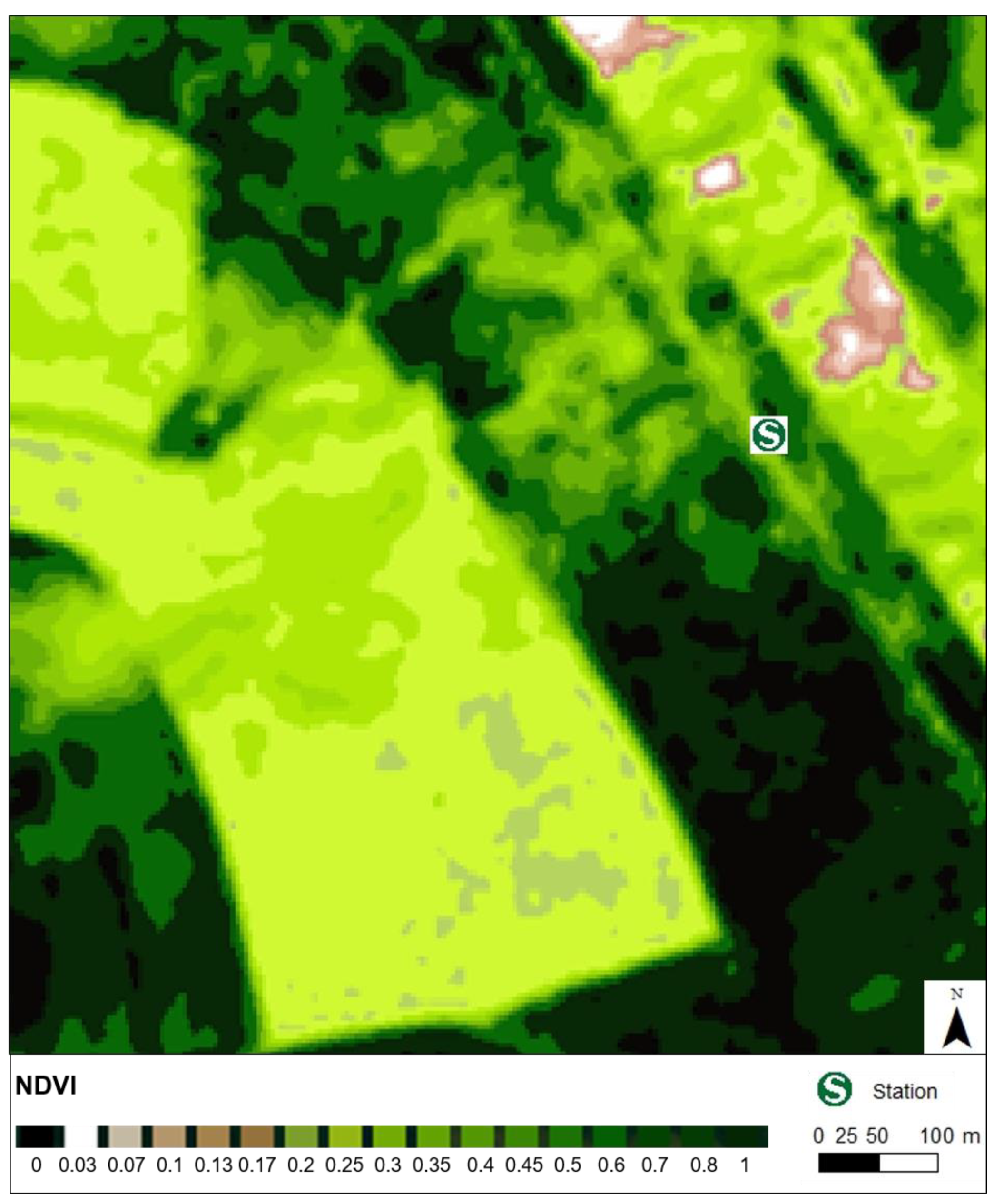
2.3.4. Derivation of Land Cover from NDVI Products of Land Viewer

The NDVI product of the Land Viewer [52] was used to derive the land cover for the E 3D soil parameter ‘cover’. It was used to identify sparsely-vegetated fields with bare soil surfaces, which are prone to soil erosion.
NDVI is the Normalized Difference Vegetation Index, and is calculated using the Red band (with its information about chlorophyll absorption) and the Near Infrared band (with its relatively high reflectance of vegetation) of a satellite scene. As a result, an image is created revealing the relative biomass. The NDVI is not only used to map desert encroachment and to monitor drought, but also to monitor agricultural production [52].
Land Viewer is a web interface for satellite imagery of the company EOS. The user has free access to remote sensing imagery of the satellites Landsat 7, Landsat 8, Sentinel-2, Sentinel-1, and other remote sensing data. The images are readily available and processed on-the-fly, as well as in real-time [52].
Figure 3 contains the NDVI for the study area on 29 May 2016 that was acquired from Sentinel-2. With a bright green color indicating a NDVI of 0.25, it reveals a sparsely vegetated maize field. The light green and cauliflower-like structure over the maize field, the dark green forest, and the white Elbe are clouds. Consequently, the E 3D soil parameter ‘cover’ can be estimated at 15%.

2.3.5. Soil Moisture Modeling Using METVER

Modeling soil moisture is required since it is subject to temporal and spatial fluctuations due to weather and soil conditions [53]. This study utilizes METVER to simulate the E 3D soil parameter ‘initial soil moisture’ using the mean value of the soil moisture of the nearest three weather stations around Reinhardtsdorf-Schöna (Lichtenhain-Mittelndorf, Dresden-Hosterwitz and Dippoldiswalde-Reinberg).
METVER is a water balance model for use in agricultural landscapes, and predicts daily soil moisture. It has been developed by Müller and Müller [54,55,56], and is used and updated by the DWD. METVER is based on the determination of real and potential evapotranspiration by the method of Turc [57] and its modification after Wendling et al. [58]. As the soil moisture depends on land use, soil texture, and type of use, it requires several parameters. The meteorological data for sunshine duration, precipitation, and daily mean temperature, and the soil data for soil texture, soil capacity, and permanent wilting point, as well as land use are used to model the soil moisture [59,60].

2.3.6. Comparison of Model Results with Undisturbed Forest Model Results

As the parameterization of anthropogenic land use, such as clear cutting and skid trails, requires a comprehensible adaption of all soil parameters, and taking into account the fact that forest was disturbed at that time, it is useful to compare the model results including clear cutting with undisturbed forest model results.

2.4. UAV Monitoring

For this study, E 3D was validated qualitatively by comparing UAV orthophotos to high-resolution, simulated erosion and deposition patterns and source areas. The UAV flight was performed on 1 June 2016 with the two mud flows in advance. Thereby, the last mud flow happens one day behind.

2.4.1. UAV and Digital Camera

The study area was mapped with the UAV ‘Phantom 2′ (quadrocopter) from DJI Innovations (Shenzhen, China). The UAV is equipped with a ‘PowerShot S100′ from Canon (Tokyo, Japan) with image stabilization, allowing it to maintain the stability and quality while acquiring photos. About 700 overlapping images were utilized to guarantee the cover of the sediment source and deposition areas, as well as the erosion patterns.

2.4.2. SfM Photogrammetry

The resulting overlapping images were processed with SfM Photogrammetry and multi-view dense matching methods in Agisoft PhotoScan [61], resulting in a dense point cloud. In a further work step, an orthophoto was generated from the dense point cloud, representing eroded parts of the study area.
Small data gaps in the orthophoto are due to missing images which occur because of the rapidly changing relief in the slope area and associated challenge of flying over the trees.

3. Results

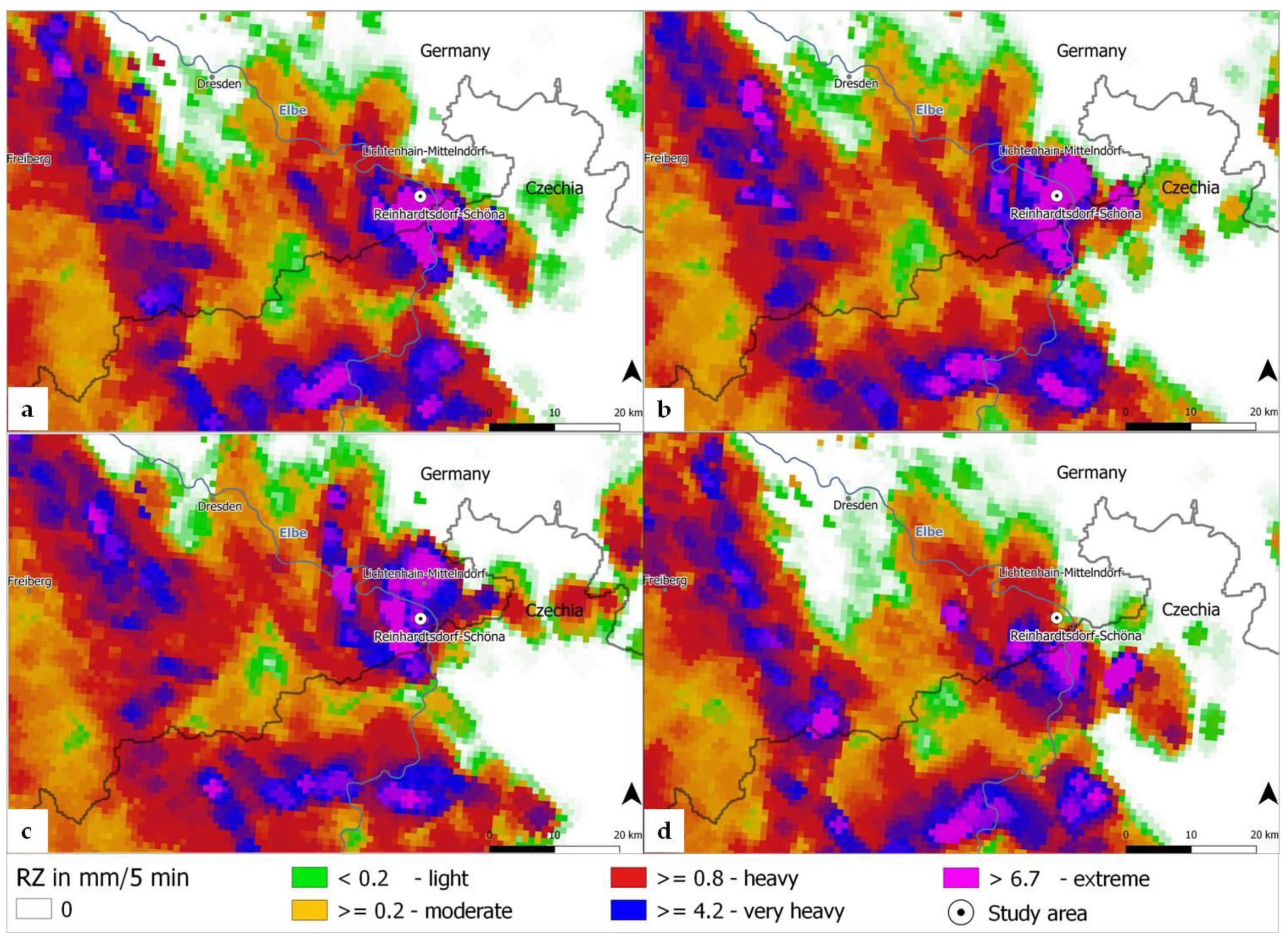
3.1. High-Resolution Radar Precipitation Data

RZ and RY products were analyzed concerning their precipitation intensity and spatial distribution for the two storm events on 23 May 2016 and on 31 May 2016. Each product will be described and then compared and discussed later. The obviously lower amount of precipitation and intensity of the RY-product will be discussed later.

3.1.1. The RZ-Product

The selected storm events were categorized according to their precipitation intensity (Table 1). Figure 4 illustrates the distribution of selected storm events for the RZ-product in 5-min time steps.
A moderate precipitation intensity began on 23 May 2016 at 6:20 p.m. and was characterized by heavy intensity at 6:40 p.m., culminating in an extreme value of 12.6 mm/5 min at 7:20 p.m. (Figure 4a). Subsequently, precipitation declined to heavy and moderate intensities before another heavy event at 8:00 p.m. Within one hour, 33 mm of rain had fallen, from which 16.6 mm fell within ten minutes. Consequently, this storm event was categorized as a heavy rain event, which was characterized by a precipitation amount of more than 10 mm in one hour. Regarding its intensity of 16.6 mm within ten minutes, the storm event contained extreme amounts of precipitation.
Figure 4b illustrates a different rainfall situation for the RZ-product on 31 May 2016. Between 1:30 and 2:00 p.m. a small precipitation cell passed Reinhardtsdorf-Schöna with a precipitation amount of 11.7 mm resulting in a heavy intensity. Then, 15 min later, another storm cell passed the same area with higher amounts of precipitation and intensity, where 54.2 mm of rain fell within one hour and 14.7 mm within ten minutes. This corresponded to a high intensity event over one hour, and an extreme event over ten minutes.
Figure 5 contains a part of the storm event on 23 May 2016 from 7:10 p.m. to 7:25 p.m. One of the precipitation cells of the northwestward-moving thunderstorm passed the study area. The most intense 15 min of the thunderstorm are mapped showing, very heavy and extreme intensity.
The heavy and very heavy storm events of 31 May 2016 developed over the Elbe Sandstone Mountains and moved westward in the early afternoon [1]. Figure 6 demonstrates the route and the most intensive 15 min of the selected storm event. The northwestward-moving storm event was much smaller than the thunderstorm on 23 May 2016, but with longer lasting, very heavy to extreme precipitation intensities.

3.1.2. The RY-Product

The RY-product on 23 May 2016 (Figure 7a) yielded precipitation amounts of 13.9 mm over one hour, from which 9.2 mm fell within ten minutes and was classified as a heavy rain event. Moreover, this storm event exceeded the very heavy threshold of 8.3 mm/10 min. In addition, the value of 7.8 mm/5 min at 7:20 p.m. exceeded the limit for classification as extreme precipitation intensity.
The pre-event on 31 May 2016 lasted from 1:35 to 1:55 p.m. and resulted in a precipitation amount of 1.6 mm (Figure 7b). Another precipitation cell passed the same area with higher amounts 20 min later. In this second event, 23.8 mm fell within one hour and 9.0 mm within ten minutes, respectively. Considering the amount of precipitation falling within one hour, the event was characterized as heavy rain. In its most intensive ten minutes, it achieved the intensity of a very heavy rain event.
As shown in Figure 8, the northwestward-moving thunderstorm cell of the 23 May 2016 evening storm was small-scale and short-lived, and heavy to extreme in its intensity.
Figure 9 contains the most intense 15 min of the afternoon storm on 31 May 2016. The second event started with heavy intensities, before the storm event culminated in a very heavy intensity at 2:30 p.m (5.4 mm/5 min). Then, the precipitation intensity declined to heavy rain.

3.1.3. Data Comparison with Rain Gauge Data

By comparing radar precipitation data (Figure 4 and Figure 7) with rain gauge data, it became obvious that the storm events began later at the rain gauge station (Figure 10). On the one hand, the thunderstorm cells approached Lichtenhain-Mittelndorf later on both days. On the other hand, the maximum value of the storm event at Lichtenhain-Mittelndorf was indicated earlier in the radar precipitation data than at the rain gauge station. The RZ- and RY-products demonstrate the maximum value at Lichtenhain-Mittelndorf on 23 May 2016 at 7:30 and on 31 May 2016 at 2:45 p.m. There was a time difference of 10 to 20 min between radar and rain gauge data (Figure 4 and Figure 7). This time shifting will be discussed later. In addition, the pre-event on 31 May 2016 was missing in the rain gauge data because this little heavy thunderstorm cell did not reach Lichtenhain-Mittelndorf.
By comparing the precipitation intensities of the rainfall data (Table 4), rain gauge data are more similar to the RZ-product on 23 May 2016. The second storm event on 31 May 2016 contained nearly the same values between the RZ-product and rain gauge data for the 10-min precipitation intensities, but not for the hourly intensity. By looking at the precipitation situation, the difference between the hourly intensities becomes comprehensible. The thunderstorm passed Lichtenhain-Mittelndorf faster than it did the study area. This, in turn, led to lower precipitation amounts in one hour at the rain gauge station. But the precipitation intensities of the most intensive ten minutes remained the same for both locations. As a result, the RZ-product should provide more reliable precipitation data in case of a storm event.

3.2. High-Resolution Physical Erosion Modeling Using EROSION 3D

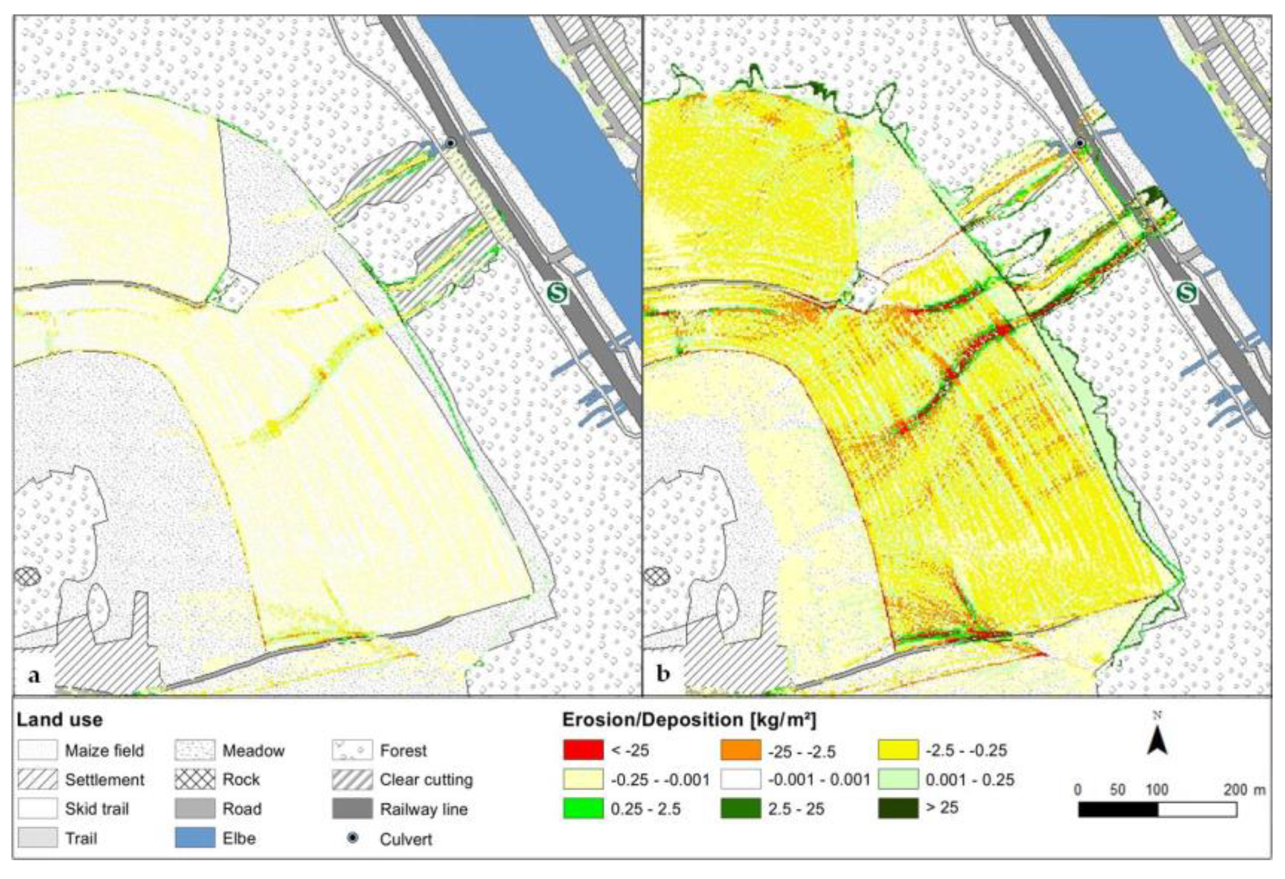
3.2.1. Soil Erosion Modeling for 23 May 2016

Figure 11 illustrates the erosion risk map as sediment budget maps of the study area created by the soil erosion model E 3D for RY- and RZ-products on 23 May 2016. On the underlying land use, yellow to red colors indicate loss, and light green to dark green colors indicate deposition of the soil particles. Most of the soil erosion for the RY-product occurred on skid trails and the clear cutting area. Only a very small part reaches the railway line in the valley. The modeled soil deposition amounts to 65.6 kg/m2. Besides the areas south of the maize field and the little erosion alongside the road in the middle of the picture, no further erosion occurred (Figure 11a).
Results are different using the RZ-product (Figure 11b). Following the bottom contour lines of the relief on the maize field and forming erosion rills (Figure 1c), soil particles were eroded and transported due to the higher precipitation amount of the RZ-product. They passed the small forest in the middle of the study area and the narrow meadow strip in front of the large forest. Downgradient eroded sediments entered the forest and followed the skid trails and the surrounding clear cutting areas. Besides the southeast skid trail, the particle loaded water sought its own way by passing the bottom contour line of the slope and eroding particles and gravel from the shallow soils of the forest. These evolved erosion rills are visible on the erosion risk map. Part of the sediment load was deposited at the margin of the bottom contour line. As the remaining load reached the railway line, it partly deposited over a distance of 160 m between the two skid trails, amounting to 386.0 kg/m2.
Figure 11b reveals another soil particle deposit on the railway line, at the end of the northeast skid trail to the northwest. At this point, a culvert drains excessive water. However, E 3D cannot model culverts, and consequently, the model incorrectly resulted in deposition on the railway line. Finally, E 3D models another soil deposit on the meadows behind the railway line in the direction of the Elbe. This fact will be described later.

3.2.2. Soil Erosion Modeling for 31 May 2016

Soil erosion occurred to a much greater extent for the RY-Product on 31 May 2016 (Figure 12a) than on 23 May 2016. Almost the complete maize field was affected by erosion. Eroded soil particles were deposited as a linear feature on the meadow in front of the forest and in the clear cutting area. 63.8 kg/m2 soil were deposited on the railway line, approximately the same amount as on 23 May 2016.
The RZ-product for 31 May 2016 shows the heaviest soil erosion and deposition patterns and amounts due to more than two times the precipitation amount (54.2 mm/h) of the RY-product (23.8 mm/h) (Figure 12b). Additionally, the RZ precipitation amount was more than one and a half times higher than that of 23 May 2016 (33.3 mm/h). Furthermore, the RZ model results demonstrated the same reproduction of the erosion rills on the maize field and in the clear cutting areas as for the other simulated cases.
The deposition on the railway tracks amounted to 757.4 kg/m2. On the railway tracks themselves, another soil erosion event occurred in the model results. Due to the fact that with higher resolution of the DTM, the whole runoff is only routed over one grid cell, the excess sediment laden water can erode again. Afterward, it deposited on the meadows in the direction of the Elbe.

3.2.3. Comparison of Model Results with Undisturbed Forest Model Results

Figure 13 illustrates the model results for all storm events and radar-based precipitation data for an undisturbed forest. Almost all erosion maps show the known soil erosion and deposition patterns for the maize field, but no notable erosion in the forest. Eroded soil particles were deposited on the meadow and in the forest.
However, Figure 13d revealed another situation. A portion of the runoff passed the bottom contour line of the slope and deposited 381.0 kg/m2 on the railway line. That is nearly half the amount of the disturbed forest for the same precipitation amount on the same day. As a result, this model result indicated that the mud flow would have happened even in case of an undisturbed forest.

3.3. UAV Monitoring

Figure 14 demonstrates the high-resolution simulated erosion and deposition patterns and source areas for the RZ-product on 31 May 2016 in comparison to the corresponding orthophoto.
The SfM generated orthophoto matches the main flow routes of sediment laden water on the maize field, through the small forest, the meadow, and in the forest. Moreover, the sediment source areas are visible and identifiable. Consequently, E 3D results could be satisfactorily validated in their spatial context.

4. Discussion

The analysis and visualization of the radar-based precipitation data for the evening storm on 23 May 2016 and the afternoon storm on 31 May 2016 revealed lower amounts of precipitation and intensities for the RY-product. Differences with the RZ-product were due to the quality test of the RY-product. However, by comparing radar-based precipitation data with rain gauge data, the RZ-product appeared to provide more reliable data in cases of storm events. As discussed in [6], the RZ-product provides plausible data, especially in cases of high amounts of precipitation. However, little to moderate precipitation are overestimated by RZ. Therefore, it is particularly suited for the analysis of extreme precipitation events. In contrast, RY is of high quality in cases of little-to-moderate precipitation. According to [62], who compared rain gauge with both 5-min radar-based precipitation data, the quality tested RY underestimated heavy rain events to a greater extent than RZ. The same publication and Einfalt and Frerk [63], as well as Peters [64], emphasized that there is a time shift between radar and rain gauge data. Radar detects the precipitation significantly earlier than the rain gauge station. Namely, this time shift is a result of different measurement heights, with the rain gauge stations being on the ground and radar aloft above ground. Therefore, the heavy rain with its consequent mud flows must have happened on 23 May around 8 p.m. and on 31 May 2016 between 2:30 and 3 p.m., as was reported for 23 May 2016 [65].
The lower precipitation amounts of the RY-product led to soil erosion almost solely in the clear cutting area on 23 May 2016. The modeled soil erosion and deposition patterns and amounts for the RZ- (23 and 31 May) and RY-products (31 May) result from higher precipitation amounts and modeled soil moisture, but differ in their intensity. After exceeding a threshold value, with increasing initial soil moisture, the soil loss increases [10].
The erosion patterns on the maize field, through the small forest, the meadow, and in the disturbed forest were reconstructed with a DTM of 2 m. However, only after adapting the soil parameters of the railway line, the clear cutting area, and the skid trails, the soil erosion in the forest and its deposition on the railway line could be achieved. Here, their bulk densities were increased and their hydraulic roughnesses were decreased. Model results indicate soil deposition on the railway between the two skid trails over a length of 160 m. In reality, the deposition was longer, up to 260 m, between the railway station and the culvert [66]. Model results with the RZ-product on 31 May 2016 indicate that a mud flow would have happened even without the parameterized clear cutting. Finally, soil erosion model results were qualitatively validated by SfM-generated orthophotos.

5. Conclusions

The modeled RZ erosion risk maps for 23 and 31 May 2016 appear to be the most representative, especially as is evidenced in the orthophoto. The distribution of the sediment deposition on the railway line was less than actual measurements, but mostly fit with reality. The erosion risk map for 31 May 2016 indicated that a mud flow would have happened even without clear cutting. Consequently, the reconstruction of mud flows by means of high-resolution real-time radar-based precipitation data, high-resolution physical erosion modeling, and SfM Photogrammetry is possible. Therefore, the simulated erosion risk maps can aid in making predictions of soil erosion. Hence, the development of an early warning system for soil erosion in agricultural lands by means of E 3D and high-resolution, radar-based precipitation forecasting data seems possible. As these radar-based precipitation forecasting data could be available up to two hours in advance, a warning is possible.
As early warning systems need an automated process chain with current data, future work should first focus on the acquisition of an actual data base like DTMs or DLMs. Furthermore, the DPROC for the automated assignment of the soil parameters has to be updated. Further research should also tackle the automated derivation of land use with the NDVI to determine the E 3D soil parameter ‘cover’. Finally, before the development of interfaces, other possible soil moisture models should be tested for the determination of the sensitive soil parameter ‘initial soil moisture’.

Supplementary Materials

The following are available online at https://www.mdpi.com/2076-3263/8/11/427/s1, Table S1: Parameterization of the study area.

Author Contributions

Conceptualization, A.K., M.S., J.S.; Methodology, A.K., M.S., P.H., F.B.; Software, P.H., A.K., M.S., S.L.; Validation, P.H., A.K., M.S., S.L.; Formal Analysis, P.H., A.K., M.S.; Investigation, P.H., A.K., M.S.; Resources, X.X.; Data Curation, X.X.; Writing—Original Draft Preparation, P.H.; Writing—Review & Editing, P.H., J.S., M.S.; Visualization, P.H.; Supervision, M.S., J.S.; Project Administration, M.S., J.S.; Funding Acquisition, A.K., J.S., M.S.

Funding

The present study was only possible due to the financial support of the European Social Fund in the Free State of Saxony (project: doctorate).

Acknowledgments

This study was only possible due to the provision of the RZ- and RY-products by Tanja Winterrath of the DWD. The authors wish to thank her and Mario Hafer of the DWD for his GIS-expertise of the RADOLAN products. Furthermore, the authors would like to thank the team of Wradlib for their instructive help with Wradlib. We want to thank the reviewers for their valuable comments on the manuscript.

Conflicts of Interest

The authors declare no conflict of interest. The funders had no role in the design of the study; in the collection, analyses, or interpretation of data; in the writing of the manuscript, and in the decision to publish the results.

Abbreviations

DLMDigital Landscape Model
DTMDigital Terrain Model
DWDgerman term, abbreviated from Deutscher Wetterdienst meaning German Meteorological Service
E 3DEROSION 3D Soil Erosion Model
GISGeographic Information System
METVERgerman term, abbreviated from METeorologisches VERdunstungsmodell, meaning meteorological evaporation model
NDVINormalized Difference Vegetation Index
RADOLANgerman term, abbreviated from RADar-OnLine-ANeichung meaning Radar Online Adjustment
SfMStructure from Motion
UAVUnmanned Aerial Vehicle

References

  1. Ziese, M.; Junghänel, T.; Becker, A. Andauernde Großwetterlage Tief Mitteleuropa Entfaltet Ihr Unwetterpotential mit Starken Gewittern und Massiven Schadensgeschehen in Deutschland. Available online: https://www.dwd.de/DE/leistungen/besondereereignisse/niederschlag/20160603_starkregen_mai-2016_medlung.pdf (accessed on 18 July 2018).
  2. Bronstert, A.; Agarwal, A.; Boessenkool, B.; Fischer, M.; Heistermann, M.; Köhn-Reich, L.; Moran, T.; Wendi, D. Die Sturzflut von Braunsbach am 29. Mai 2016—Entstehung, Ablauf und Schäden eines “Jahrhundertereignisses”. Teil 1: Meteorologische und hydrologische Analyse. The Braunsbach Flashflood of Mai 29th, 2016—Origin, Pathways and Impacts of an Extreme Hydro-Meteorological Event. Part 1: Meteorological and Hydrological Analysis. Hydrol. Wasserbewirtsch. 2017, 61, 150–162. [Google Scholar] [CrossRef]
  3. earth-chronicles.com. A Landslide Disrupted Rail Service between Dresden and Prague. Available online: http://earth-chronicles.com/natural-catastrophe/a-landslide-disrupted-rail-service-between-dresden-and-prague.html (accessed on 14 September 2016).
  4. Radio Leipzig. Unwetter Sorgt für Schäden in Sächsischer Schweiz. Available online: www.radioleipzig.de/beitrag/unwetter-sorgt-fuer-schaeden-in-saechsischer-schweiz-230485 (accessed on 23 July 2018).
  5. DWD Wetterlexikon. Available online: www.dwd.de/lexikon (accessed on 22 July 2018).
  6. DWA-Themen. Niederschlagserfassung durch Radar und Anwendung in der Wasserwirtschaft—T2/2017; Deutsche Vereinigung für Wasserwirtschaft, Abwasser und Abfall e. V.: Hennef, Germany, 2017; pp. 1–99. ISBN 978-3-88721-478-4. [Google Scholar]
  7. Yu, B.; Seed, A.; Lin, P.; Malone, T. Integration of weather radar data into a raster GIS framework for improved flood estimation. Atmos. Sci. Lett. 2005, 6, 66–70. [Google Scholar] [CrossRef] [Green Version]
  8. Yu, B.; Seed, A.; Trevithick, R.; Morris, K. Design and testing of a real-time flood forecasting system for urban catchments. Aust. J. Water Resour. 2007, 11, 161–168. [Google Scholar] [CrossRef]
  9. Von Werner, M. Erosion-3D Benutzerhandbuch; Version 3.0.; Michael von Werner: Berlin, Germany, 2002; pp. 1–82. [Google Scholar]
  10. Schmidt, J. Entwicklung und Anwendung eines physikalisch begründeten Simulationsmodells für die Erosion geneigter, landwirtschaftlicher Nutzflächen. Berliner Geographische Abhandlungen 1996, 61, 1–148. [Google Scholar]
  11. Klik, A.; Zartl, A.S.; Hebel, B.; Schmidt, J. Comparing RUSLE, EROSION 2D/3D, and WEPP Soil Loss Calculations with Four Years of Observed Data; ASAE. Annual International Meeting: Orlando, Florida, USA, 1998; ASAE No. 982055; 11p. [Google Scholar]
  12. Jetten, V.; de Roo, A.; Favis-Mortlock, D. Evaluation of field-scale and catchment-scale soil erosion models. Catena 1999, 37, 521–541. [Google Scholar] [CrossRef]
  13. Schmidt, J.; von Werner, M.; Michael, A. Application of the EROSION 3D Model to the Catsop Watershed, The Netherlands. Catena 1999, 37, 449–456. [Google Scholar] [CrossRef]
  14. Hebel, B. Validierung numerischer Erosionsmodelle in Einzelhang und Einzugsgebietsdimension. Physiogeographica Baseler Beiträge zur Physiogeographie 2003, 32, 1–181. [Google Scholar]
  15. Michael, A.; Schmidt, J.; Enke, W.; Deutschländer, T.; Malitz, G. Impact of expected increase in precipitation intensities on soil loss—Results of comparative model simulations. Catena 2005, 61, 155–164. [Google Scholar] [CrossRef]
  16. Schob, A.; Schmidt, J.; Tenholtern, R. Derivation of site-related measures to minimise soil erosion on the watershed scale in the Saxonian loess belt using the model EROSION 3D. Catena 2006, 68, 153–160. [Google Scholar] [CrossRef]
  17. Schilde, M. Modelling Soil Erosion in the Zhifanggou-Watershedon the Chinese Loess Plateau using EROSION 2/3D; TU Bergakademie Freiberg: Freiberg, Germany, 2008; 79p. [Google Scholar]
  18. Seidel, N. Untersuchung der Wirkung Verschiedener Landnutzungen auf Oberflächenabfluss und Bodenerosion mit Einem Simulationsmodell. Ph.D. Thesis, TU Bergakademie Freiberg, Freiberg, Germany, 2008. [Google Scholar]
  19. Schindewolf, M.; Schmidt, W. Validierung EROSION 3D—Prüfung und Validierung des neu entwickelten Oberflächenabflussmoduls des Modells EROSION 3D im Zusammenhang mit Maßnahmen des vorsorgenden Hochwasserschutzes auf landwirtschaftlich genutzten Flächen. Schriftenr. Landesamtes Umwelt Landwirtsch. Geol. 2009, Heft 15, 1–121. Available online: http://nbn-resolving.de/urn:nbn:de:bsz:14-ds-1244617738468-42743.
  20. Schindewolf, M. Prozessbasierte Modellierung von Erosion, Deposition und Partikelgebundenem Nähr- und Schadstofftransport in der Einzugsgebiet- und Regionalskala. Ph.D. Thesis, TU Bergakademie Freiberg, Freiberg, Germany, 2012. [Google Scholar]
  21. Steinz, A. Prozessbasierte Ermittlung des Jährlichen Partikelgebundenen Schwermetallaustrages im Einzugsgebiet der Mulde. Master’s Thesis, TU Bergakademie Freiberg, Freiberg, Germany, 2014. [Google Scholar]
  22. Starkloff, T.; Stolte, J. Applied comparison of the erosion risk models EROSION 3D and LISEM for a small catchment in Norway. Catena 2014, 118, 154–167. [Google Scholar] [CrossRef]
  23. Schindewolf, M.; Kaiser, A.; Buchholtz, A.; Schmidt, J. Development of a flash flood warning system based on real-time radar data and process-based erosion modelling. In EGU General Assembly Conference Abstracts; EGU2017-18057; EGU General Assembly: Vienna, Austria, 2017; Volume 19. [Google Scholar]
  24. BK 50 2012: Sächsisches Landesamt für Umwelt, Landwirtschaft und Geologie. Available online: https://www.umwelt.sachsen.de/umwelt/boden/27787.htm (accessed on 21 July 2018).
  25. OSM Boundaries Map 4.4.6. Wambachers-OSM.website. Available online: https://wambachers-osm.website/boundaries/ (accessed on 28 September 2018).
  26. DWD RADOLAN Produktübersicht. Available online: www.dwd.de/RADOLAN (accessed on 6 December 2017).
  27. DWD RADOLAN Kurzbeschreibung. Available online: www.dwd.de/RADOLAN (accessed on 15 December 2017).
  28. DWD. Feinspezifikation für die Erstellung eines Qualitätskomposits, Version 3.2. 2005; written communication.
  29. Heistermann, M.; Jacobi, S.; Pfaff, T. Technical Note: An open source library for processing weather radar data (wradlib). Hydrol. Earth Syst. Sci. 2013, 17, 863–871. [Google Scholar] [CrossRef]
  30. QGIS 2018. QGIS Version 3.0.1—Girona 64 bit. Available online: https://www.qgis.org (accessed on 10 April 2018).
  31. Open Data Server DWD 2018. Data Source: Deutscher Wetterdienst. Available online: https://opendata.dwd.de/ (accessed on 1 July 2018).
  32. Schmidt, J. A mathematical model to simulate rainfall erosion. In Erosion, Transport and Deposition Processes—Theories and Models; Catena Supplement; Bork, H.-R., de Ploey, J., Schick, A.P., Eds.; Catena Verlag: Cremlingen-Destedt, Germany, 1991; Volume 19, pp. 101–109. [Google Scholar]
  33. Schmidt, J. Modeling long term soil loss and landform change. In Overland Flow—Hydraulics and Erosion Mechanics; Parson, A.J., Abrahams, A.D., Eds.; UCL Press: London, UK, 1992; pp. 409–433. [Google Scholar]
  34. Von Werner, M. GIS-orientierte Methoden der Digitalen Reliefanalyse zur Modellierung von Bodenerosion in Kleinen Einzugsgebieten. Ph.D. Thesis, Freie Universität Berlin, Berlin, Germany, 1995. [Google Scholar]
  35. Green, W.H.; Ampt, G.A. Studies on soil physics. J. Agric. Sci. 1911, 4, 1–24. [Google Scholar] [CrossRef]
  36. Von Werner, M. Abschätzung des Oberflächenabflusses und der Wasserinfiltration auf landwirtschaftlich Genutzten Flächen mit Hilfe des Modells EROSION 3D; Endbericht; GeoGnostic: Berlin, Germany, 2004. [Google Scholar]
  37. LfUG. Bodenerosionsmessprogramm Sachsen—Auswertung der Beregnungsversuche 1–28 vom 04.-31.10.1993; LfUG: Freiberg, Germany, 1994. [Google Scholar]
  38. LfUG. Bodenerosionsmessprogramm Sachsen—Auswertung der Beregnungsversuche 29–49 vom 02.-12.05.1994; LfUG: Freiberg, Germany, 1994. [Google Scholar]
  39. LfUG. Bodenerosionsmessprogramm Sachsen—Auswertung der Beregnungsversuche 50–76 vom 26.09.-12.10.1994; LfUG: Freiberg, Germany, 1995. [Google Scholar]
  40. LfUG. Bodenerosionsmessprogramm Sachsen—Auswertung der Beregnungsversuche 77–94 vom 09.05.-19.5.1995; LfUG: Freiberg, Germany, 1995. [Google Scholar]
  41. LfUG. Bodenerosionsmessprogramm Sachsen—Auswertung der Beregnungsversuche 95–116 vom 03.10.-13.10.1996; LfUG: Freiberg, Germany, 1996. [Google Scholar]
  42. Kunth, F.; Kaiser, A.; Vláčilová, M.; Schindewolf, M.; Schmidt, J. Extensive Rill Erosion and Gullying on Abandoned Pit Mining Sites in Lusatia, Germany; EGU General Assembly: Vienna, Austria, 2015. [Google Scholar]
  43. Michael, A.; Schmidt, J.; Schmidt, W. Band II: Parameterkatalog Sachsen Anwendung. In EROSION 2D/3D—Ein Computermodell zur Simulation der Bodenerosion durch Wasser; Sächsische Landesanstalt für Landwirtschaft, Sächsisches Landesamt für Landwirtschaft, Umwelt und Geologie: Dresden, Freiberg, Germany, 1996; p. 121. [Google Scholar]
  44. Seibert, S.; Auerswald, K.; Fiener, P.; Disse, M.; Martin, W.; Haider, J.; Michael, A.; Gerlinger, K. Surface runoff from arable land—A homogenized data base of 726 rainfall simulation experiments. Hydrol. Earth Sys. Sci. 2011. [Google Scholar] [CrossRef]
  45. LfL. Erarbeitung der Digitalen Datengrundlage für die Anwendung von EROSION-3D auf Mesoskaliger Maßstabsebene mit Durchführung einer Erosionssimulation für das zu Bearbeitende Gebiet, Endbericht des FuE-Vorhabens der LfL; GeoGnostics: Leipzig/Berlin, Germany, 2005; pp. 1–88. [Google Scholar]
  46. Schindewolf, M.; Schmidt, J.; von Werner, M. Modeling soil erosion and resulting sediment transport into surface water courses on regional scale. ZfG Suppl. Issues 2013, 57, 157–175. [Google Scholar] [CrossRef]
  47. DTM2 2016: Staatsbetrieb Geobasisinformation und Vermessung Sachsen. Kachelnummer 4445636 und 4445638. State 2005. Available online: http://www.landesvermessung.sachsen.de/inhalt/produkte/dhm/dgm/dgm.html (accessed on 21 November 2018).
  48. WMS Digitale Orthophotos (RGB) 2015: Staatsbetrieb Geobasisinformation und Vermessung Sachsen. Available online: https://geodienste.sachsen.de/wms_geosn_dop-rgb/guest? (accessed on 21 July 2018).
  49. ArcGIS 2015. Esri ArcGIS 10.4.1 for Desktop, Version 10.4.1.5686. Available online: https://www.esri.de/support-de/produkte/startset-arcgis-104 (accessed on 21 November 2018).
  50. Arévalo, S.A. Simulation of a Local Flood Event in a Settling Area with EROSION 3D. Diploma thesis, TU Bergakademie Freiberg, Freiberg, Germany, 2009. [Google Scholar]
  51. Zemke, J. Runoff and Soil Erosion Assessment on Forest Roads Using a Small Scale Rainfall Simulator. Hydrology 2016, 3, 25. [Google Scholar] [CrossRef]
  52. Land Viewer 2018: EOS Data Analytics, Inc. Available online: https://eos.com/landviewer (accessed on 21 July 2018).
  53. Blume, H.-P.; Brümmer, G.W.; Fleige, H.; Horn, R.; Kandeler, E.; Kögel-Knabner, I.; Kretzschmar, R.; Stahr, K.; Wilke, B.-M. Scheffer/Schachtschabel Soil Science, 1st ed.; Springer: Berlin/Heidelberg, Germany, 2016. [Google Scholar]
  54. Müller, J.; Müller, G. Berechnung der Verdunstung landwirtschaftlicher Produktionsgebiete, 1. Mitteilung. Z. Meteorol. 1988, 38, 332–336. [Google Scholar]
  55. Müller, J.; Müller, G. Berechnung der Verdunstung landwirtschaftlicher Produktionsgebiete, 2. Mitteilung. Z. Meteorol. 1988, 38, 361–365. [Google Scholar]
  56. Müller, J.; Müller, G. Berechnung der Verdunstung landwirtschaftlicher Produktionsgebiete, 3. Mitteilung. Z. Meteorol. 1989, 39, 142–149. [Google Scholar]
  57. Turc, L. Évaluation des besoins en eau d’irrigation, évapotranspiration potentielle, formule simplifiée et mise à jour. Ann. Agron. 1961, 12, 13–49. [Google Scholar]
  58. Wendling, U.; Schellin, H.-G.; Thomä, M. Bereitstellung von täglichen Informationen zum Wasserhaushalt des Bodens für die Zwecke der agrarmeteorologischen Beratung. Z. Meteorol. 1991, 41, 468–475. [Google Scholar]
  59. Pilz, C. Einfluss des Klimawandels auf die Bodenfeuchte im Oberboden—Vergleichende Modellsimulationen mit dem Modell METVER auf der Grundlage von WETTREG-Klimaszenarien. Bachelor’s Thesis, TU Bergakademie Freiberg, Freiberg, Germany, 2011. [Google Scholar]
  60. Routschek, A. Auswirkungen des Klimawandels auf die Bodenerosion. Schriftenreihe des LfULG 2012, H 29, 1–138. [Google Scholar]
  61. Agisoft 2016: Agisoft PhotoScan Professional. Version 1.2.5 Build 2735 (64 bit). Agisoft LLC: St. Petersburg, Russia, 2016. Available online: http://www.agisoft.com/ (accessed on 21 November 2018).
  62. DWD RADOLAN/RADVOR-OP (Sachstand und Ausblick). Available online: https://www.dwd.de/DE/leistungen/radolan/radarniederschlagsprodukte/vortrag_2010_pdf (accessed on 15 December 2017).
  63. Einfalt, T.; Frerk, I. The challenge to estimate extreme precipitation for locations without rain gauges. In Proceedings of the ERAD 2012—The seventh European Conference on Radar in Meteorology and Hydrology, Toulouse, France, 25–29 June 2012. [Google Scholar]
  64. Peters, T. Ableitung einer Beziehung zwischen der Radarreflektivität, der Niederschlagsrate und weiteren aus Radardaten abgeleiteten Parametern unter Verwendung von Methoden der multivariaten Statistik. Ph.D. Thesis, Universität Fridericiana zu Karlsruhe (TH), Karlsruhe, Germany, 2008. [Google Scholar]
  65. n-tv.de 2016: Bahnstrecke Dresden-Prag Ist Wieder Frei. Nach Erdrutsch Blockiert. Available online: https://www.n-tv.de/panorama/Bahnstrecke-Dresden-Prag-ist-wieder-frei-article17760816.html?serv= (accessed on 23 July 2018).
  66. mdr.de 2016: Nach Erdrutsch. Bahnstrecke Dresden-Prag Wieder Frei. Available online: http://www.mdr.de/sachsen/erdrutsch-bahnstrecke-dresden-prag-gesperrt-100_zc-ecc53a13_zs-...1 (accessed on 14 September 2016).
Figure 1. The study area in (a) Germany (data basis: [25]), (b) its land use and (c) its relief.
Geosciences 08 00427 g001
Figure 2. Flow chart of EROSION 3D program sequences (changed after [42]).
Geosciences 08 00427 g002
Figure 3. The NDVI of the study area [52].
Geosciences 08 00427 g003
Figure 4. The storm events and its intensities for the RZ-product on (a) 23 and (b) 31 May 2016.
Geosciences 08 00427 g004
Figure 5. The selected storm event in 5-min time steps on 23 May 2016 from (a) 7:10 p.m., (b) 7:15 p.m., (c) 7:20 p.m. to (d) 7:25 p.m.
Geosciences 08 00427 g005
Figure 6. The selected storm event in 5-min time steps on 31 May 2016 from (a) 2:20 p.m., (b) 2:25 p.m., (c) 2:30 p.m. to (d) 2:35 p.m.
Geosciences 08 00427 g006
Figure 7. The storm event and its intensities for the RY-product on (a) 23 and (b) 31 May 2016.
Geosciences 08 00427 g007
Figure 8. The selected storm event in 5-min time steps on 23 May 2016 from (a) 7:10 p.m., (b) 7:15 p.m., (c) 7:20 p.m. to (d) 7:25 p.m.
Geosciences 08 00427 g008
Figure 9. The selected storm event in 5-min time steps on 31 May 2016 from (a) 2:20 p.m., (b) 2:25 p.m., (c) 2:30 p.m. to (d) 2:35 p.m.
Geosciences 08 00427 g009
Figure 10. The storm events and its intensities for the rain gauge data on (a) 23 and (b) 31 May 2016.
Geosciences 08 00427 g010
Figure 11. The erosion risk map with (a) RY- and (b) RZ-product for 23 May 2016.
Geosciences 08 00427 g011
Figure 12. The erosion risk map with (a) RY- and (b) RZ-product for 31 May 2016.
Geosciences 08 00427 g012
Figure 13. The erosion risk map with (a) RY- and (b) RZ-product for 23 May 2016 and for 31 May 2016 (c,d), respectively, for an undisturbed forest.
Geosciences 08 00427 g013
Figure 14. (a) The erosion risk map with the RZ-product for 31 May 2016 and (b) the UAV acquired orthophoto of the study site after the mud flows had occurred.
Geosciences 08 00427 g014
Table 1. The classification of the intensity of precipitation per time unit [5].
Intensitymm/5 min 1mm/10 minmm/h
Light<0.2<0.5<2.5
Moderate≥0.2–<0.8≥0.5–<1.7≥2.5–<10.0
Heavy≥0.8–<4.2≥1.7–<8.3≥10.0–<50.0
Very heavy≥4.2–<6.7≥8.3–<13.3≥50.0–<80.0
Extreme≥6.7≥13.3≥80.0
1 5-min intensity levels are calculated by adapting the calculation of the DWD [5].
Table 2. The parameterization of an undisturbed forest.
Land UseBulk DensityOrganic CarbonSkinfactorInitial MoistureHydraulic RoughnessErosion ResistanceCoverSoil Texture
Forest10000.98METVER 10.90.1100Pure sand
Table 3. The parameterization of a disturbed forest.
Land UseBulk DensityOrganic CarbonSkinfactorInitial MoistureHydraulic RoughnessErosion ResistanceCoverSoil Texture
Forest14000.98METVER 10.90.1100Pure sand
Skid trail18000.90.01METVER 10.020.0010Pure sand
Clear cutting17000.90.1METVER 10.10.0220Pure sand
Table 4. Comparison of the radar-based precipitation with rain gauge data.
Intensitymm/hmm/10 min
RZ 23 May 201633.316.6
RY 23 May 201613.89.2
Rain gauge 23 May 201635.520.2
RZ 31 May 201654.214.7
RY 31 May 201623.89.0
Rain gauge 31 May 201630.715.6

