Estimating Groundwater Abstractions at the Aquifer Scale Using GRACE Observations

Abstract

Groundwater monitoring requires costly in situ networks, which are difficult to maintain over long time periods, especially in countries facing economic recession such as Greece. Our work aims at providing a methodology to estimate groundwater abstractions at the aquifer scale using publicly available remotely sensed data from the NASA’s Gravity Recovery and Climate Experiment (GRACE) together with publicly available meteorological observations that serve as input variables to an Artificial Neural Network (ANN) method. The methodology was demonstrated in an alluvial aquifer in NE Greece for a 10-year period (2005–2014), where irrigation agriculture poses a serious threat to both groundwater resources and their dependent ecosystems. To generalize the developed model, an ensemble of 100 ANNs was created by the initial weight randomization approach and output was computed by averaging the output of each individual model. Scaled Root Mean Square Error and Nash–Sutcliffe coefficient were used to test the model efficiency. Both of these performance metrics indicated that monthly groundwater abstractions can be estimated efficiently and that the developed methodology offers an inexpensive substitute for in situ groundwater monitoring when in situ networks are not available or cannot operate properly.

1. Introduction

The European Water Framework Directive (WFD 2000/60/EC), requires adequate monitoring to ensure that both quality and quantity of groundwater remains within acceptable ranges and to safeguard sustainability of groundwater resources for the long-term. To avoid depletion of groundwater resources, the WFD (Article 4), requires that groundwater extraction must be limited to the proportion of natural recharge. Despite its importance as a resource that promotes and sustains life, monitoring groundwater availability and quality is usually a costly and complicated process, as it requires the construction and operation of a network of observational wells and the collection of measurements at regular time intervals. Even in the cases where such a network exists, the spatial and temporal coverage maybe inadequate or the maintenance costs cannot be accommodated resulting in poor functioning of such a network, constituting the acquired observations unreliable [1]. Even in the United States, where an active network of 850,000 observational wells operates [2], there is still need for more monitoring sites to better understand groundwater systems [1]. Additionally, the lack of observational data results in problems in the application of groundwater models, thus limiting their primary role as decision support tools [3].

Concerning groundwater use, previous work has shown that during the last fifty years, global groundwater abstractions have doubled, posing serious threats to many aquifers worldwide [4] and it is estimated that spatial and temporal availability of fresh water will change [5]. Additionally, climate change is also expected to impact groundwater resources, with anticipated effects being more severe in areas designated as “Hot Spots”, with the Mediterranean characterized as primary area to be affected [6,7]. It is therefore important to acquire as much information as possible concerning the status and fate of groundwater systems.

Advances in remote sensing, especially during the last fifty years, provide complementary techniques to in situ observations, producing data for reliable monitoring of environmental changes [8], whereas they constitute the only useful information in areas that are sparsely monitored [9,10]. As far as changes in groundwater storage are concerned, until now there is no remote sensing technique that could possibly determine them directly [3]. Temporal changes in total water storage (ΔTWS) i.e., surface water, soil water and groundwater, can be detected by gravitational measurements through NASA’s Gravity Recovery and Climate Experiment (GRACE). However, disaggregating changes of total water storage into individual hydrologic components requires availability of ground-based information or coupling with data provided by land surface models. In any case, it is widely accepted that remote sensing data can offer valuable information for groundwater storage [11] and can contribute towards improving inputs and constraints to hydrologic models [3,10].

The most popular technique provided for estimation of groundwater storage changes with remotely sensed data uses GRACE-derived total water storage anomalies. However, estimation of groundwater storage changes requires the determination directly or by hydrologic modeling the remainder of the TWS components and remove them from GRACE signal [12,13,14]. Besides the many advantages offered by the measurements provided by the GRACE mission, there are substantial problems related to the low effective spatial resolution (>150,000 km²) [11], that does not allow estimation of the high variability of various water storage components. Therefore, traditionally, GRACE data applications were limited to continental or regional scales [10,12], whereas ground-based observations should be available to allow estimation of interannual trend patterns of water storage. Recent works have started dealing with the problem of downscaling coarse GRACE observations at local scale using statistical downscaling techniques with readily available meteorological data [1,10]. Thus, it has been demonstrated that GRACE signal may be used along with local variables to predict groundwater level changes [10] or estimate groundwater storage changes [1] in local aquifer scales. Those achievements support decision-making related to water resources allocation and management, especially when monitoring networks fail to provide continuous reliable information.

In our work, we adopted the statistical downscaling approach in the form of an ANN model to estimate the groundwater withdrawals from a local aquifer in NE Greece, i.e., the Neon Sidirochorion aquifer. ANNs are widely known as robust tools to deal with non-linear problems. Compared to deterministic models, ANNs offer a major advantage as they do not require knowledge of any physical model. Furthermore, compared to traditional regression models, a major advantage of ANNs is their adaptive nature, i.e., their ability to learn and adjust model parameters from historical data [15]. Despite the explicit requirement of EU Water Framework Directive for effective control of groundwater use, there are still problems in Greece related to the implementation of regulations because of the economic costs related to an operational groundwater-monitoring network. Our methodology offers a parallel to in situ monitoring tool, or an independent procedure for situations when there is no monitoring network, that evaluates the extracted groundwater quantities of a groundwater body helping thus highlighting overexploited aquifers and improving sustainable use of water resources and compliance with EU legislation.

2. Materials and Methods

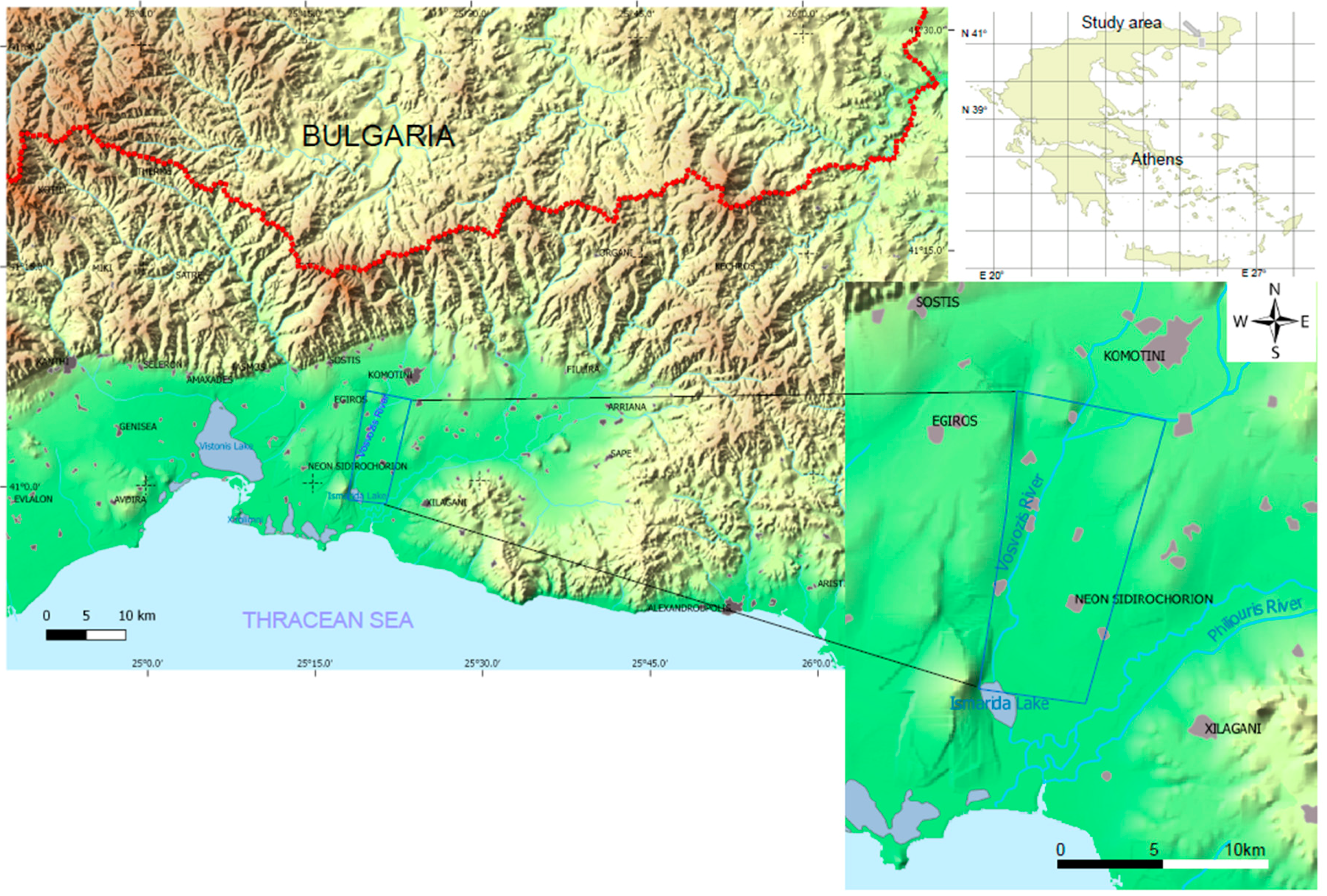
2.1. Study Area Description

The study area is located in NE Greece and comprises an alluvial aquifer known as Neon Sidirochorion aquifer (Figure 1), used for irrigation of the local corn and cotton farms during the growing period, i.e., June to August. The aquifer covers an area of 35 km² and consists of layers of sands and gravels of approximate thickness of 50–100 m. The southern part of the aquifer is hydraulically connected to Lake Ismarida, which is characterized as a groundwater dependent ecosystem. Lake Ismarida is a protected ecosystem under national and international treaties, such as the National Park of Eastern Macedonia and Thrace and the EU Natura 2000 network. Overexploitation of the aquifer causes severe groundwater level drawdown with a consequent impact on Lake Ismarida, which has rapidly depleted during the last 15-year period. The main reason for the degradation of this important ecosystem is the adjacent aquifer that constitutes a sink for lake water during irrigation period. Previous works have documented that Lake Ismarida contributes annually approximately 3.9 × 10⁶ m³ of water to Neon Sidirochorion aquifer and that there is no direct hydraulic connection of the aquifer with the sea [16]. The aquifer together with its dependent ecosystems are studied within the EU FP7 project named GENESIS (Groundwater and Dependent Ecosystems: New Scientific and Technical Basis for Assessing Climate Change and Land-use Impacts on Groundwater Systems—Grant agreement No.: 226536) and the complex interactions of surface and groundwater bodies in the area have been studied, while the need for reliable monitoring and control of groundwater abstractions has been highlighted [17,18].

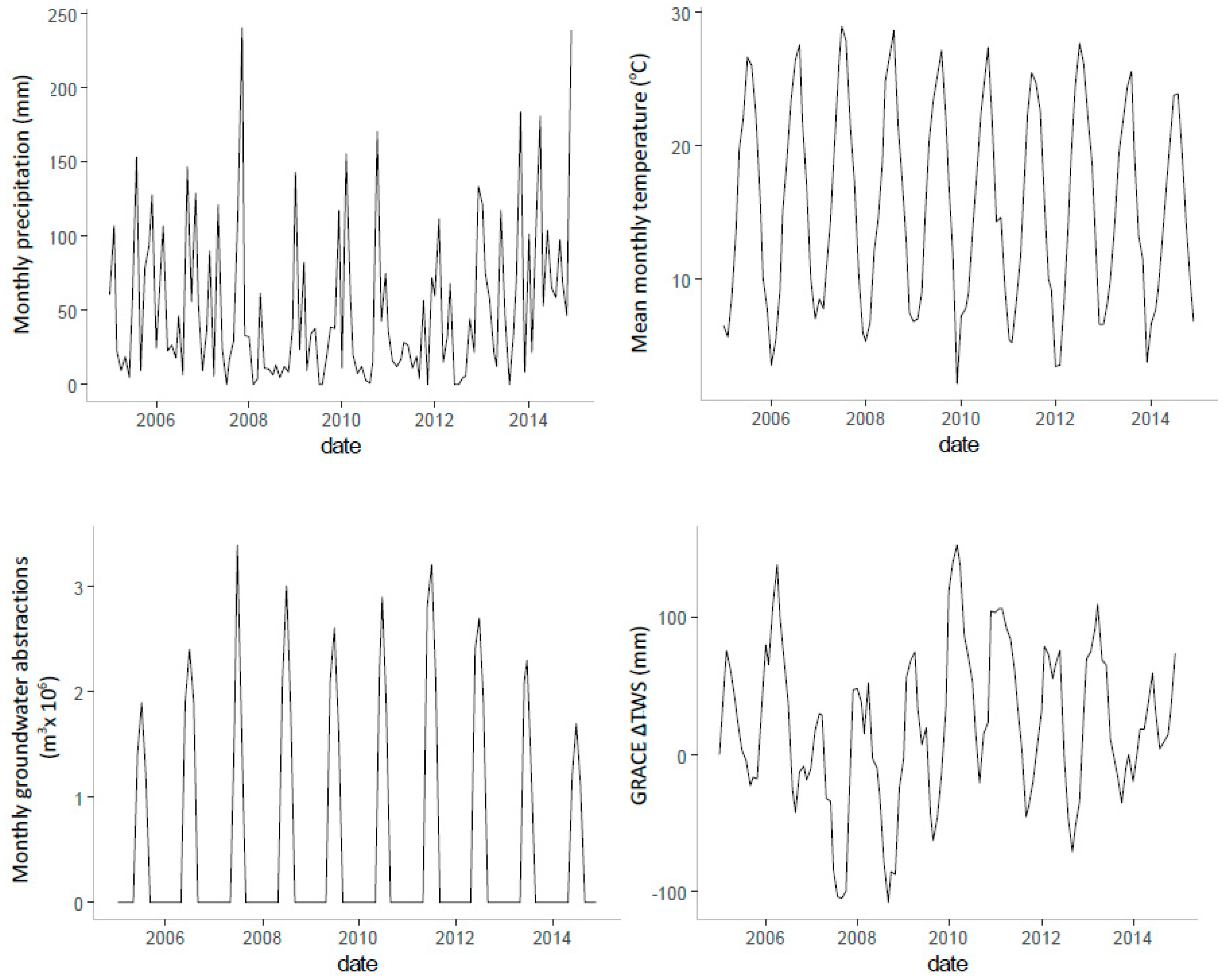
2.2. Description of the Data Set

2.2.1. GRACE Data

Gridded monthly TWS anomalies at 1° spatial resolution (approximately 110 km at the latitude of Greece) were used from GRACE mission (version 5.0 of Level 2 data) [19] with gridded gain factors and scaling factors applied according to the methodology described in [20]. GRACE is a joint mission of the US and German space agencies (NASA and DLR) launched in 2002 and consists of two identical satellites orbiting Earth, monitoring gravitational field changes. Gravity anomalies are converted into equivalent water height changes relative to a time-mean baseline [21]. Removing the atmospheric and ocean effects approximates GRACE signal with changes in terrestrial water storage (ΔTWS) [22], thus contributing a pioneering research achievement in the studies of water reservoirs over land, oceans, and ice.

GRACE data are updated regularly, and Level-2 data are produced based on the GRACE Ground System which consists of three centers: Center for Space Research (CSR) of University of Texas, GeoForschungsZentrum Potsdam (GFZ), and Jet Propulsion Laboratory (JPL). Access to data sets from all three centers is provided by the CU GRACE data portal (http://geoid.colorado.edu/grace/index.html) developed by the University of Colorado. In our work we used GRACE CSR Level 2 gridded data from 2005 to 2014.

2.2.2. Ground Observations

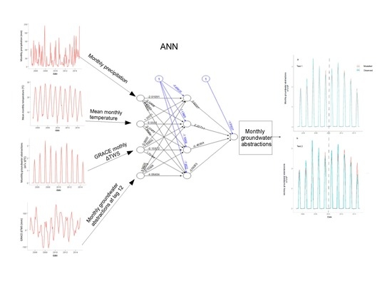
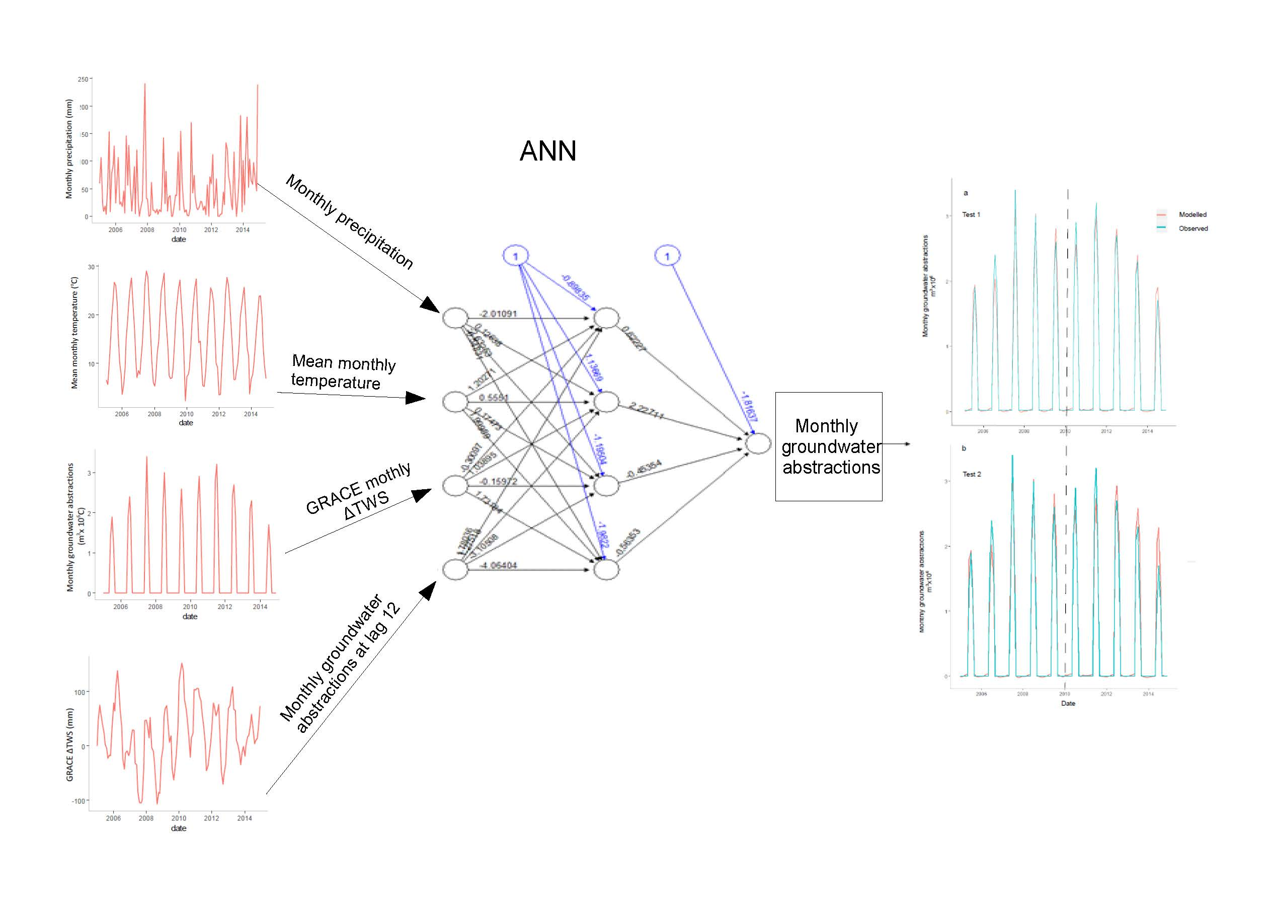
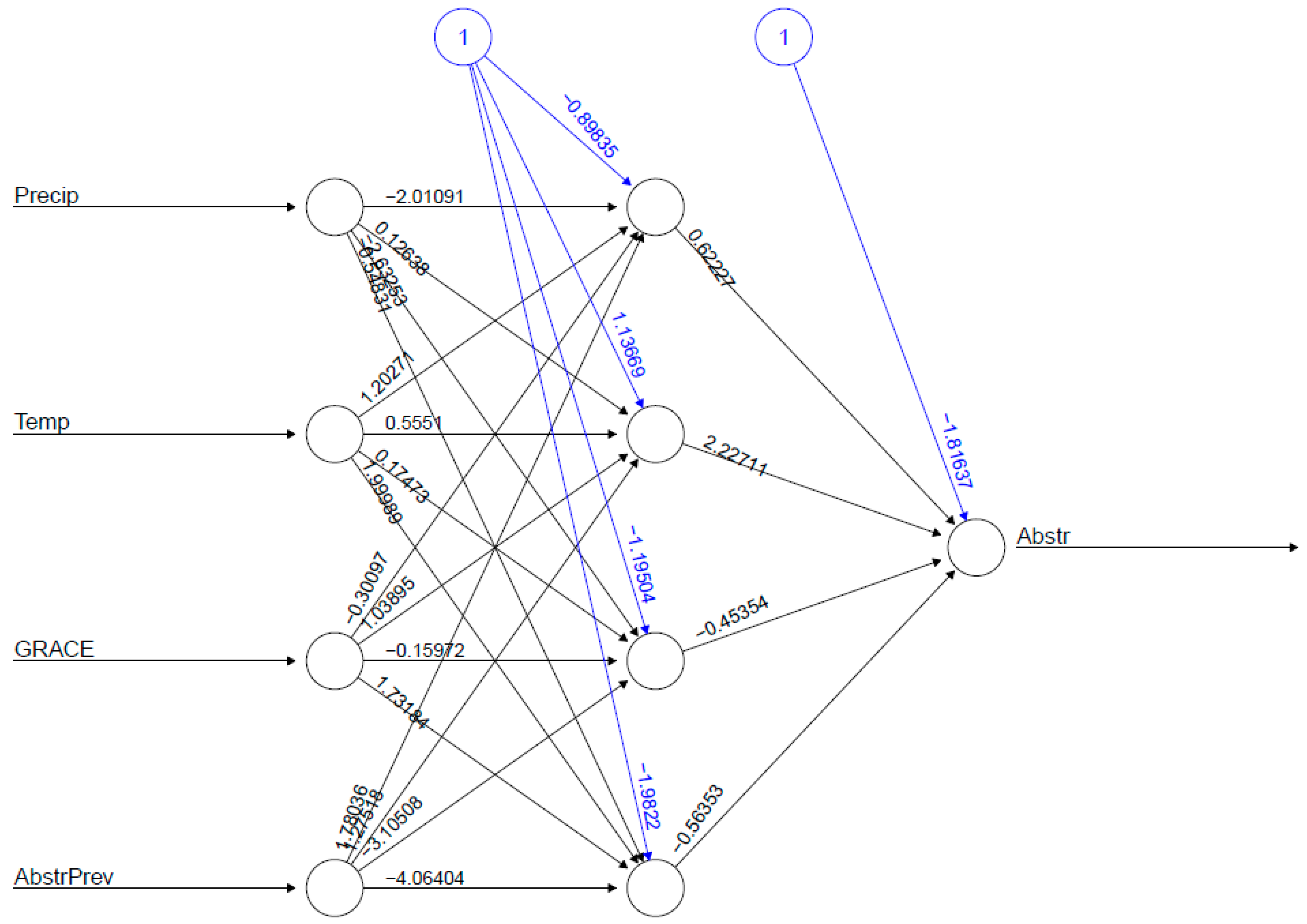
Groundwater monitoring has been implemented from early 2000 in the study aquifer and continued until 2014 within GENESIS project with groundwater level measurements in eight monitoring wells of Neon Sidirochorion aquifer. Groundwater abstractions are not recorded in the study area and consequently an implicit way to compute them needs to be determined. In our work, we used the total power consumed in the farms of the study aquifer as a proxy for monthly groundwater abstraction computations during the 10-year period from 2005 to 2014. The formula used is the one provided in [17], with total electrical power consumption per month provided by the Public Power Corporation:

$$P= \frac{Q \times H}{102 \times n}$$

(1)

In Equation (1) the total power required (P, in kW) to provide a discharge (Q in L/s) at a total pumping head (H in m) is provided. In the same equation, n corresponds to the derating which describes the pumping efficiency. Derating factors for electric and diesel motors are stated to range from 80% to 75% respectively [17,23] and 102 is a conversion factor. Groundwater head used in Equation (1) corresponds to mean value of monthly groundwater head readings in the eight observational locations.

Along with GRACE TWS anomalies, meteorological parameters from the local meteorological station of Komotini town were used as predictors in the computation process. Meteorological data comprised monthly precipitation and mean monthly temperature for the study period. Basic statistics of the data set are shown on

Table 1. Statistics of input parameters.

Parameter	Minimum Value	Maximum Value	Standard Deviation
Monthly precipitation (mm)	0.0	241.0	52.2
Mean monthly temperature (°C)	2.2	29.0	7.5
GRACE Total Water Storage anomalies—ΔTWS (mm/month)	−107.3	152.7	57.2
Monthly groundwater abstractions (m3 × 106) *	1.2	3.4	0.58

* Statistics for groundwater abstractions correspond to summer period only.

. Figure 2 presents graphs of the meteorological, groundwater abstraction and GRACE monthly ΔTWS time series. The full data set is also provided in Table S1 as Supplementary Material.

2.3. The ANN Model

Artificial neural networks (ANNs) are human-brain-inspired algorithm constructs used as machine learning models. They are also widely used in water resources modeling and time series prediction problems such as nowcasting and forecasting of groundwater levels, which have been successfully addressed using ANNs [10,24,25,26] as well as groundwater storage changes [1] and also water quality issues [15]. Within the present work a Multi-Layer Perceptron (MLP) ANN has been developed and implemented to estimate monthly groundwater quantity abstracted from Neon Sidirochorion aquifer during a ten-year period, i.e., 2005–2014. A usual problem while preparing an ANN model is the selection of input variables, which should be physically related to the target variable and at the same time they should be easily available for the computational process, as our concept was to build a model as simple as possible in terms of data requirements. Variables considered were those that are physically related to groundwater abstractions and these were precipitation and temperature, as irrigation takes place during periods of high temperature and low precipitation. GRACE monthly ΔTWS has been proved in previous works to be a useful predictor for groundwater storage changes [10,27,28] at much higher resolution compared to the footprint of GRACE [13] and it was considered as a possible predictor variable as well. We also examined whether any auto-correlative components of the target variable are present. Diagnostic tests, in the form of cross-correlation computation of external predictors, i.e., monthly precipitation, mean monthly temperature, and GRACE monthly ΔTWS with monthly groundwater abstractions were performed. This allowed assessment of the relationship of external predictors with the target variable not only at the current time but also at various time lags, i.e., whether monthly groundwater abstractions are correlated to the current value or any historical values (prior time lags) of the external variables. Estimation of auto-correlation function of the target variable at time lags was used to assess any auto-correlative components. Furthermore, various model architectures were evaluated excluding one variable in the model at a time and changing neurons of the hidden layer, so as to determine the input variable combination and hidden layer architecture that produces most satisfactory output.

When a set of input variables x is provided, the ANN estimates the target variable:

$$y=f\left(x\right) + \epsilon$$

(2)

where f is a functional mapping corresponding to a complex non-linear mathematical function that uses input data to evaluate the target variable and the associated noise (ε) in the process. A Multi-layer Perceptron (MLP) is a type of ANN that can be used to learn functional mapping [10] backpropagating the error until a predefined accuracy is reached. Even very complex nonlinear relationships between the predictor and output variables can be modeled with MLP ANNs. The structure of a typical MLP consists of one input layer, one or more hidden layers and an output layer, each with one or more neurons. Input variables are represented by neurons in the input layers, whereas one or more neurons in the output layer depict the target variable.

If M is the number of predictor variables, the set of input can be denoted as ${\left\{x_i\right\}}_{i=1}^M,$ and the K hidden layer neurons are computed as a weighted sum of predictors [10]:

$$a_k= {\displaystyle \sum }_{i=1}^M{w}_{ki}^{\left(1\right)}{x}_i+w_{k0}^{\left(1\right)}, k=1,\dots , K$$

(3)

In Equation (3), $a_k$ is a neuron in the hidden layer, ${\{w_{ki}^{\left(1\right)}\}}_{i=1}^M$ stands for the unknown weights, also known as synapse weights, with each one of the input neurons, and $w_{k0}^{\left(1\right)}$ is the term of unknown bias. Superscripts denote the layer number. A transfer function $g\left(a_k\right),$ is used to give output ($o_k)$ from neurons in the hidden layers, according to the following equation:

$$o_{k }=g\left(a_k\right), k=1,\dots , K$$

(4)

In our work, a linear transfer function is applied to convey the signal from hidden layer to the output layer:

$$y_j= {\displaystyle \sum }_{k=1}^K{w}_{jk}^{\left(2\right)}{o}_k + w_{j0}^{\left(2\right)}$$

(5)

In Equation (5) $y_j$ is the neuron of the output layer, $\{w_{jk}^{\left(2\right)}\}$ and $w_{j0}^{\left(2\right)}$ the weights and the bias term respectively, estimated within the ANN process. The number of output neurons in this work is one, although it can be greater than one, e.g., in the case of a categorical output variable. To establish a reliable ANN model, two phases are required, i.e., the training and the testing phase. The data set is thus split into two parts, one for the training and one for the testing phase, each one usually corresponding to 50% of the data set, randomly selected. In this work, because the unknown variable, i.e., monthly groundwater abstraction quantity, forms a time series, the data set is split into two consecutive periods, i.e., one for testing and one training phase. The former constitutes the period from 2005 to 2009 and the latter is taken to be the 2010–2014 period. During training, the backpropagation algorithm adjusts fitting weights in each layer until best fit of modeled to observed data is reached.

A usual problem while developing an ANN is overtraining and happens because of the complexity and non-homogeneity of data [29]. Overtraining is present when a perfect fit is found in the training data set and a substantial lower fit is observed in the testing phase. The model thus cannot be considered as general. To generalize an ANN and improve its stability, especially when sample size is small, which is a common problem in studies of water resources, an ensemble of ANNs was developed. It is well recognized that an ensemble of ANN models improves the general ability of the model compared to a single ANN model [10,30,31]. In our work, we adopted the approach of initial weight randomization to create an ensemble of 100 ANNs, as this technique has proved to be as accurate as more sophisticated ensemble generation techniques [10]. The ensemble output is computed by averaging the output of each individual model. In each model, performance in training and testing phase was calculated to ensure that overtraining is not present.

R, an open and free statistical computing software has been implemented for the whole modeling process. The Neuralnet tool [32] within R, supported the creation of the ensemble of MLP ANNs in this work.

The statistical metrics of model performance include both metrics of absolute error and goodness-of-fit, that both should be part of a complete assessment of model performance [33,34]. Thus, two criteria were used for assessing model performance at the testing phase:

(a)

Scaled Root Mean Square Error (RMSE) ranging from 0 to a large value, denoted as R*:

$$R^{*}=\frac{RMSE}{{\sigma }_o}= \frac{\sqrt{\frac{1}{n}{{\displaystyle \sum }}_{t=1}^n{\left(P_t-O_t\right)}^2} }{{\sigma }_o}$$

(6)

(b)

Nash–Sutcliffe model efficiency (NSE) ranging from −∞ to 1, [35]:

$$NSE=1-\frac{{{\displaystyle \sum }}_{t=1}^n{\left(O_t-P_t\right)}^2}{{{\displaystyle \sum }}_{t=1}^n{\left(O_t-\overline{O}\right)}^2}$$

(7)

In Equations (6) and (7) $P_t$ corresponds to prediction at month t, $O_t$ is observation at the same month, ${\sigma }_o$ is the standard deviation of observed values, whereas $\overline{O}$ is the mean of the observed values and n is the number of months at the testing phase. According to [10,36] a model is considered to have very good performance when NSE > 0.75 and R* < 0.50.

Data were scaled linearly standardizing them to a [0, 1] range, to make the process faster, as sometimes the target and predictor variables have very different ranges. First half of the time series data, i.e., 2005 to 2009, was used for training the ANN and the remainder, i.e., 2010–2014 was used for testing the developed model.

Two testing procedures were performed, i.e., Test 1 and Test 2, a first (Test 1) where the groundwater abstractions at lag 12 were used from the original groundwater abstraction time series as an input variable (Test 1) and a second (Test 2) where the groundwater abstraction at lag 12 was used from the constantly updated groundwater abstraction time series. This is achieved by feedback to the ANN every estimated monthly groundwater abstraction value, to be used as input for the rest unknown groundwater abstraction quantities. If Test 2 proves to be of acceptable accuracy, then data requirements for groundwater abstractions are minimized, since each month’s results are used as input by the time they are available.

To estimate relative importance of each variable in the developed model, the connection weight method was applied, which is proved to be robust [10,37]. According to the connection weight technique, quantification of the relative importance of input variables in an ANN, uses connection weights between input and hidden layers and between hidden and output layers in the trained network. Firstly, the input to hidden layer weights matrix IH is computed which is a K × M matrix, where K is the number of neurons in the hidden layer and M is the number of input variables. Secondly, the hidden to output layers weights vector HO, of length K, is evaluated. An element-wise product of IH and HO gives a matrix P of dimensions K × M. Summing across the rows of P produces the importance vector IV, of length K, whose elements are calculated as follows:

$$I{V}_i=\frac{\left|I{V}_i\right|}{{{\displaystyle \sum }}_{i=1}^K\left|I{V}_i\right|}$$

(8)

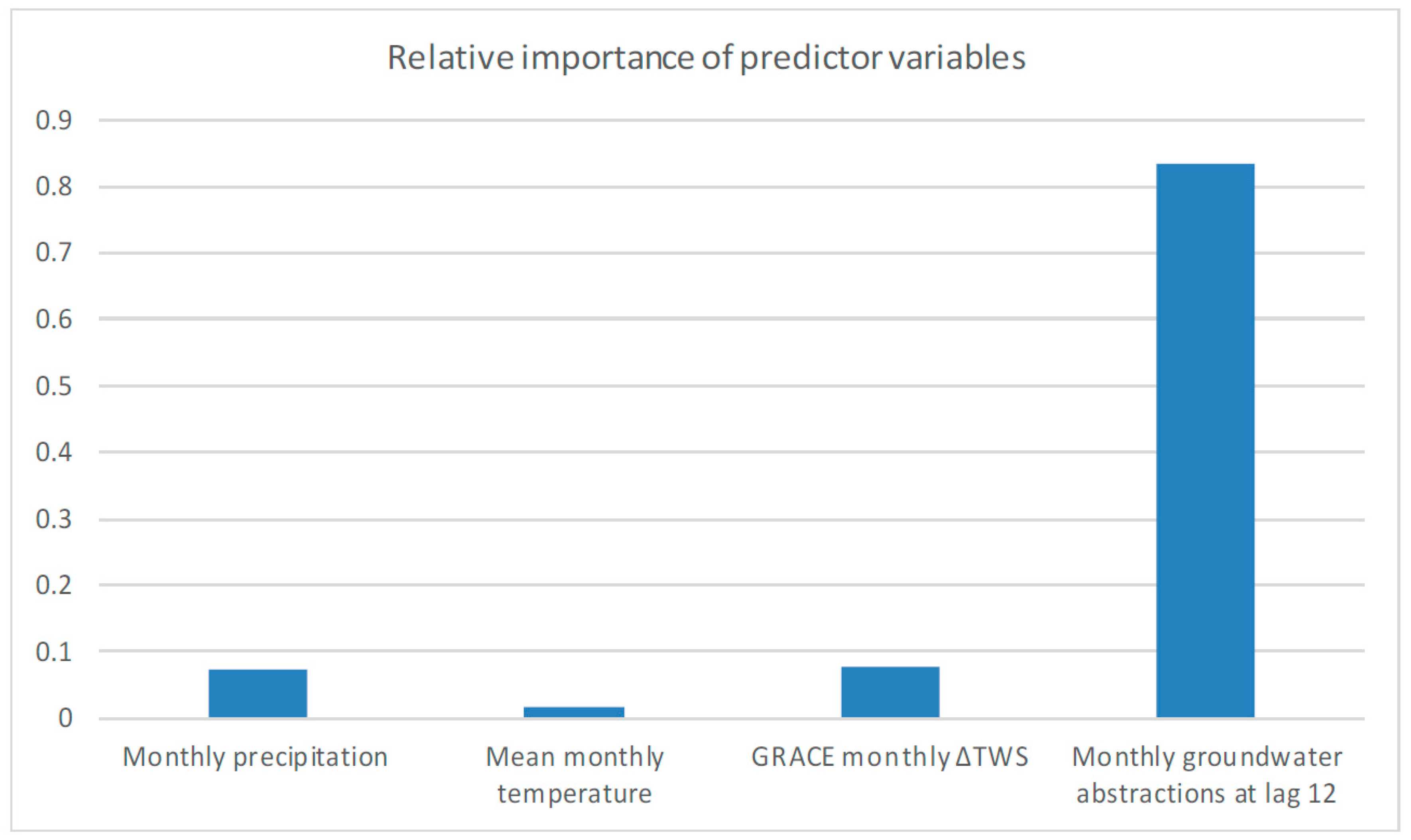
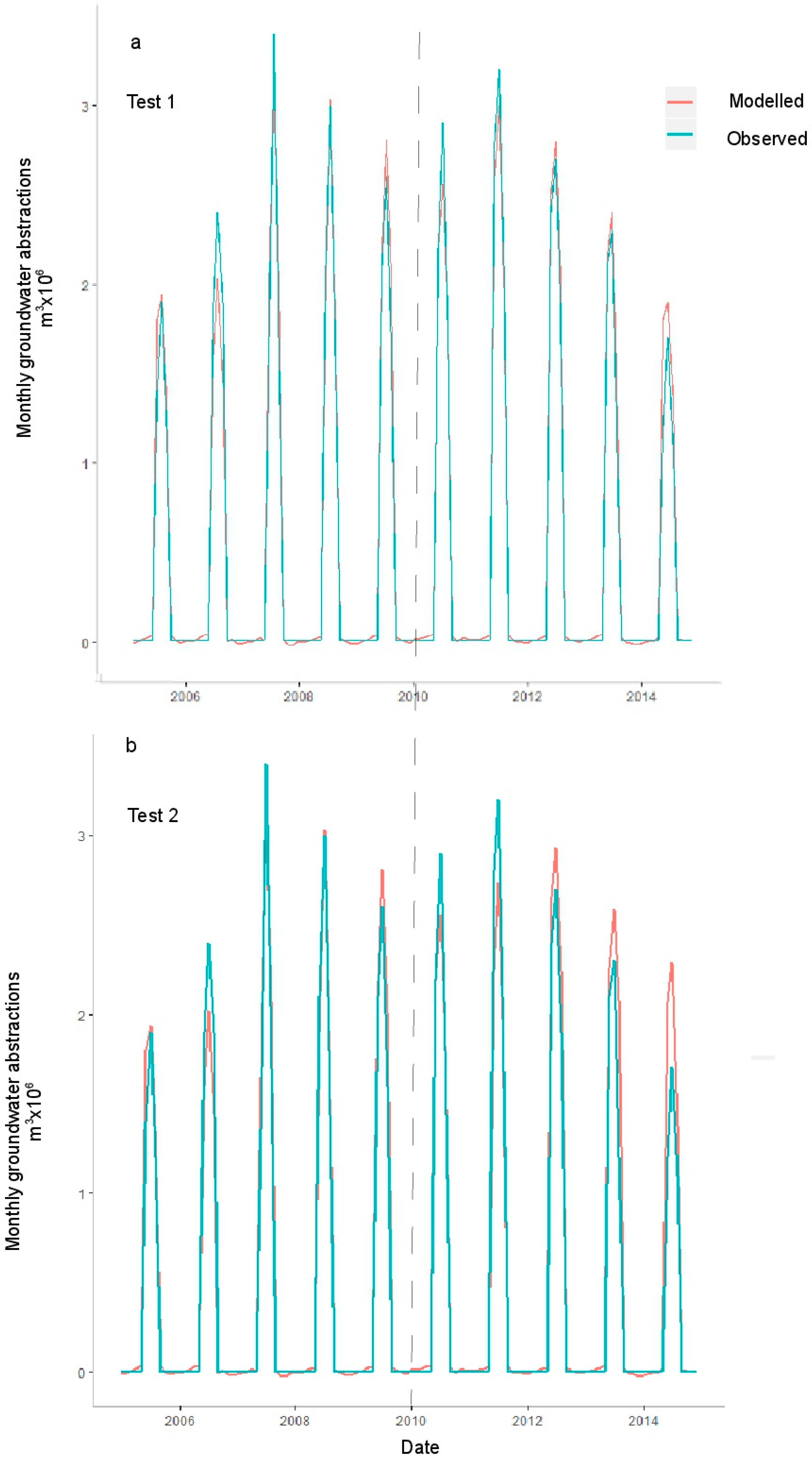
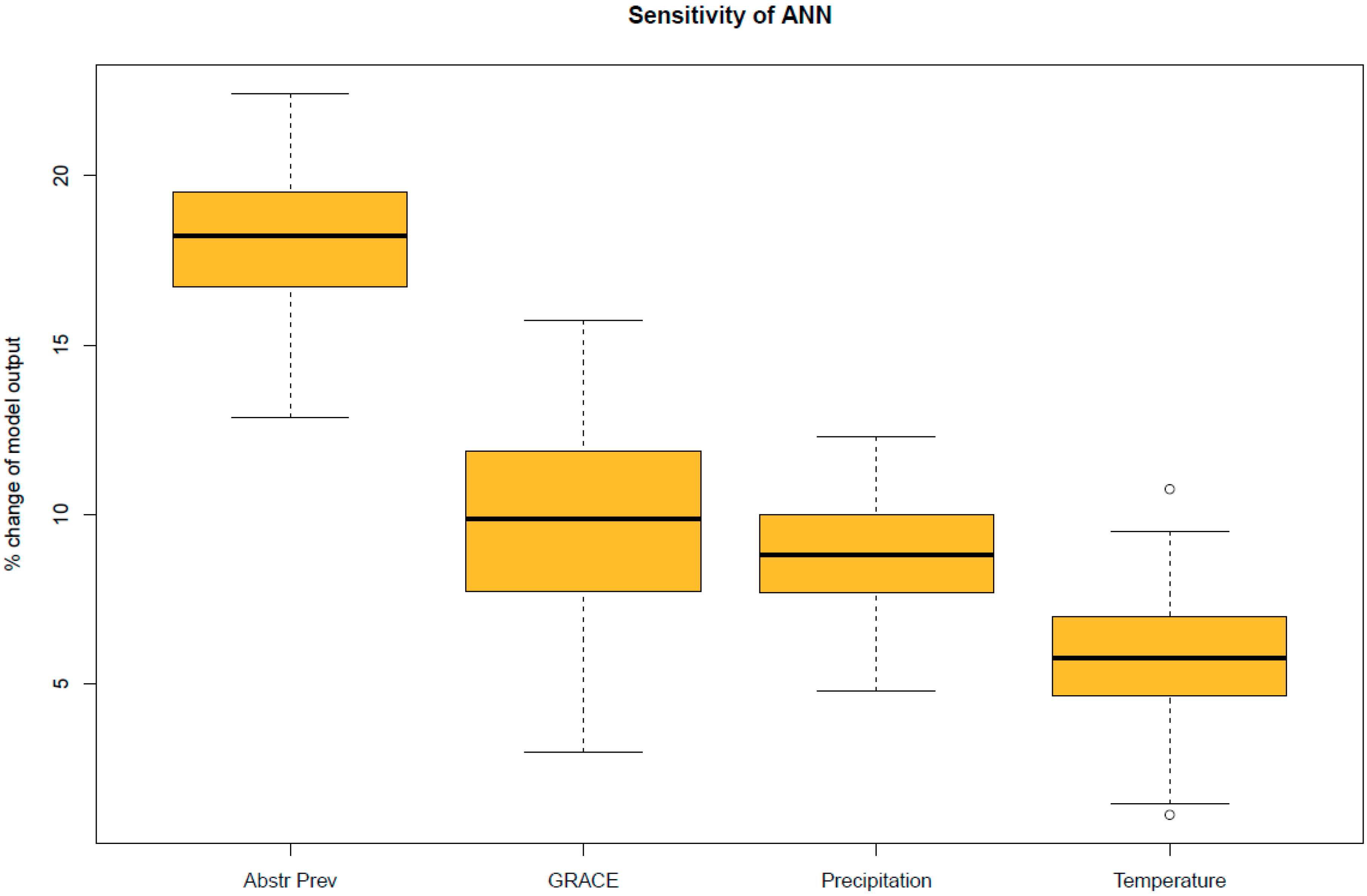
3. Results and Discussion

Results of the cross-correlation analysis for predictor variables with the target variable, i.e., monthly groundwater abstractions, are summarized on

Table 2. Cross correlation and auto-correlation analysis results.

Parameter	Cross-Correlation Function	Time Lag (Months)
Monthly precipitation	−0.3	0
Mean monthly temperature	0.72	0
GRACE Total Water Storage anomalies—ΔTWS	−0.33	0
Monthly groundwater abstractions	0.89 *	12

* Corresponds to auto-correlation function of monthly groundwater abstractions.

.

Cross-correlation analysis showed a high positive correlation of 0.72 for the temperature with groundwater abstractions at lag 0 (current time step). Monthly precipitation and monthly GRACE ΔTWS demonstrated negative correlation with monthly groundwater abstractions of −0.3 and −0.33, respectively, at lag 0. No statistically significant correlations were detected at other time lags. Additionally, as groundwater abstraction time series demonstrates strong autocorrelation, the autocorrelation function (ACF) at various lags was examined, and a strong autocorrelation of 0.89 was evidenced at lag 12 (abstractions at the same month of the previous year), which is an expected outcome considering the seasonality of groundwater abstractions [17]. Results in Table 2 indicate that all examined variables may well serve as predictors in the ANN model, and therefore input variables were determined to be monthly precipitation, mean monthly temperature, monthly abstractions at lag 12, and GRACE monthly ΔTWS. It should be noted herein that correlation coefficient is an indicator that expresses the linear relationship between two variables and may not reveal the possible non-linear relationships. ANNs however have proved to be capable to approximate the causal relationship of any non-linear dynamic system [10].

Secondly the architecture of ANN was determined. To keep the model as simple as possible, one hidden layer was involved, which is satisfactory for most applications. A critical issue which impacts model performance and convergence speed, is the number of hidden neurons, which is usually estimated by trial and error. An empirical rule calls for a number of hidden neurons to range between half and twice the number of predictors [10]. In our work, we examined various combinations of input variables and hidden layer architecture as presented in

Table 3. Performance metrics of ensemble ANNs in the testing phase.

Input Variables	Architecture *	R*	NSE
Abstractions (Lag 12)	3 3:1	0.35	0.77
Mean monthly temperature GRACE monthly ΔΤWS	3:4:1	0.31	0.79
Abstractions (Lag 12)	3 3:1	0.41	0.72
GRACE monthly ΔTWS Monthly precipitation	3:4:1	0.38	0.78
Abstractions (Lag 12)	3:3:1	0.44	0.65
Mean monthly temperature Monthly precipitation	3:4:1	0.41	0.69
GRACE monthly ΔTWS	3:3:1	0.91	0.43
Mean monthly temperature Monthly precipitation	3:4:1	0.88	0.45
Abstractions (Lag 12)	4:3:1	0.29	0.82
Mean monthly temperature	4:4:1	0.23	0.95
Monthly precipitation	4:5:1	0.31	0.80
GRACE monthly ΔTWS	4:6:1	0.35	0.78

* First number corresponds to input neurons, second to hidden layer neurons and third to output neurons.

. The best results in terms of performance metrics were acquired for four input and four hidden layer neurons, thus the ANN architecture in this work is 4:4:1. The architecture and synapse weights of the developed ANN are shown on Figure 3.

Performance metrics for Test 1 and Test 2 refer both to the testing period of the ANN. Figure 4 shows plots of the results of the application of the developed ANN. Both models were found to be very good based on their performance metrics (NSE > 0.75 and R* < 0.50) [36]. Test 1 ensemble performance metrics at the testing phase were: R* = 0.23 and NSE = 0.95. Test 2 ensemble performed with R* = 0.31 and NSE = 0.86 at the testing phase. Both models capture the trend of monthly groundwater abstraction time series and they both estimated with satisfactory accuracy the abstracted quantities. Considering the minimum data requirements of Test 2, however, it is considered as a reasonable approach for the estimation of abstracted groundwater quantities. In both models, the worst prediction was observed for 2014 when an extraordinary rainy and cool summer was observed, with precipitation exceeding that of the months of the training period.

Relative importance of input variables was estimated using the weight connection method described above, and the results showed that monthly groundwater abstractions at lag 12 is by far the most important predictor (Figure 5). This is not a surprising finding since monthly groundwater abstractions demonstrate great seasonality and therefore seasonal lags are expected to play an important role in the modeling process. The next almost equally important factors are GRACE ΔTWS and monthly precipitation, whereas temperature seems to be the least important variable in the modeling process, despite its high correlation with the target variable. This finding can be potentially explained considering the high seasonality of both groundwater abstractions and temperature. In our case, seasonality of the target variable is represented by the auto-correlative component (at lag 12) and therefore the predictive ability of temperature is considerably downgraded.

To test the sensitivity of our model to uncertainties in the input parameters we examined the inherent properties of input variables. Mean monthly temperature and monthly precipitation are directly measured and the uncertainty to those variables is expected to be low. Groundwater abstractions are indirectly estimated and therefore the uncertainty related to this variable is expected to be higher and might influence model results. The highest uncertainty however is related to the GRACE ΔTWS data. GRACE data possess inherent uncertainties because of their coarse nature that differs significantly from that of the hydrological data sets [11,13]. Nevertheless, recent techniques have provided finer scaled gridded data (~100 km) applying gridded gain factors [20]. Those gridded data were used in the present work. Scaled GRACE data, applying gridded gain factors are reported to possess errors ranging from 36 mm water-equivalent height at low latitudes, to <15 mm at polar areas [20]. According to that work [20], the expected error of data in the latitude of Greece amounts ~20 mm of water, which accounts for approximately 15% of the GRACE monthly ΔTWS data range for the study area. We therefore performed sensitivity analysis by changing each time one input variable randomly within the range of ±15%, and quantifying change in the model output.

Results of sensitivity analysis, presented in Figure 6, indicate that the developed model is mostly sensitive to changes in groundwater abstraction at lag 12, where a 15% change results in an average of 18% change in model output. Sensitivity to GRACE data is found to be around 10%, thus indicating that the ANN model is moderately sensitive to the variable with the highest uncertainty. Model sensitivity to precipitation is determined to approximately 9%, whereas temperature is the parameter where the model is least sensitive to. A change of 15% in mean monthly temperature results in approximately 6% change in model results.

Our results indicated the usefulness of GRACE data, which has also been found in previous works [10]. Additionally, our findings indicate that GRACE ΔTWS can be downscaled and used along with in situ meteorological data to estimate water quantities abstracted from an aquifer body. Previous works have shown the usefulness of GRACE observations for predicting groundwater level changes [1,10] or for estimation of water storage changes is surface reservoirs [38]. Only recent studies showed that groundwater storage changes even at local scales can be estimated with GRACE data [1]. Although groundwater storage changes are different in their nature from groundwater abstractions, as changes in storage of groundwater incorporate the natural and human induced changes, whereas groundwater abstractions are only related to human activities, our work supports our argument that GRACE may well contribute to determination of groundwater extraction quantities even for local groundwater bodies. It was also shown that even in the case of complex groundwater–surface water interactions, which is the case of Neon Sidirochorion aquifer, such a methodology performs sufficiently well, as GRACE data, due to their coarse nature, describe changes in TWS of the broader area and serve as an indicator of the regional pattern of water changes which is probably reflected at the local scales. The relative importance of GRACE ΔTWS shows thus to what extent regional TWS changes are reflected at the local scale. Such a methodology is especially useful when a monitoring network has failed to provide required abstracted quantities and may help water managers to identify aquifers being at risk of quantitative stress. They may then enforce measures to ensure balance between abstractions and recharge, thus contributing to the restoration of the groundwater system.

4. Conclusions

In the present work, an ANN model has been developed to estimate monthly groundwater abstracted quantities from an aquifer body, using in situ meteorological data and GRACE remotely sensed observations as input variables. Results showed that gridded GRACE ΔTWS can be downscaled and used for estimating abstracted quantities of groundwater. As the whole process uses readily available meteorological data and remotely sensed GRACE data, it is a reasonable and low-cost alternative when the monitoring network fails to provide such information. After development, training, and testing of an ANN which requires expert knowledge and computational skills, it is thereafter a readily available tool for use by water managers. The methodology is especially useful for areas like Greece, where groundwater represents approximately 42% of the total water demand, and other analogous cases where groundwater constitutes a major source of water.

References

1. Miro, M.E.; Famiglietti, J.S. Downscaling GRACE remote sensing datasets to high-resolution groundwater storage change maps of California’s Central Valley. Remote Sens. 2018, 10. [Google Scholar] [CrossRef]
2. Taylor, C.; Alley, W. Ground-Water-Level Monitoring and the Importance of Long-Term Water-Level Data; USGS Circular 1217; US Geological Survey: Reston, VA, USA, 2001.
3. Brunner, P.; Hendricks Franssen, H.-J.; Kgotlhang, L.; Bauer-Gottwein, P.; Kinzelbach, W. How can remote sensing contribute in groundwater modeling? Hydrogeol. J. 2007, 15, 5–18. [Google Scholar] [CrossRef]
4. Wada, Y.; Van Beek, L.P.H.; Van Kempen, C.M.; Reckman, J.T.M.; Vasak, S.; Bierkens, M.P. Global depletion of groundwater resources. Geophys. Res. Lett. 2010, 37, 1–5. [Google Scholar] [CrossRef]
5. Döll, P. Vulnerability to the impact of climate change on renewable groundwater resources: A global-scale assessment. Environ. Res. Lett. 2009, 4, 1–12. [Google Scholar] [CrossRef]
6. Giorgi, F. Climate change hot-spots. Geophys. Res. Lett. 2006, 33, L08707. [Google Scholar] [CrossRef]
7. Giorgi, F.; Lionello, P. Climate change projections for the Mediterranean region. Glob. Planet. Chang. 2008, 63, 90–104. [Google Scholar] [CrossRef]
8. Neteler, M. Estimating daily land surface temperatures in mountainous environments by reconstructed MODIS LST data. Remote Sens. 2010, 2, 333–351. [Google Scholar] [CrossRef]
9. Alsdorf, D.E.; Rodriguez, E.; Lettenmaier, D.P. Measuring surface water from space. Rev. Geophys. 2007, 45, 1–24. [Google Scholar] [CrossRef]
10. Sun, A.Y. Predicting groundwater level changes using GRACE data. Water Resour. Res. 2013, 49, 5900–5912. [Google Scholar] [CrossRef] [Green Version]
11. Lakshmi, V. Beyond GRACE: Using Satellite Data for Groundwater Investigations. Groundwater 2016, 54, 615–618. [Google Scholar] [CrossRef] [PubMed] [Green Version]
12. Richey, A.S.; Thomas, B.F.; Lo, M.-H.; Reager, J.T.; Famiglietti, J.S.; Voss, K.; Swenson, S.; Rodell, M. Quantifying renewable groundwater stress with GRACE. Water Resour. Res. 2015, 51, 5217–5238. [Google Scholar] [CrossRef] [PubMed] [Green Version]
13. Gemitzi, A.; Lakshmi, V. Evaluating Renewable Groundwater Stress with GRACE Data in Greece. Groundwater 2018, 56, 501–514. [Google Scholar] [CrossRef] [PubMed]
14. Long, D.; Scanlon, B.R.; Longuevergne, L.; Sun, A.Y.; Fernando, D.N.; Save, H. GRACE satellite monitoring of large depletion in water storage in response to the 2011 drought in Texas. Geophys. Res. Lett. 2013, 40. [Google Scholar] [CrossRef] [Green Version]
15. Gemitzi, A.; Petalas, C.; Pisinaras, V.; Tsihrintzis, V.A. Spatial prediction of nitrate pollution in groundwaters using neural networks and GIS: An application to South Rhodope aquifer (Thrace, Greece). Hydrol. Process. 2009, 23, 372–383. [Google Scholar] [CrossRef]
16. Gemitzi, A.; Stefanopoulos, K.; Schmidt, M.; Richnow, H.H. Seawater intrusion into groundwater aquifer through a coastal lake—Complex interaction characterised by water isotopes 2H and 18O. Isotopes Environ. Health Stud. 2014, 50, 74–87. [Google Scholar] [CrossRef] [PubMed]
17. Gemitzi, A.; Stefanopoulos, K. Evaluation of the effects of climate and man intervention on ground waters and their dependent ecosystems using time series analysis. J. Hydrol. 2011, 403, 130–140. [Google Scholar] [CrossRef]
18. Gemitzi, A. Evaluating the anthropogenic impacts on groundwaters; a methodology based on the determination of natural background levels and threshold values. Environ. Earth Sci. 2012, 67, 2223–2237. [Google Scholar] [CrossRef]
19. Swenson, S.C. GRACE monthly land water mass grids Netcdf Release 5.0; Ver. 5.0. Physical Oceanography Distributed Active Archive Center, CA, USA. 2012. Available online: https://podaac.jpl.nasa.gov/dataset/TELLUS_LAND_NC_RL05 (accessed on 8 August 2017).
20. Landerer, F.W.; Swenson, S.C. Accuracy of scaled GRACE terrestrial water storage estimates. Water Resour. Res. 2012, 48, 1–11. [Google Scholar] [CrossRef]
21. Wahr, J.; Molenaar, M.; Bryan, F. Time-variability of the Earth’s gravity field: Hydrological and oceanic effects and their possible detection using GRACE. J. Geophys. Res. 1998, 103, 30205–30230. [Google Scholar] [CrossRef]
22. Tapley, B.D.; Bettadpur, S.; Ries, J.C.; Thompson, P.F.; Watkins, M.M. GRACE Measurements of Mass Variability in the Earth System. Science 2004, 305, 503–505. [Google Scholar] [CrossRef] [PubMed] [Green Version]
23. Faour, K. Winter Crop Budgets, Southern Zone 2001; NSW Agriculture: Leeton Shire, Australia, 2001. [Google Scholar]
24. Coulibaly, P.; Anctil, F.; Aravena, R.; Bobée, B. Artificial neural network modeling of water table depth fluctuations. Water Resour. Res. 2001, 37, 885–896. [Google Scholar] [CrossRef] [Green Version]
25. Chu, H.-J.; Chang, L.-C. Optimal control algorithm and neural network for dynamic groundwater management. Hydrol. Process. 2009, 23, 2765–2773. [Google Scholar] [CrossRef]
26. Coppola, E.A.; Szidarovszky, F.; Davis, D.; Spayd, S.; Poulton, M.M.; Roman, E. Multiobjective analysis of a public wellfield using artificial neural networks. Ground Water 2007, 45, 53–61. [Google Scholar] [CrossRef] [PubMed]
27. Huang, Z.; Pan, Y.; Gong, H.; Yeh, P.J.; Li, X.; Zhou, D.; Zhao, W. Subregional-scale groundwater depletion detected by GRACE for both shallow and deep aquifers in North China Plain. Geophys. Res. Lett. 2015, 42, 1791–1799. [Google Scholar] [CrossRef] [Green Version]
28. Scanlon, B.R.; Longuevergne, L.; Long, D. Ground referencing GRACE satellite estimates of groundwater storage changes in the California Central Valley, USA. Water Resour. Res. 2012, 48, 1–9. [Google Scholar] [CrossRef]
29. Tachi, S.E.; Ouerdachi, L.; Remaoun, M.; Derdous, O.; Boutaghane, H. Forecasting suspended sediment load using regularized neural network: Case study of the Isser River (Algeria). J. Water Land Dev. 2016, 29, 75–81. [Google Scholar] [CrossRef] [Green Version]
30. Zhou, Z.-H. Ensemble Methods: Foundations and Algorithms; Taylor & Francis Group, LLC: Abingdon, UK, 2012; ISBN 9781439830055. [Google Scholar]
31. Dietterich, T.G. Ensemble Methods in Machine Learning. In Multiple Classifier Systems; Kittler, J., Roli, F., Eds.; Springer: Heidelberg, Germany, 2000; pp. 1–15. ISBN 978-3-540-67704-8. [Google Scholar]
32. Fritsch, S.; Guenther, F.; Suling, M.; Mueller, S.M. Package ‘Neuralnet’; The Comprehensive R Archive Network: Hoboken, NJ, USA, 2016. [Google Scholar]
33. Legates, D.R.; McCabe, G.J., Jr. Evaluating the Use of “Goodness of Fit” Measures in Hydrologic and Hydroclimatic Model Validation. Water Resour. Res. 2005, 35, 233–241. [Google Scholar] [CrossRef]
34. Groenendijk, P.; Heinen, M.; Klammler, G.; Fank, J.; Kupfersberger, H.; Pisinaras, V.; Gemitzi, A.; Peña-Haro, S.; García-Prats, A.; Pulido-Velazquez, M.; et al. Performance assessment of nitrate leaching models for highly vulnerable soils used in low-input farming based on lysimeter data. Sci. Total Environ. 2014, 499, 463–480. [Google Scholar] [CrossRef] [PubMed]
35. Nash, J.E.; Sutcliffe, J.V. River Flow Forecasting Through Conceptual Models Part I—A Discussion of Principles*. J. Hydrol. 1970, 10, 282–290. [Google Scholar] [CrossRef]
36. Moriasi, D.N.; Arnold, J.G.; Van Liew, M.W.; Bingner, R.L.; Harmel, R.D.; Veith, T.L. Model Evaluation Guidelines for Systematic Quantification of Accuracy in Watershed Simulations. Trans. ASABE 2007, 50, 885–900. [Google Scholar] [CrossRef]
37. Olden, J.D.; Joy, M.K.; Death, R.G. An accurate comparison of methods for quantifying variable importance in artificial neural networks using simulated data. Ecol. Model. 2004, 178, 389–397. [Google Scholar] [CrossRef]
38. Wang, X.; De Linage, C.; Famiglietti, J.; Zender, C.S. Gravity Recovery and Climate Experiment (GRACE) detection of water storage changes in the Three Gorges Reservoir of China and comparison with in-situ measurements. Water Resour. Res. 2011, 47, 1–13. [Google Scholar] [CrossRef]
Figure 1. Location map of the study aquifer. Neon Sidirochorion aquifer indicated by blue line.
Geosciences 08 00419 g001
Figure 2. Time series plots of monthly precipitation, mean monthly temperature, monthly groundwater abstractions and GRACE monthly ΔTWS from 2005–2014.
Geosciences 08 00419 g002
Figure 3. ANN architecture and synapse weights. Black lines correspond to input-hidden layer weights. Blue lines denote hidden-output layer weights. Precip corresponds to monthly precipitation, Temp stands for mean monthly temperature, GRACE corresponds to monthly GRACE ΔTWS, and AbstrPrev denotes monthly groundwater abstractions at lag 12.
Geosciences 08 00419 g003
Figure 4. Observed and modelled time series of monthly groundwater abstractions for two performed tests. Vertical dotted line separates training period (2005–2009) from testing period (2010–2014).
Geosciences 08 00419 g004
Figure 5. Relative importance of input variables in the developed ANN.
Geosciences 08 00419 g005
Figure 6. Sensitivity of the ANN model to 15% uncertainty of input parameters. Abstr Prev: Monthly groundwater abstractions at lag 12, GRACE: GRACE monthly ΔTWS changes, Precipitation: Monthly precipitation, Temperature: Mean monthly temperature.
Geosciences 08 00419 g006