Article

Automatic Coastline Extraction Using Edge Detection and Optimization Procedures

by
Vasilis Paravolidakis
1,
Lemonia Ragia
2,*,
Konstantia Moirogiorgou
1 and
Michalis E. Zervakis
1
1
School of Electronic and Computer Engineering, Technical University of Crete, Kounoupidiana, 73100 Chania, Greece
2
School of Environmental Engineering, Technical University of Crete, Kounoupidiana, 73100 Chania, Greece
*
Author to whom correspondence should be addressed.
Geosciences 2018, 8(11), 407; https://doi.org/10.3390/geosciences8110407
Submission received: 19 August 2018 / Revised: 21 October 2018 / Accepted: 4 November 2018 / Published: 7 November 2018

Abstract

:
Coastal areas are quite fragile landscapes as they are among the most vulnerable to climate change and natural hazards. Coastline mapping and change detection are essential for safe navigation, resource management, environmental protection, and sustainable coastal development and planning. In this paper, we proposed a new methodology for the automatic extraction of coastline, using aerial images. This method is based on edge detection and active contours (snake method). Initially the noise of the image is reduced which is followed by an image segmentation. The output images are further processed to remove all small spatial objects and to concentrate on the spatial objects of interests. Then, the morphological operators are applied. We used aerial images taken from an aircraft and high-resolution satellite images from a coastal area in Crete, Greece, and we compared the results with geodetic measurements, to validate the methodology.

1. Introduction

Coastal areas have emerged to be the most important and dynamic regions, worldwide. They are unique areas on earth because they are the connection between sea and land. They encompass a rich ecosystem with a high diversity of species. Due to climate change, they are environmentally the most sensitive. Global warming effects like sea-level rise, coastal erosion, warmer water temperature, changes in the intensity of waves have been widely prevalent, in recent years [1]. Coastline is a line that forms the boundary between the land and the sea, or a lake [2].
Global warming causes sea-level rise and consequently it will affect most of the world’s coastlines through inundation and increased erosion [3]. The coastal areas are among the most vulnerable to climate change and natural hazards, making them fragile landscapes. Flooding, erosion, sea-level rise, as well as extreme weather events, are some of the most common natural hazards we encounter. An additional negative factor is human interventions. For example, in the Greek coastline about 30 percent is affected by erosion caused from human intervention [4].
This paper describes the automatic extraction of the coastline using edge detection and optimization procedures. We present a new approach of a pre-existing estimation algorithm for coastline extraction, based on the Canny edge detection [5] and the locally adaptive thresholding methods, introduced by Liu and Jezek [6]. Their background work has been enhanced and altered in order to produce smoother and more reliable results. We have also added another feature to their approach, the active contour-fitting, in order to optimize the results and extract the final model of the coastline.

2. Previous Work

2.1. Satellite Images

In recent years, satellite imagery has been used in semi-automatic or automated coastline extraction and mapping from high-resolution images. Different approaches use Synthetic Aperture Radar (SAR) data. Erteza [7] made one of the first attempts at presenting an automated approach that comprises three main algorithms for coastline extraction. Dellepiane et al. [8] introduced an innovative algorithm able to semi-automatically extract the coastline, using an InSAR (Interferometric Synthetic Aperture Radar). Modava and Akbarizadeh [9] developed a combination of two algorithms, the image classification and the active contours, to extract the coastline from the SAR images. The COSMO-Beach system uses multitemporal SAR techniques for a semi-automatic shoreline extraction and coastal morphology [10].
Moreover, multispectral images have been extensively used for coastline extraction. First, Braud and Feng [11] and subsequently Frazier and Page [12], evaluated the threshold-level slicing and multispectral (especially Band 5 of Landsat TM) image classification techniques for the detection of coastline. Zhang et al. [13] used multispectral remote sensing images to extract the coastline in an aquaculture coast.
Di et al. [14] performed a semi-automatic approach for coastline extraction from IKONOS image, based on the mean shift segmentation algorithm, water body identification, and a local refinement. Another paper proposes an approach in two steps, based on morphological tools, to extract the coastline, according to their context, from the Quickbird multispectral (MS) images [15]. Landsat-8 images have also been used for coastline extraction [16]. Sekovski et al. [17] employed a WorldView-2 MS image to depict coastline by integrating different supervised and unsupervised image classification techniques.

2.2. Aerial Images

Aerial images taken by aircraft were the only source of environmental management, until the SAR and LIDAR technologies were developed. Thus, aerial images were the most commonly used data source in coastline mapping and they also give us access to historical coastline estimations. Distinguishing land and water in grayscale or black and white aerial images, especially where the waters are blurry and muddy, requires extensive terrestrial efforts. Moreover, due to the fact that aerial images were not digital, the extraction of information is difficult and mistake-prone. Here, we outline some of the previous work.
Automatic extraction of the shoreline features from aerial images has been investigated using neural networks and image processing techniques. Ryan et al. [18] used an image segmentation method to approach the coastline extraction problem and tested their method on several small portions (256 × 256) of scanned US Geological Survey (USGS) aerial photographs. They applied a neural network method on a texture measure of the images, to separate the land and water regions. The use of texture influenced the accuracy and the need for training the neural nets limited this approach to a large volume of full-scene image data.
Chalabi et al. [19] developed a coastline extraction method for satellite and aerial images, based on segmentation techniques (Pixel-based segmentation or grey-level thresholding). This method segments an image, based on a digital number (DN) threshold [20]. An unsupervised classification was then applied to classify similar pixel values in a group and give them a tag. In order to convert the raster data into vector data, two attributes were used, one for the classes with a value of 1 and all other classes were set to 0. The shoreline was then exported to a GIS environment and vectorized using the ArcInfo software (Esri, Redlands, CA, USA).
Liu and Jezek [6] introduced a comprehensive approach for an automated extraction of the coastline, from satellite imagery, but it could also apply to aerial image data. It consists of a sequence of image processing algorithms, in order to reduce noise and enhance the major edges.
Yousef and Iftekharuddin [21] applied a fusion of aerial images and LIDAR digital elevation models data, using genetic algorithms, for the purpose of coastline extraction. The LIDAR data and the aerial images are fused, by maximizing their mutual information through a genetic algorithm [22], assuming both images have the same spatial coverage, the same spatial resolution, and are georeferenced to a common grid. Additionally, support vector machines classify the fused data and segment it into land and water pixels. This approach can work without reference to a tidal datum, as described on LIDAR imagery and can extract the shoreline. This approach yields accurate results, when compared to ground data, but bears the cost of the LIDAR image data. Willersley [23] proposes two methods, one based on sub-pixel resolution and the other on minimum noise fraction for extracting the coastline from satellite images.
Finally, in recent years video systems have been used for coastline extraction. Valentini et al. [24] used a new tool for automatic shoreline detection and data analysis using automatic segmented Timex images, derived from a video monitoring system. The great number of video images allows for Machine Learning techniques. HoonHout et al. [25] delineated the Smooth Support Vector Machine for region classification of coastal areas. Coastal change monitoring is an important topic for environmental issues. Lisi et al. [26] presented a method for beach morphodynamic classification, using Timex images. Plant et al. [27] presented an algorithm for bathymetry estimation from video images for quantitative near-shore monitoring and prediction.

3. The Proposed Approach

This paper presents an extension of our work that appeared in Reference [28]. We use more data and extend our methodology to incorporate satellite images. In addition, we test the robustness of the methodology using in-situ geodetic measurements. The algorithms have been modified to improve the performance of the pixel-enhancement phase. For the automatic coastline extraction, in this paper we have introduced a new version of the method presented by Liu and Jezek [6], relying on edge detection and optimization procedures.
Our methodology follows two main stages. The first stage provides an estimation of the coastline, based on region segmentation techniques, using a local thresholding method. The second stage optimizes the results of the first stage and models the coastline, based on active contours. Particularly as a first step, we reduce the noise and enhance the edges of the image. As a second step, we split the image into blocks, for the purpose of finding a threshold related to local characteristics. As a third step, we apply morphological operations and edge detection to obtain the coastline. As a fourth step, we apply an active contour method, in order to get better results.
The proposed method uses input image data that were provided by the Hellenic Military of Geographical Service (HMGS) [29] and multispectral satellite images, provided by a private company.

3.1. Data Pre-Processing

Two primary procedures are applied at the pre-processing step so that it is possible to perform the image segmentation. The first procedure filters the image noise to reduce the noisy edges in the subsequent image segmentation. The second procedure enhances the edges along the coastline, while suppressing other unimportant edges inside the land or the sea area.

3.1.1. Noise Reduction and edge enhancement

Aerial images can provide a good spatial coverage of the coast but they are also inevitably distorted by noise. The deformation of the image by unexpected factors, sunlight, shadows or clouds, can lead us to wrong results. For these reasons, we apply the anisotropic diffusion algorithm, as presented by Perona and Malik [30]. This algorithm aims to enhance strong edges, along the coastline, or to suppress weak edges inside the sea or the land area. Figure 1 shows the effect of the filtering step using the Gaussian, Median, and Mean filters. Applying Gaussian filter is the most efficient filtering method for our images. It removes the noise, while keeping the image smooth. On the contrary, although the median and mean filters remove the noise, they blur the image edges, especially in the coastline area. Visually it is not very clear, but in practice, blurring the edges will lead us to wrong estimations. The anisotropic diffusion also reduces the weak edges, while the strong edges along the coastline are enhanced, as shown in Figure 2.

3.1.2. K-means Clustering

The first phase includes a clustering of the image, using K-means. K-means clustering treats each object of the image as having a location in space. It finds partitions, such that objects within each cluster are as close to each other as possible, and as far from objects in other clusters, as possible. K-means clustering requires that you specify the number of clusters to be partitioned and a distance metric to quantify how close two objects are to each other. In our work we chose to have three clusters and to use the Euclidean distance metric. More specifically, Cluster 0 corresponds to the sea pixels, while Cluster 1 and Cluster 2 correspond to the land pixels. We ended up choosing three clusters, by taking into consideration experimental results on a variety of image data. Less or more clusters will eventually lead to the production of non-homogeneous regions.

3.2. Image Region Segmentation

The second step of our methodology is the region segmentation. We aim to split the image into two regions, land and sea. The coastline is composed of the pixels that belong to the borders of the two regions. We use local thresholds in order to separate the land objects from the water background. A global threshold would lead to false estimations, as a result of the image intensity heterogeneity. Therefore, we developed a region segmentation algorithm using local thresholds, based on local characteristics.

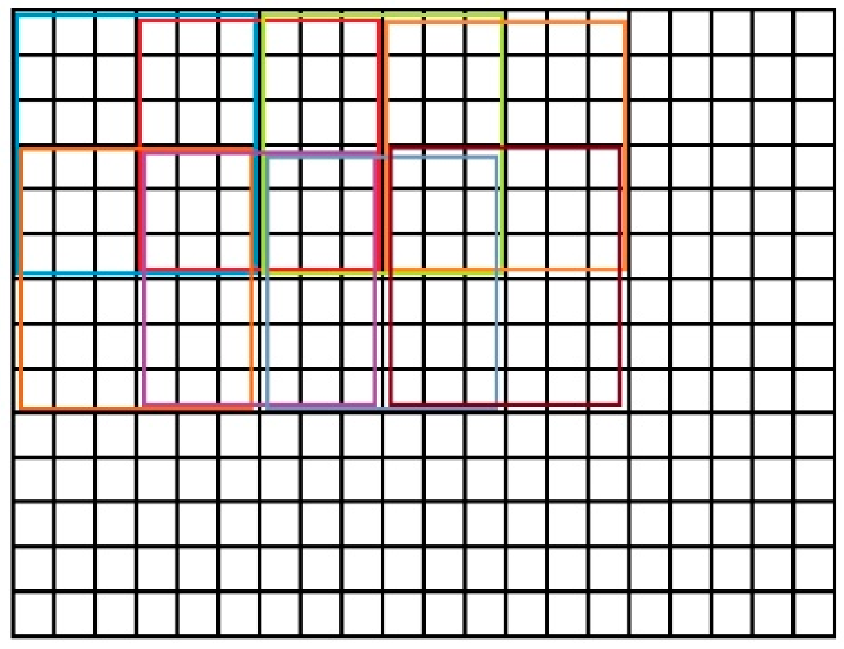
3.2.1. Block Division and Local Thresholding

We divide the image into small blocks and find a threshold for each of them. The purpose of this subdivision is that homogeneous blocks that involve only sea or land pixels need no further processing. After many empirical tests, we found out that for images with a size of 4000 × 4000 pixels the best block size would be 200 to 300 pixels.
In Figure 3 a sample of the process through which the overlapping blocks are applied to an image, is shown. Each rectangle refers to a pixel of the image while a colored rectangle refers to a block.

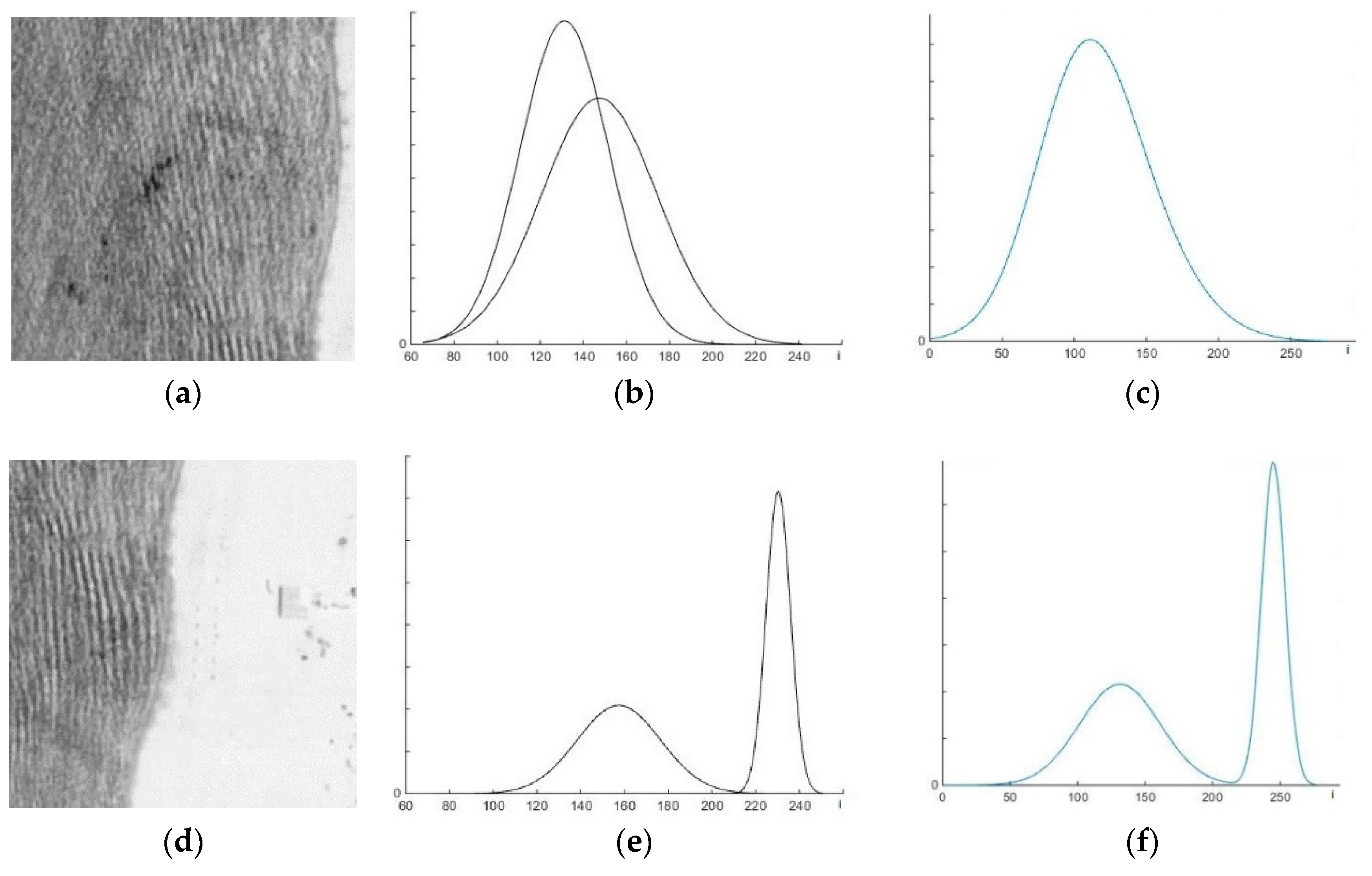
3.2.2. Local Thresholds

At this point we try to distinguish the pixels that refer to water, from the rest of the land. Initially, we are looking for the blocks that have a value of zero, according to K-means algorithm. If a block has more than 90% zero values, then no further processing is required. For the remaining blocks, there are two Gaussian distributions, one for the water and the other for the land.
For the remaining blocks, we examine the bimodality. More specifically, we assume that there are two Gaussian distributions of the intensity values, one for the description of the water and the other for the land. Their combination generates a Gaussian mixture model, describing the observed intensity values of the image. If a block contains mostly water or land area pixels, the mixture of the distribution will only reflect one peak (unimodal). On the other hand, if a block is part of the coastline area, the mixture of distributions will consist of one valley and two peaks (bimodal).
The probability density of a Gaussian distribution F(x) is given by Equation (2).
F ( x ) = 1 2 π σ e ( x μ ) 2 2 σ 2
where x is the gray level, μ is the mean of the distribution, and σ stands for standard deviation. The probability destiny function p(z) of a mixture of two Gaussian distributions F1(x) and F2(x) is given by Equation (3).
p ( z ) = p 1 F 1 + p 2 F 2
and
p 1 + p 2 = 1
Combining the previous Equations (2) and (3), results in the following Equation (4):
p ( z ) = p 1 2 π σ 1 e ( x μ 1 ) 2 2 σ 1 2 + 1 p 1 2 π σ 2 e ( x μ 2 ) 2 2 σ 2 2
where μ1 and μ2 is the mean of the two distribution, σ1 and σ2 are the standard deviations, and p1 is the coefficient of the mixture, which shows the ratio between the total number of sea area pixels and total size of blocks in pixels. Then we used a simple Expectation Maximization (EM) of the Gaussian Mixture Model (GMM) algorithm [31], in order to compute the above five parameters of the mixture of the Gaussian distributions. In the first step of this algorithm, the Expectation obtains expected values for the missing data, using an initial parameter estimate based on the K-means. It then follows the Maximization step, where ‘i’ is the maximum likelihood estimation of the parameters that is obtained, using the estimated data. This procedure will repeat until the estimate converges.
After having the Gaussian distributions parameters computed, we are able to test the bimodality by using three criteria. First, we need to compute the valley-to-peak ratio of the total histogram of the block according to Equation (5):
δ = M i n { p ( i ) } μ 1 < i < μ 2 M i n { p ( μ 1 ) , p ( μ 2 ) }
where, p is the Gaussian curve fitted in the previous steps and μ1 < i < μ2. In our applications, we want a valley-to-peak ratio of δ < 0.9. Second, the means of the two-component distribution must differ by more than 10 gray levels.
Lastly, the Ashman’s D parameter is required to be greater than two for a clean separation of the two distributions [32]. In Equation 6 it is shown that Ashman’s parameter is a combination of the means and the standard deviations.
D = ( 2 1 2 ) | μ 1 μ 2 | σ 1 2 + σ 2 2
A block that would pass all three criteria is shown in Figure 4d, which, as it can be seen, consists of a coastline area, while a block that would fail at the first criterion is also shown in Figure 4a, an image that mostly consists of sea.
For every block that passes the bimodality tests, a threshold T is calculated by using the Otsu method [33]. This method automatically performs the clustering-based image thresholding of a grayscale image, by maximizing the weighted within-class variance. The algorithm follows the assumption that the block contains two classes of pixels (land, sea), through a bimodal histogram (already established from the previous step) and then calculates the optimum threshold that classifies the two classes so that their combined spread is minimal. The weighted within-class variance is expressed by:
σ w 2 ( t ) = q 1 ( t ) σ 1 2 ( t ) + q 2 ( t ) σ 2 2 ( t )
where weights qi are the probabilities of the two classes being separated by a threshold t, and σi2 denote the variances of these classes. Using an iterative process for every t in 1 ≤ T ≤ 256, we can compute the threshold that minimizes the between-class variance. We apply the threshold to each block of the image and create a binary one, following the procedure below:
b ( x , y ) = { 0 , for I ( x , y ) T 1 , for I ( x , y ) > T }
where T is the threshold of the block and I(x, y) is the intensity value of the image pixel at points x, y. For every block that fails to pass the bimodality test, a binary image is created with zero values, at every point.

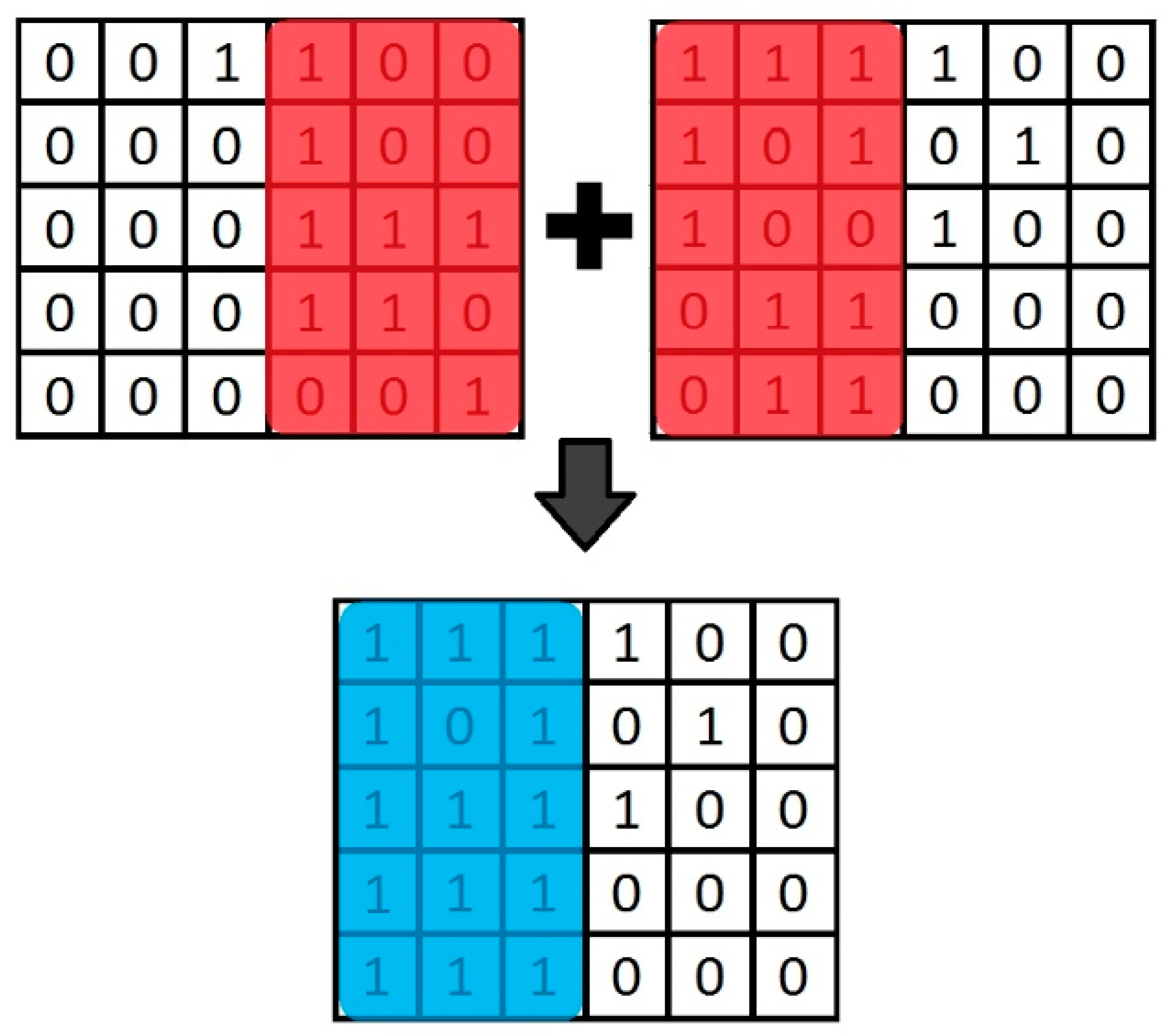
3.3. Data Post-Processing

At the last step of our approach, we concatenate the blocks in order to recreate the image in a binary class form. The final value of each pixel is calculated by following the logic ‘OR’ condition between the overlapping areas, which assigns the value 1 for the final pixel if and only if one of the overlapping blocks is 1, at this point. To explain why we use this procedure, we remind that blocks with over 90% of pixels in the sea area do not pass the bimodality test. However, in extreme cases, a small part of the coastline may be involved in such a block. It is expected that a neighboring block will identify the coastline because it will contain both parts of the water and the land area. The use of the proposed conjunction condition aims to protect such edge pixels, across the coastline that appear only at a portion of the overlapping blocks.
In Figure 5 we can see an example of the concatenation procedure between two sample blocks and the block produced after post-processing. This procedure continues until the input image is fully recreated in the binary form.
The binary form of the image is followed by the removal of false-positive waves, ships, or other objects on the sea surface that can lead us to a false edge recognition in this area. To eliminate these effects, we apply the morphological operations of erosion and dilation. An erosion procedure followed by a dilation one removes small objects, while preserving the original abstract shape of the image. The structure element H that we would use for the morphological operations would be specified in a way that stray foreground structures that are larger than H, would have to be preserved. Furthermore, we apply a closing operation, which is a dilation followed by an erosion. This operator fills black holes smaller than the structure element H, but also keeps the original shape of the image. Additionally, the binary form of the image is followed by a region grouping, in order to code the water pixel as 0’s and the land pixels as 1’s. This will produce two large continuous land and water objects.
Finally, we use a simple edge detection operator to detect edges in the image. Notice that at this stage of processing, the binary image involves a white area that belongs to land and a black area that belongs to sea, so that the boundary line refers to the coastline. We used the Canny edge detection method, which operates in three steps: (a) Find the intensity gradient of the image, (b) apply the non-maximum suppression, where pixels that are not considered to be part of an edge are removed, and (c) hysteresis is applied to eliminate gaps. The result constitutes the first estimation of the coastline.

3.4. Coastline Modeling

The estimated coastline needs further improvement, due to spatial objects that are close to coastline, such as waves or constructions. In order to deal with these problems, we adopt an open active contour method, which is based on snakes and extends the classical active contour model introduced by Kass et al. [34], with the condition of free boundary conditions. Active contours have been proposed for image segmentation for different data sets [35]. We initialize this curve using the already extracted coastline, obtained from the first approach. More specifically, a snake is an energy-minimizing spline that consists of an initial closed contour C0 near to a contour in the image and searches for deformations of C0 which move it towards the actual image contour. To obtain these deformations we need to minimize the energy functions, formed by the two energy terms, regarding the intensity distribution of the image around the edge and reflect the internal and external regions of the edge itself. This function can be expressed as follows:
E s n a k e = 0 1 ( α | C ( s ) | 2 + β | C ( s ) | 2 λ | ( I ( C ( t ) ) | ) d t
where C(s) = (x(s), y(s)), s ∈ [0, 1] is the initial curve in the original Image I, parameters α and β impose the elasticity and rigidity of the curve, parameter λ determines the level of the gradient regions that the curve will attract to, and ∇I is the gradient of the image intensity.
In most images of our case study, the land is separated from the sea by a vertical or horizontal curve positioned from the top to bottom or from left to right of the image, respectively, so that the endpoints of coastline are parts of the image margins. Thus, our approach needs to handle the case of an open curve. There are three types of open active contour characterized by their boundary conditions, namely, (1) fixed boundaries, where the curve has two end points that cannot change through the curve evolution; (2) no boundaries, where there are no endpoint and the final curve may be deflected; and (3) free boundaries, where the two endpoints will belong to two curves (boundary curves). We adopted Shemesh and Ben-Shahar’s method [36] to develop a process using active contours, with free boundary conditions. By default, the boundary curves will lie on the top and the bottom of the image, based on our image data, but they can manually be changed in order to fit every possible circumstance. To be more specific, first, we need to initialize the curve C(s). This will happen automatically by extracting the coastline, based on region segmentation. Then, assuming the energy function of the curve C(s) is limited to first order derivatives, it can be generalized as:
E s n a k e ( C ( s ) ) = 0 1 H ( x , y , x , y ) d s
where H refers to both, the internal and the external term and can result in the Euler-Lagrange equations shown below:
H x d d s H x = 0 ;   H y d d s H y = 0
Now going back to Equation (11), for simplicity we assume that β = 0 and applying Equation (11) onto it, will produce the following Euler equations:
2 α x + θ θ x ( λ | I ( C ( s ) ) | ) = 0
2 α y + θ θ y ( λ | I ( C ( s ) ) | ) = 0
This can provide us a complete equation for calculating the curve C(s), over time:
C ( s , t ) = 2 α C ( s , t ) + g ( s , t )
where C(s,t) represents the curve at iteration ‘t’, and g(s,t) = −λ|∇I(C(s))|. We also know that the two endpoints of the curve C(s,t) are restricted to lie on the two boundary curves one of which is at the bottom of the image and the other one at the top of the image. Let B0: [0,1] be the first boundary curve and q be the parameter value where C(s) crosses the boundary curve. The expressions that shows us the restrictions for the first endpoint (q0) are:
( H x , H y ) s = 0 * ( X 0 , Y 0 ) = ( H x , H y ) s = 0 * B 0 | q = 0
where Hx = Hx (x, y, x0, y0), Hy = Hy (x, y, x0, y0), s = 0 is the first point of the curve C(s) and X0, and Y0 are the coordinates of the curve B0 at point q0. Respectively, for the second endpoint:
( H x , H y ) s = 1 * ( X 1 , Y 1 ) = ( H x , H y ) s = 1 * B 1 | q = 1
Now, by applying Equations (16) and (17) to H functions, we get the following restrictions that are necessary to be verified, in order to keep the endpoints at the boundary curves.
2 α ( x , y ) | s = 0 * ( X 0 , Y 0 ) = 0
2 α ( x , y ) | s = 1 * ( X 1 , Y 1 ) = 0
In our method, we use one boundary curve on the top and one on the bottom of the image. We followed this procedure because we wanted an automated method of coastline extraction and the image dataset provides us this facility. We can now estimate, iteratively, the next possible position of the curve (coastline), by minimizing the energy of the snake, for 150 iterations. The number of iterations is based on experiments for our image dataset.

4. Results

The experimental analysis of the aforementioned approach has shown that we had carried out an accurate coastline estimation. All the data was referred to the Greek Geodetic Reference System GGRS87. We performed our method to many data sets, in order to be persuaded of the accuracy and robustness of the algorithm. We used the existing images data from the coastal area of the region Georgioupoli, located at North West Crete, Greece. Two data sets were analyzed and presented explicitly in this study. One set came from the photogrammetric method and the other from remote sensing. The aerial image data were provided by the Hellenic Military Geographical Service. We also used Satellite Multispectral images. To be convinced that the methodology works well, we compared the results for the coastline to the coastline obtained by the “ground truth”, using in-situ geodetic measurements.

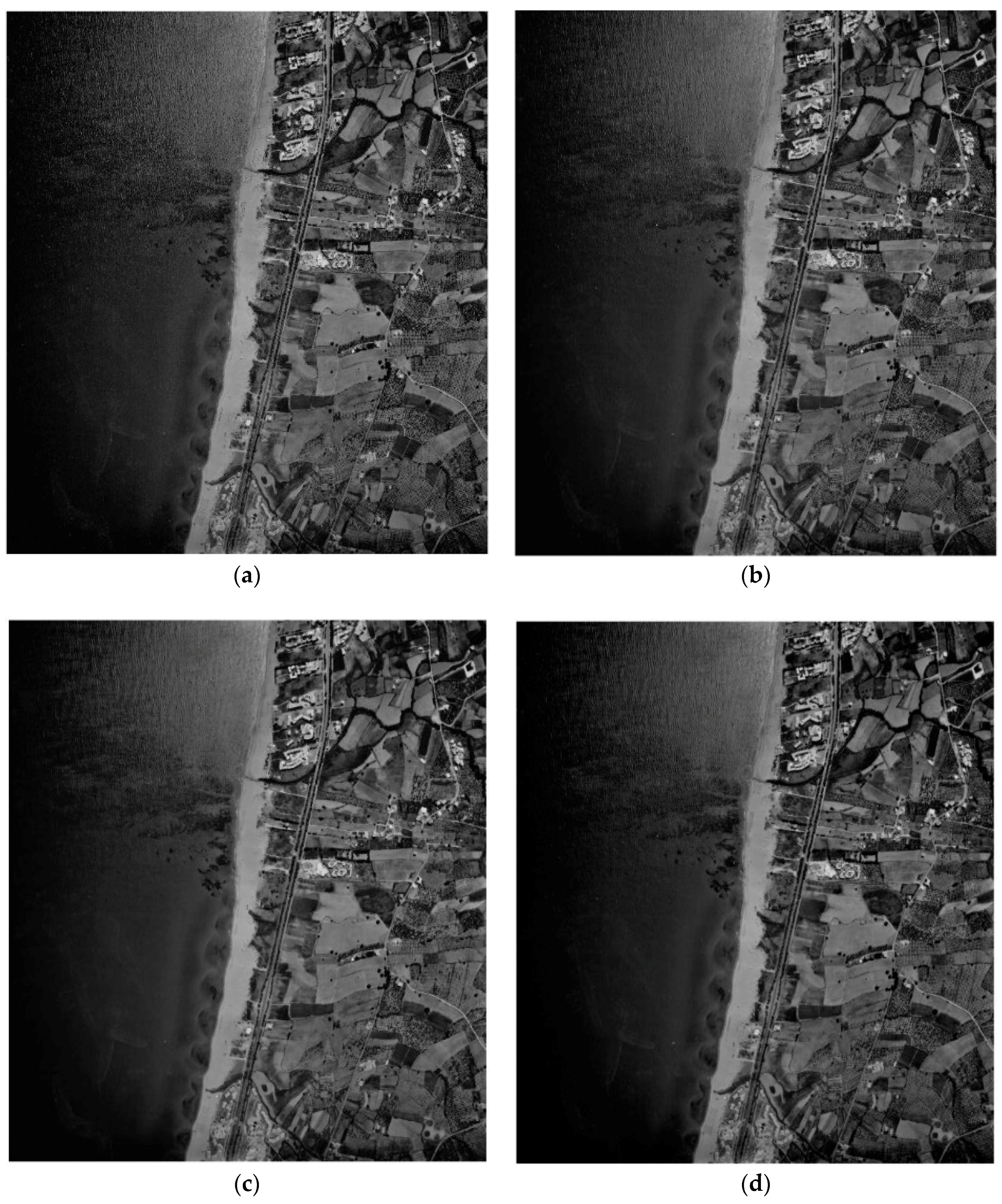
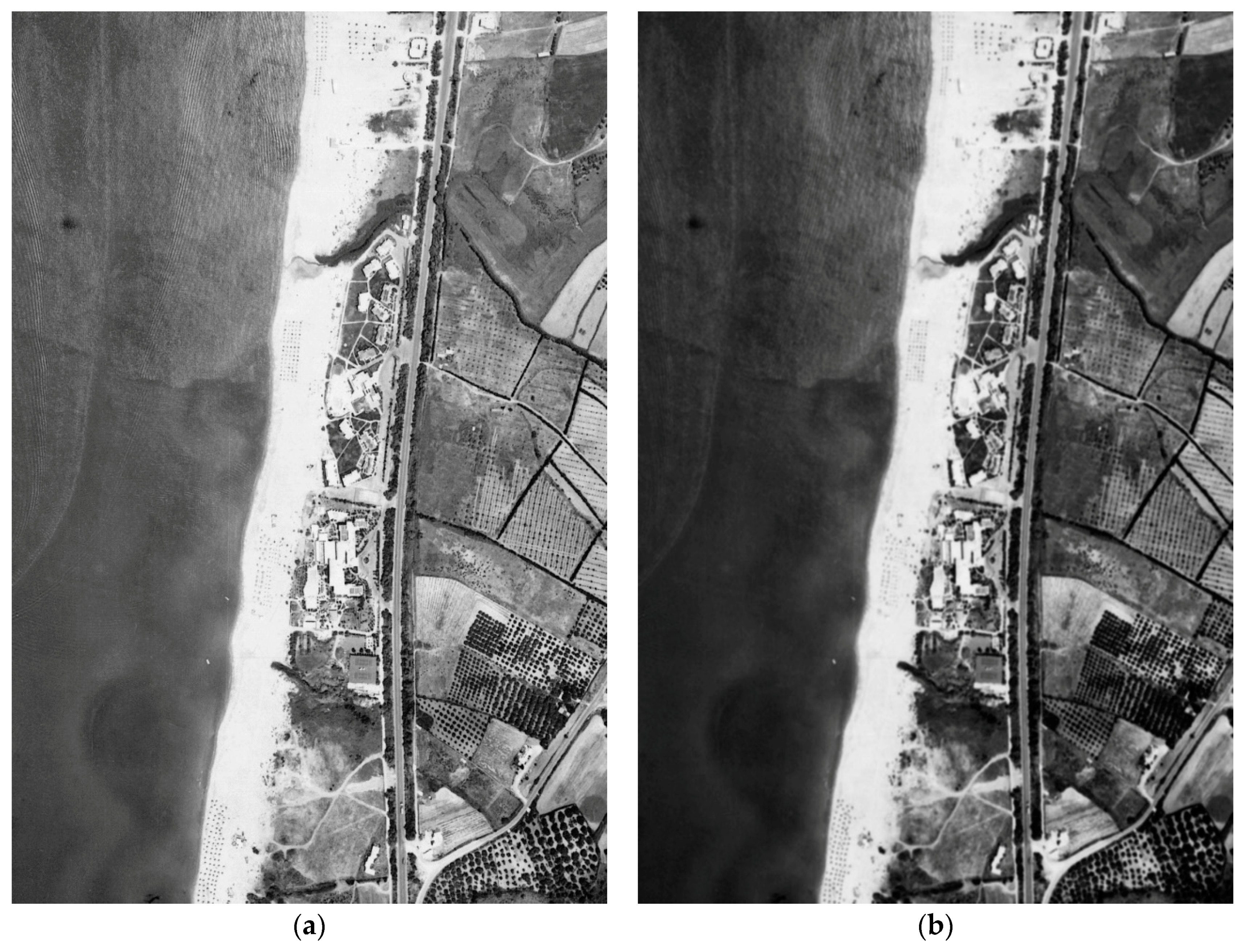
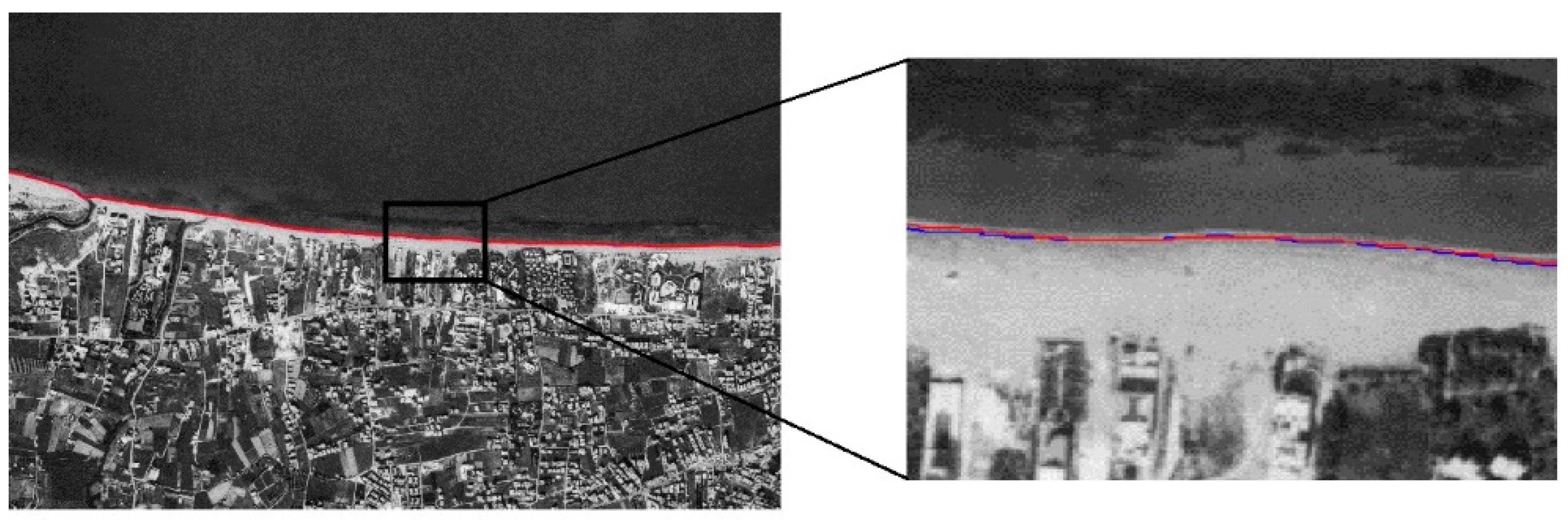
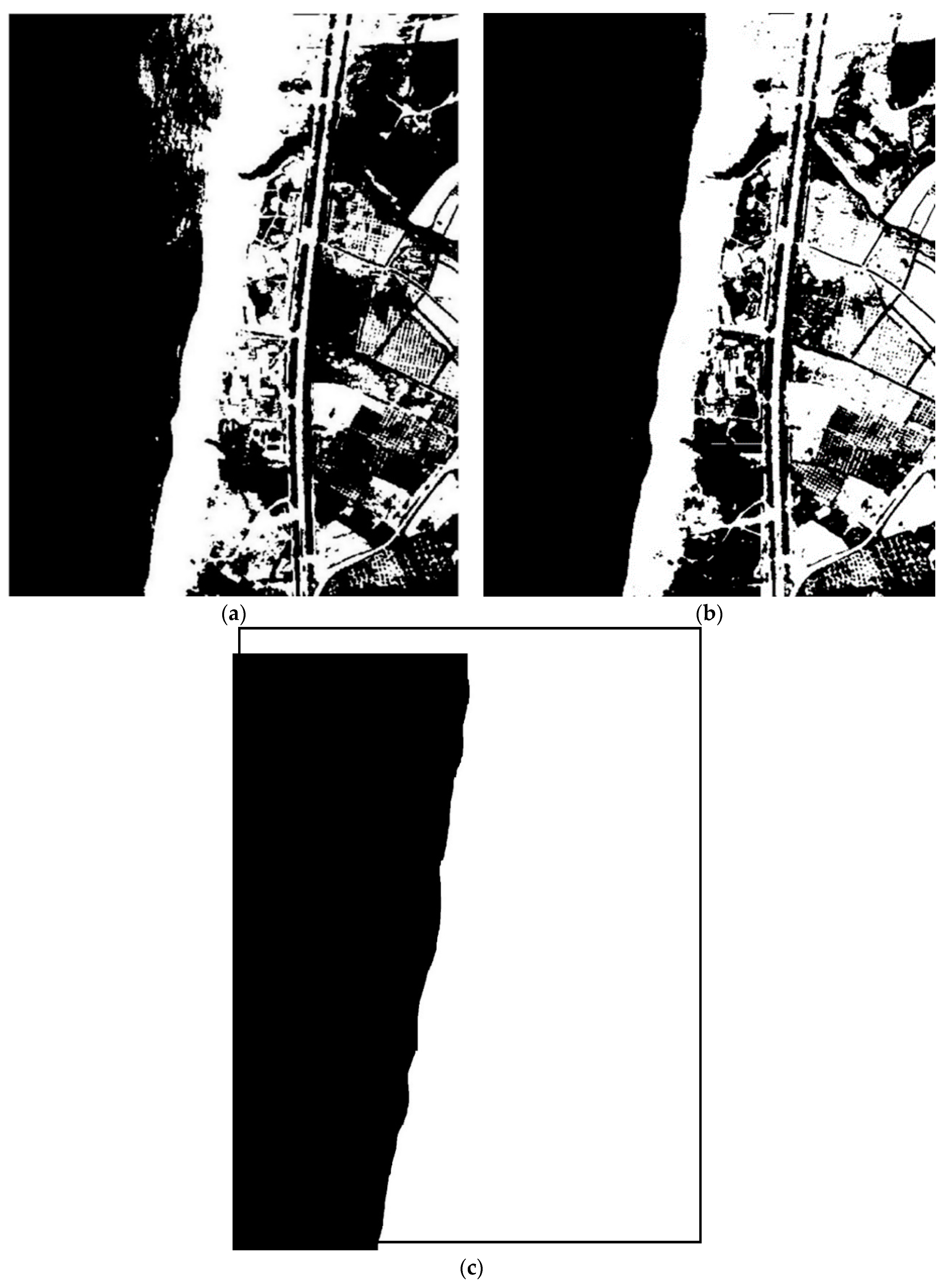
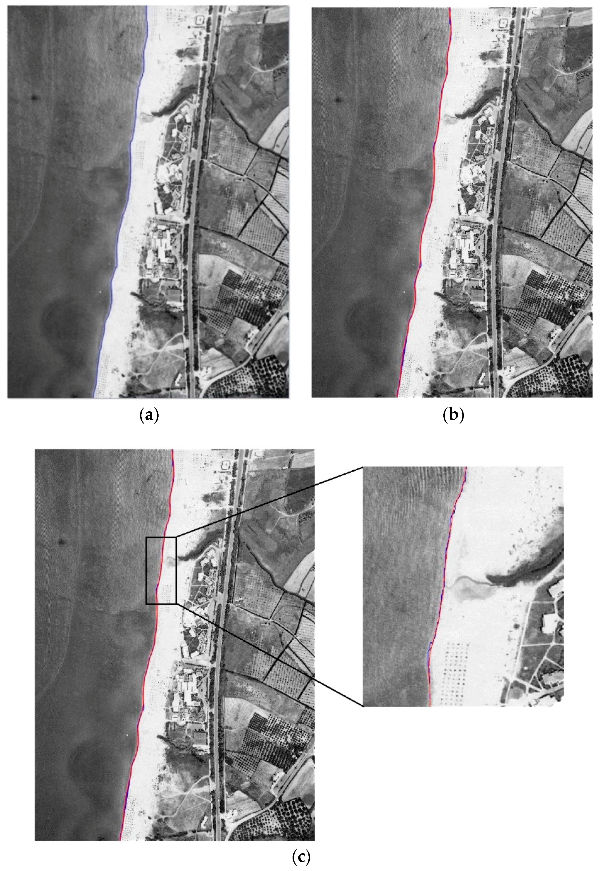
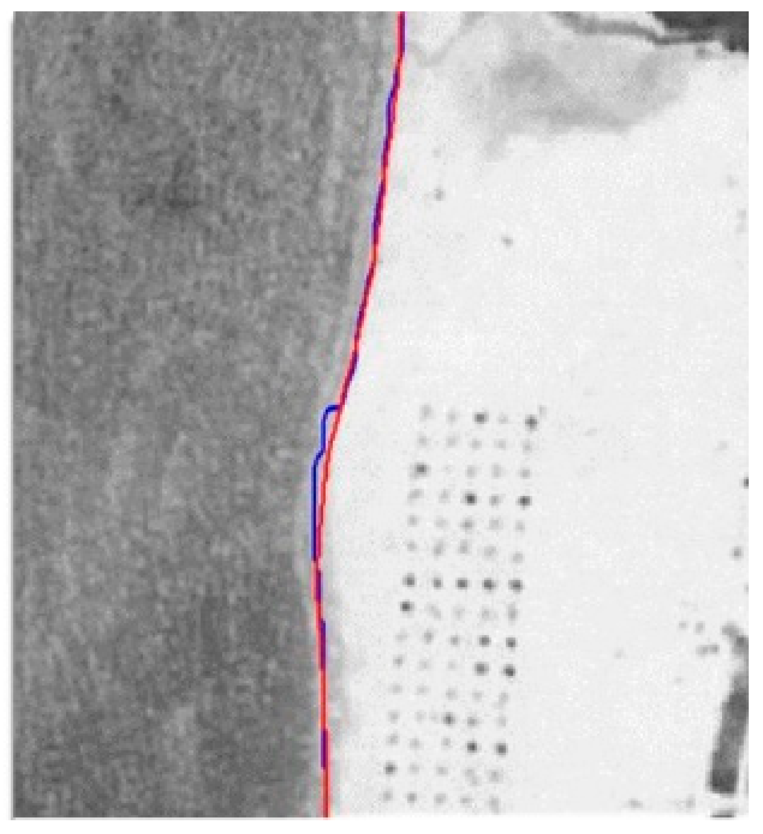
4.1. Coastline Extraction Using Aerial Images

The aerial images used in this example were acquired by the Hellenic Military Geographical Service (HMGS), during the period of 1990 to 2005, taken by aircraft and were free for use from the Greek Cadastre. The first set of images were approximately 5200 × 5400 pixels and were taken from a height of 1550 m. The images had a spatial resolution of 15 cm on the earth. The second set of images were 1920 × 1080 and had a spatial resolution of 20 cm. By applying our method to the aerial images, we had successfully extracted a complete, accurate coastline, across the region of Georgioupoli, Crete, Greece. Figure 6 illustrates the processing sequence applied to the first aerial image Figure 6a. The Gaussian filter and then the anisotropic diffusion operator was applied to the image, which was the pre-processing step. At this phase the image noise was considerably reduced, intensity variations and weak edges inside the land or the ocean were effectively suppressed, while the coastline edges were enhanced, as shown in Figure 6b.
At the next step, we applied the k-means algorithm to cluster the image into two regions, land and sea Figure 7a. Subsequently, the entire image was divided into overlapping image regions, each with 400 × 400 pixels. Fifteen percent of the image regions that had a high variance were selected for analytically determining the optimal local thresholds. The five bimodal Gaussian parameters were computed and then a threshold was computed for every region that met the three criteria of bimodality. The concatenated image is shown in Figure 7b. Afterwards, at the post-segmentation processing stage, region grouping was applied with the aim of creating a homogeneous area, where the land pixels value was 1 while the sea pixels value was 0. Additionally, the morphological operators removed the noisy image objects (Figure 7c). Finally, we extracted the coastline by using a canny edge detection procedure and proceeded to the next step.
At this point, we applied the coastline modeling. An automatic initialization of the active contours took place, using the outcome of the previous step. In Figure 8, the final estimated coastline with a close-up, for a better identification of the changes, is shown. The blue line in Figure 8a refers to the estimated coastline extracted from the first approach, while the red line in Figure 8b refers to the optimized coastline obtained from the second approach. Comparing the two results, the added benefits of the curve-fitting, resulting in smoother estimates that are less affected by other physical formations close to the coastline, can be seen (Figure 8c and Figure 9).
Figure 10 presents the results from the methodology, using the second set of aerial images. In this case, we needed to manually change the boundary curves of the active contour. Now they lay on the left to right instead of the default position of the top to bottom of the image. Once again, it was easily understood that the second approach improved the initial estimation of the region segmentation, offering visually valid results. We needed to convert the image from RGB to Grayscale, in order to be processed from our algorithm. This image had the same ’behavior’ as a digitized aerial image and we expected good estimations. In Figure 11, it was shown that our method led to good coastline estimations. In this case, again, the blue line refers to the estimated coastline extracted from the first approach, while red line refers to the optimized coastline obtained from the second approach.

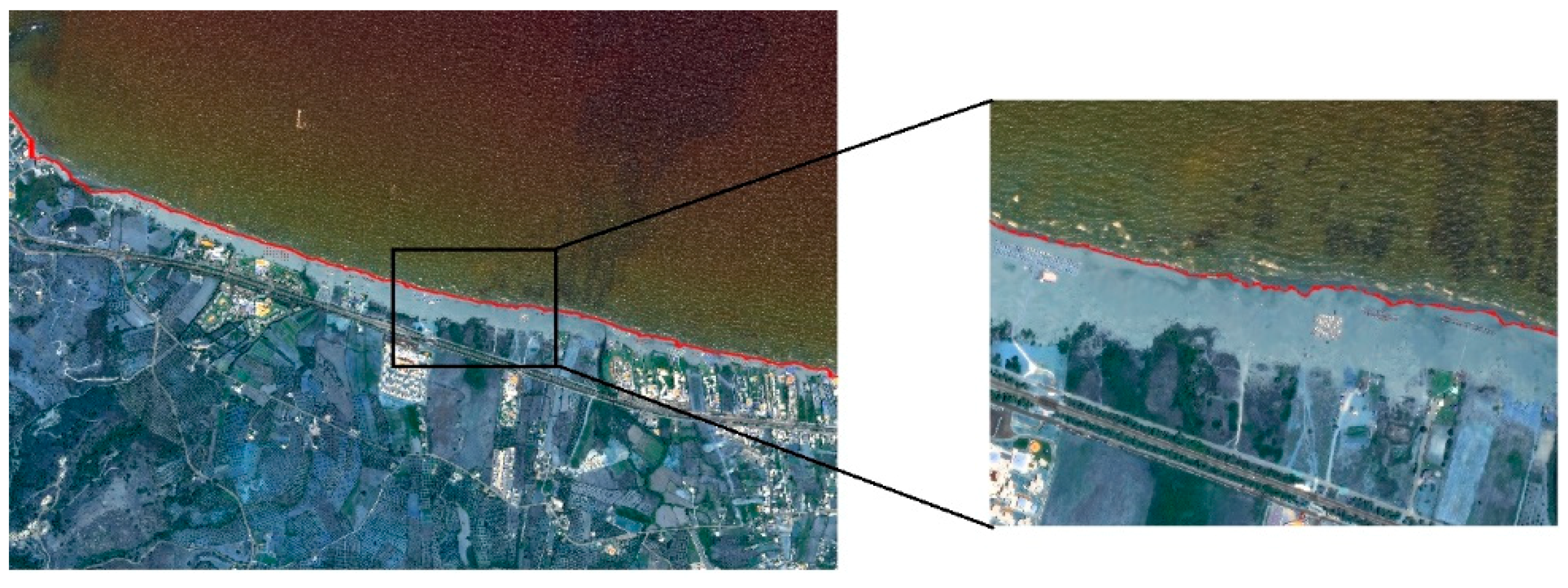
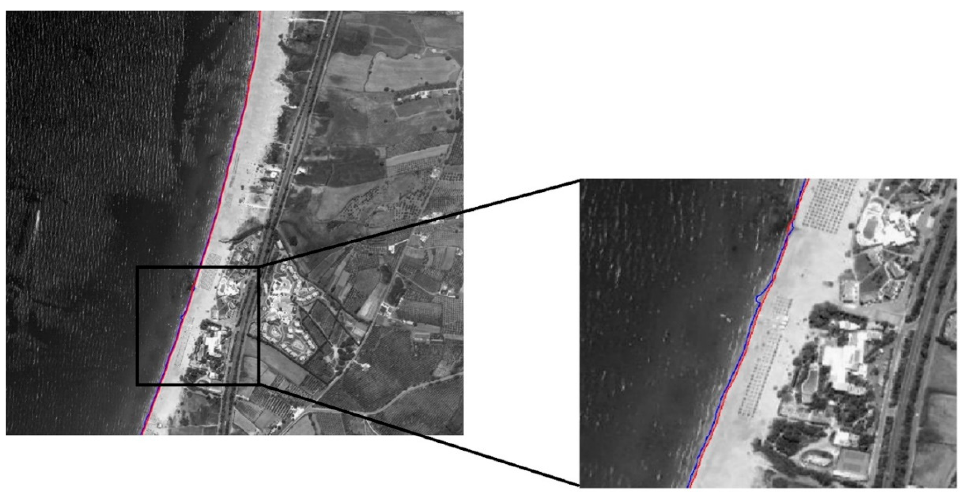
4.2. Coastline Extraction Using Satellite Images

The most common data used these days for coastline extraction are Satellite Images. We examined how our method applied to high-resolution multispectral images. We used the WorldView-2 satellite images, taken on July 2016, with 30 cm spatial resolution and 18,206 pixel width and 17,007 pixel height. This type of image, is capable of providing a good estimate. As can be seen in Figure 12, our algorithm provided a reliable estimation.
Our aim was to provide a coastline estimation algorithm, and thus, no optimization attempts were made. Our approach took approximately 40 s, for the first stage (approach 1), and up to 1.65 min, for the optimization step. This performance speed was the average computation speed for the various image sizes. The most time-consuming component was the computation of the next curve, which consumed, approximately, 69% of the computational time. The computational speed could be largely improved, by optimizing the algorithm of the coastline modeling and effectively reducing the resolution of the images, in order to reduce the computational cost.
We have historical aerial images of Greece (taken in airplanes), from 1929 until 2000, with a spatial resolution of 10 cm per pixel. These images have already been used for many years for the monitoring and assessment of coastal erosion. From 2000 onwards, we only have satellite images with different spatial resolution, starting from 30 cm per pixel. This in practice meant that using our methodology with historical aerial images before the year 2000 and satellite images after 2000, we can draw conclusions on the changes of the coastline and consequently of the erosion of the area. As a result, it is possible to map the coastline erosion over many years, combining data coming from aerial photographs and from satellite images.
Finally, to perform an assessment of the accuracy of the proposed method a set of recognizable ground control points were surveyed, using Global Navigation Satellite System (GNSS). Since the satellite images provide geo-referenced information, as a result, the estimated coastline could be compared to the “ground truth” measurements (Figure 13). We used 55 Ground Control Points (GCPs) to compare our results, using a GPS receiver of an accuracy of 50 cm. The instrument was a topographic differential GPS Topcon Hiper pro. The GPS survey was performed at the same year as the acquisition of the satellite image within two months. The area is microtidal with the mean tidal being 60 cm [37]. There was, definitely, a difference between the two survey methods, the photogrammetry, and the geodesy. Using the Root Mean Square Error, we found an error of 0.85 m, which is an accepted accuracy for such a fuzzy object like coastline and it seems to be better than that obtained from other approaches [10].

5. Conclusions

The present approach provides an automated coastline extraction methodology, using aerial images, through image processing techniques aimed at region segmentation and edge detection. Following the elimination of possible noise distortion in the input data and the enhancement of the edges of interest, through an anisotropic diffusion algorithm, we applied a region segmentation, in order to split the image into two groups of regions—land and sea. The processes of thresholding, edge detection, and active contour-fitting improved the accuracy of the extracted coastline.
Additionally, we developed a framework, through which a user can load the images of interest, perform a coastline extraction, view the results, and, finally, calculate the useful parameters, using the distance or area metrics, by taking advantage of the connection of the results with the cadastral data.
As for future work, we intend to improve the accuracy of the coastline estimation. This can be implemented by using the geo-referenced images and can provide a pixel-to-real-distance conversion, i.e., pixels/cm conversion scheme. Furthermore, this conversion might provide a robust basis for post-processing and computation of real-world measures, such as coastline length, coast surface, and erosion levels.

Author Contributions

Conceptualization, L.R. and K.M.; Investigation, V.P.; Methodology, M.E.Z.; Software, V.P.; Supervision, K.M. and M.E.Z.; Validation, L.R. and K.M.; Writing—original draft, V.P.; Writing—review & editing, L.R.

Funding

This research received minor external funding from project sMart fArming with dRoneS—MARS.

Acknowledgments

This research has been co-financed by the European Union and Greek national funds through the Operational Program Competitiveness, Entrepreneurship and Innovation, under the call RESEARCH—CREATE—INNOVATE (project code: T1EDK-04759, project name: sMart fArming with dRoneS—MARS).

Conflicts of Interest

The authors declare no conflict of interest.

References

  1. Church, J.A.; White, N.J. Sea-Level Rise from the Late 19th to the Early 21st Century. Surv. Geophys. 2011, 32, 585–602. [Google Scholar] [CrossRef] [Green Version]
  2. Coast. Available online: https://en.wikipedia.org/wiki/Coast (accessed on 25 September 2018).
  3. Effect of Climate Change on Coastline Evolution. Available online: http://www.coastalwiki.org/wiki/Effect_of_climate_change_on_coastline_evolution (accessed on 25 September 2018).
  4. Aμμος κατά διάβρωσης. Available online: http://www.haniotika-nea.gr/116521-ammos-kata-diabrwsis/ (accessed on 10 May 2018).
  5. Canny, J. A computational approach to edge detection. IEEE Trans. Pattern Anal. Mach. Intell. 1987, 8, 679–698. [Google Scholar]
  6. Liu, H.; Jezek, K. Automated extraction of coastline from satellite imagery by integrating canny edge detection and locally adaptive thresholding methods. Int. J. Remote Sens. 2004, 25, 937–958. [Google Scholar] [CrossRef]
  7. Erteza, I.A. An Automatic Coastline Detector for Use with SAR Images; Technical Report; Sandia National Laboratories (SNL-NM): Albuquerque, NM, USA, 1998.
  8. Dellepiane, S.; De Laurentiis, R.; Giordano, F. Coastline extraction from SAR images and a method for the evaluation of the coastline precision. Pattern Recogn. Lett. 2004, 25, 1461–1470. [Google Scholar] [CrossRef]
  9. Modava, M.; Akbarizadeh, G. Coastline extraction from SAR images using spatial fuzzy clustering and the active contour method. Int. J. Remote Sens. 2017, 38, 355–370. [Google Scholar] [CrossRef]
  10. Bruno, M.; Molfetta, M.G.; Mossa, M.; Morea, A.; Chiaradia, M.T.; Nutricato, R.; Nitti, D.O.; Guerriero, L.; Coletta, A. Integration of multitemporal SAR/InSAR techniques and NWM for coastal structures monitoring: Outline of the software system and of an operational service with COSMO-SkyMed data. In Proceedings of the EESMS, Bari, Italy, 13–14 June 2016. [Google Scholar]
  11. Braud, D.; Feng, W. Semi-Automated Construction of the Louisiana Coastline Digital Land/Water Boundary Using Landsat Thematic Mapper Satellite Imagery; Louisiana Applied Oil Spill Research and Development Program, OS2 RAPD Technical Report Series 97.002; Louisiana State University: Baton Rouge, LA, USA, 1998. [Google Scholar]
  12. Frazier, P.S.; Page, K.J. Water body detection and delineation with Landsat TM data. Photogramm. Eng. Remote Sens. 2002, 66, 1461–1468. [Google Scholar]
  13. Zhang, T.; Yang, X.; Hu, S.; Su, F. Extraction of Coastline in Aquaculture Coast from Multispectral Remote Sensing Images: Object-Based Region Growing Integrating Edge Detection. Remote Sens. 2013, 5, 4470–4487. [Google Scholar] [CrossRef] [Green Version]
  14. Di, K.; Wang, J.; Ma, R.; Li, R. Automatic Shoreline Extraction from High-Resolution IKONOS Satellite Imagery. In Proceedings of the ASPRS 2003 Annual Conference, Anchorage, AK, USA, 5–9 May 2003. [Google Scholar]
  15. Puissant, A.; Lefevre, S.E.B.; Weber, J. Coastline Extraction in VHR Imagery Using Mathematical Morphology with Spatial and Spectral Knowledge. In Proceedings of the SPRS Congress Beijing 2008, Beijing, China, 3–11 July 2008; pp. 1305–1310. [Google Scholar]
  16. Liu, Y.; Wang, X.; Ling, F.; Xu, S.; Wang, C. Analysis of Coastline Extraction from Landsat-8 OLI Imagery. Water 2017, 9, 816. [Google Scholar] [CrossRef]
  17. Sekovski, I.; Stecchi, F.; Mancini, F. Image classification methods applied to shoreline extraction on very high-resolution multispectral imagery. Int. J. Remote Sens. 2014, 10, 3556–3578. [Google Scholar] [CrossRef]
  18. Ryan, T.; Sementilli, P.; Yuen, P.; Hunt, B. Extraction of shoreline features by neural nets and image processing. Photogramm. Eng. Remote Sens. 1991, 57, 947–955. [Google Scholar]
  19. Chalabi, A.; Mohd-Lokman, H.; Mohd-Su_an, I.; Karamali, K.; Karthigeyan, V.; Masita, M. Monitoring shoreline change using ikonos image and aerial photographs: A case study of Kuala Terengganu area, Malaysia. In Proceedings of the ISPRS Commission VII Mid-term Symposium Remote Sensing: From Pixels to Processes, Enschede, The Netherlands, 8–11 May 2006. [Google Scholar]
  20. Schowengerdt, R.A. Remote Sensing: Models and Methods for Image Processing; Elsevier: Amsterdam, The Netherlands, 2006. [Google Scholar]
  21. Yousef, A.; Iftekharuddin, K. Shoreline extraction from the fusion of LiDAR DEM data and aerial images using mutual information and genetic algorithms. In Proceedings of the International Joint Conference on Neural Networks (IJCNN), Beijing, China, 6–11 July 2014; pp. 1007–1014. [Google Scholar]
  22. Haupt, R.L.; Haupt, S.E.; Haupt, S.E. Practical Genetic Algorithms; Wiley: New York, NY, USA, 1998; Volume 2. [Google Scholar]
  23. Willerslev, E. Methods of Extracting a Coastline from Satellite Imagery and Assessing the Accuracy. In Proceedings of the Geospatial Crossroads GI_Forum 2011, Salzburg, Austria, 5–8 July 2011. [Google Scholar]
  24. Valentini, N.; Saponieri, A.; Molfetta, M.G.; Damiani, L. New algorithms for shoreline monitoring from coastal video systems. Earth Science. Informatics 2017, 10, 495–506. [Google Scholar] [CrossRef]
  25. Hoonhout, B.M.; Radermacher, M.; Baart, F.; van der Maaten, L.J.P. An automated method for semantic classification of regions in coastal images. Coast. Eng. 2015, 105, 1–12. [Google Scholar] [CrossRef] [Green Version]
  26. Lisi, I.; Molfetta, M.G.; Bruno, M.F.; Bruno, M.F.; Di Risio, M.; Damiani, L. Morphodynamic classification of sandy beaches in enclosed basins: The case study of Alimini (Italy). J. Coast. Res. 2011, 64, 180–184. [Google Scholar]
  27. Plant, N.; Holman, R.; Holland, K.T. cBathy: A robust algorithm for estimating nearshore bathymetry. J. Geophys. Res. C Oceans 2013, 118, 2595–2609. [Google Scholar] [Green Version]
  28. Paravolidakis, V.; Moirogiorgou, K.; Ragia, L.; Zervakis, M.; Synolakis, C. Coastline Extraction from Aerial Images based on Edge Detection. ISPRS Ann. Photogramm. Remote Sens. Spat. Inf. Sci. 2016, III-8, 153–158. [Google Scholar] [CrossRef]
  29. Hellenic Military Geographical Service. Available online: http://web.gys.gr (accessed on 30 April 2018).
  30. Perona, P.; Malik, J. Scale-space and edge detection using anisotropic diffusion. IEEE Trans. Pattern Anal. Mach. Intell. 1990, 12, 629–639. [Google Scholar] [CrossRef] [Green Version]
  31. AquaPhoenix. Available online: http://www.aquaphoenix.com/lecture/matlab10/m/em_1dim.m (accessed on 8 July 2018).
  32. Ashman, K.M.; Bird, C.M.; Zepf, S.E. Detecting bimodality in astronomical datasets. Astron. J. 1994, 108, 2348–2361. [Google Scholar] [CrossRef]
  33. Otsu, N. A threshold selection method from gray-level histograms. IEEE Trans. Syst. Man Cybern. 1979, 9, 62–66. [Google Scholar] [CrossRef]
  34. Kass, M.; Witkin, A.; Terzopoulos, D. Snakes: Active contour models. Int. J. Comput. Vis. 1988, 1, 321–331. [Google Scholar] [CrossRef] [Green Version]
  35. Wang, L.; He, L.; Mishra, A.; Li, C. Active contours driven by local Gaussian distribution fitting energy. Signal. Process. 2009, 89, 2435–2447. [Google Scholar] [CrossRef]
  36. Shemesh, M.; Ben-Shahar, O. Free boundary conditions active contours with applications for vision. In International Symposium on Visual Computing; Springer: Berlin/Heidelberg, Germany, 2011; pp. 180–191. [Google Scholar]
  37. Tide-Forecast. Available online: https://www.tide-forecast.com/locations/Rethimnon/tides/latest (accessed on 15 September 2018).
Figure 1. Filtering effect: (a) Initial image, (bd) image after applying the Gaussian, Median, and Mean filters, respectively.
Geosciences 08 00407 g001
Figure 2. Application of the anisotropic diffusion into the filtered image.
Geosciences 08 00407 g002
Figure 3. Representation of block division.
Geosciences 08 00407 g003
Figure 4. Blocks reflecting various cases of the bimodality procedure: (a) A block that contains mostly sea area, (d) a block that contains coastline area, (b,e) presents the two Gaussian distributions modelling the distribution of the first and the second image, respectively, (c,f) reflects the extracted mixture of the two Gaussian distributions for images (a,d), respectively.
Geosciences 08 00407 g004
Figure 5. The concatenation procedure between two blocks.
Geosciences 08 00407 g005
Figure 6. Automated coastline extraction from aerial imagery. (a) Initial image, (b) filtered and enhanced image.
Geosciences 08 00407 g006
Figure 7. (a) k-means clustering, (b) segmented image, and (c) region grouping and removal of small objects.
Geosciences 08 00407 g007
Figure 8. The results of our two methods, applied on aerial images. (a) The first estimation of the coastline, blue line, (b) line modeling with the red line, compared to the first estimation, and (c) the two results together.
Geosciences 08 00407 g008
Figure 9. A close-up of the coastline with a better view of the estimation improvements.
Geosciences 08 00407 g009
Figure 10. Estimation of the coastline and a close-up of the coastline area, applied on another aerial image.
Geosciences 08 00407 g010
Figure 11. Estimation of the coastline and a close-up of the coastline area, applied on the second data set of aerial images. The blue line indicates the first estimation and the red line indicates the final line.
Geosciences 08 00407 g011
Figure 12. Estimation of the coastline, using a Satellite image.
Geosciences 08 00407 g012
Figure 13. The red line is our estimated coastline, while the green points are the ground truth points taken from the GPS receiver. These points are transferred to the immediate coastline and the shortest distance from the shore is used for each point.
Geosciences 08 00407 g013

