Abstract
The selection of a global geopotential model (GGM) for modeling the long-wavelength for geoid computation is imperative not only because of the plethora of GGMs available but more importantly because it influences the accuracy of a geoid model. In this study, we propose using the Gaussian averaging function for selecting an optimal GGM and degree and order (d/o) for the remove-compute-restore technique as a replacement for the direct comparison of terrestrial gravity anomalies and GGM anomalies, because ground data and GGM have different frequencies. Overall, EGM2008 performed better than all the tested GGMs and at an optimal d/o of 222. We verified the results by computing geoid models using Heck and Grüninger’s modification and validated them against GPS/trigonometric data. The results of the validation were consistent with those of the averaging process with EGM2008 giving the smallest standard deviation of 0.457 m at d/o 222, resulting in an 8% improvement over the previous geoid model. In addition, this geoid model, the Ghanaian Gravimetric Geoid 2017 (GGG 2017) may be used to replace second-order class II leveling, with an expected error of 6.8 mm/km for baselines ranging from 20 to 225 km.
1. Introduction
The remove-compute-restore (RCR) method divides the geoid computation into three stages: the remove stage, where the long- and short-wavelengths are removed from the gravity anomalies to give the residual gravity anomalies; the compute stage, where a residual geoid is computed from the residual gravity anomalies; and finally the restore stage, where the long-wavelength (computed from a global geopotential model, GGM) and the short-wavelength (indirect effect computed from a digital elevation model, DEM) are restored [1]. As a result, these three components influence the accuracy of a geoid model. The choice of a DEM for topography-generated gravity field quantities is dependent upon the terrain. For low-lying regions, a low-resolution DEM will suffice. In fact, the indirect effect () for a topographic height of 3 km is less than 50 cm [1]. On the other hand, a very high resolution residual terrain model (RTM) has been suggested for improving geoid accuracy over mountainous regions [2]. In this work, we concentrate on the selection of a GGM and degree and order (d/o) for modeling the long-wavelength of the Earth’s gravity field.
To this end, the main contribution of this paper is the extension of the Gaussian averaging function from the traditional smoothing of the Earth’s gravity field [3] and determination of systematic errors in terrestrial gravity data [4,5] to the selection of an optimal GGM and d/o for geoid computation. This is the first attempt at an informed selection of both GGM and d/o using a low pass filter and is especially useful for regions with limited financial capital and low-resolution gravity data, albeit this approach may be used even in regions with comparatively high-resolution gravity data. In addition, we attempt to compute an improved gravimetric geoid model for Ghana, where the first known geoid model has a standard deviation of almost 50 cm [6]. It is important to note that at present, Ghana does not officially acknowledge/have a (gravimetric) geoid.
2. Materials and Methods
2.1. Study Area and Terrestrial Data
Ghana lies in the West African sub-region sharing boundaries with Burkina Faso to the North, Togo to the East, Côte d’Ivoire to the West, and to the South, the Atlantic Ocean. Located in the area between 3° W and 2° E longitude and 4° N and 11° N latitude, Ghana has a land mass of approximately 238,535.315 square kilometers (km2), with the Volta, Ghana’s largest river, taking up about 3.6% of the total area and running from south to north. The topography of Ghana is fairly even. The southern part of the country, which houses the Kwahu Plateau, has a relatively higher topography than the northern part. About half of the country lies below 152 m above m.s.l., with mount Afadja (aka Afadjato), the tallest point in Ghana, standing at 885 m above m.s.l. Ghana is rich in natural minerals such as gold, manganese, diamonds, bauxite and iron ore. However, only the southwestern and northeastern parts of Ghana are privileged with minerals and have thus been the focus of many gravity surveys in Ghana.
We have acquired 236 terrestrial gravity data points and 29,249 marine gravity data from the Bureau Gravimétrique International (BGI) in addition to some 407 terrestrial gravity data procured from the Geological Survey Department (GSD) in Ghana. Both terrestrial datasets are part of the 1957 and 1958 gravity survey [7]. Of the over 10,000 terrestrial gravity data available for the previous geoid model [6], only 643 were acquired for this work. It should be noted that unsuccessful efforts were made to obtain additional data. In addition, we have procured 11 GPS/trigonometric heights for purposes of validation.
Although not enough information is publicly available regarding the terrestrial gravity data acquired for this work, the scientific community generally accepts certain conventions regarding tide systems. For example, all new reference gravity values are in the zero-tide system, following the resolution by the International Association of Geodesy (IAG) in 1983 in Hamburg. However, where no tidal corrections are applied to the field measurements, as is the case with the gravity data acquired for this work, the mean-tide system is used. Regarding 3-D positioning and GGMs, the tide-free system is used [8]. In view of the fact that the Global Navigation Satellite System (GNSS), specifically the Global Positioning System (GPS), uses the tide-free system, and is used globally, we use the tide-free system in our computations by converting from mean gravity to tide-free gravity using [9]:
and from mean heights to tide-free heights using [10]:
where the subscripts f and m refer to the tide-free and mean tide systems, respectively, g is gravity, is the latitude of the gravity station, and a value of 1.53 has been chosen for δ. We use values of 0.3 and 0.6 for the Love numbers k and h, respectively.
2.2. Global Geopotential Models (GGMs) and Errors
Global geopotential models are used to approximate the Earth’s gravity potential and its functionals. There are broadly three kinds of GGMs: satellite-only GGMs (e.g., Ref. [11]), combined satellite GGMs (e.g., Ref. [12]), and high-resolution GGMs (e.g., Ref. [13]), which are a combination of satellite and ground-based data. GGMs are generally known to record the long-wavelength of the Earth’s gravity field more accurately than gravimeters. Thus, in the RCR technique, GGMs are used to provide the long-wavelength contribution to the geoid. Though more accurate in the long-wavelength, like all measurements, GGMs are not free from errors. Therefore, it is necessary to validate GGMs. Assessing GGMs may be achieved locally by comparing GPS data and gravity potential and its functionals computed from terrestrial gravity data with GGMs, for example, (quasi-)geoid heights and gravity anomalies, and globally by comparing GGMs based on their degree variances. In terms of a global inter-comparison of GGMs, the error degree variance at a certain frequency band is given as [14]:
where and are the standard errors of the potential coefficients, and is the eigenvalue of the field. Equation (3) is valid for all functionals of the anomalous gravity field. Appropriate values for are R for geoid and for gravity anomaly, where R is the mean radius of the Earth and GM is the product of the gravitational constant and mass of the Earth or the geocentric gravitational constant. Note that the degree variances, may be computed in the same way as the error degree variance by replacing the standard errors with the spherical harmonic coefficients and .
We use the Earth Gravitational Model 2008, EGM2008 [13], and the fifth releases of the direct, DIR-R5 [12], and time-wise, TIM-R5 [11] solutions of the Gravity field and steady-state Ocean Circulation Explorer (GOCE); and GOCE and EGM2008 Combined Model, GECO [15]. These are available online at http://icgem.gfz-potsdam.de/home.
2.3. The Gaussian Averaging Filter
Low-pass (LP) filters are used in geoscience disciplines to smooth, for example, the gravitational field of the Earth [3]. We review LP filters because of their importance in the framework of comparing terrestrial gravity data and GGMs.
Ground-based gravity data has the advantage that it contains information in the entire frequency spectrum, while geopotential models only adequately represent data in the low frequency portion of the spectrum, determined by the spherical harmonic coefficient (SHC) degree of expansion. Because GGMs are generally known to be very accurate in the low frequencies, LP filters have been used as a way of assessing systematic errors in ground-based gravity data [4,5] by filtering the terrestrial gravity data so that they can be compared with GGMs. Following Huang et al. [4], an LP filter is generally given by the equation:
where is the filtered ground-based gravity (GG) data, F is an averaging function, e.g., Gaussian, Pellinen, Ideal filter and is the (unfiltered) ground-based gravity data. We use a weighted average so that is given by the expression:
is realized by averaging gravity anomalies within a given radius . At the distance of the averaging radius, the weight will have dropped to half its value at the computation point [3]. is the weighting function of the Gaussian average and is a function of the spherical distance, , between the computation point and the running point and was normalized so that the global integral equals 1 [16]:
where a is the dimensionless parameter which characterizes the smoothing process, and is given by [16]:
It goes without saying that whether a normalized weight is used or not, one will obtain the same results in Equation (5), simply because it is a weighted average. Thus, for the purpose of filtering ground-based gravity anomalies, both the original Gaussian weight by Jekeli [3] and Wahr’s normalization [16] will give the same results in terms of the averaged terrestrial gravity anomalies.
The systematic errors in this way are contingent on the accuracy of the LP filter and the d/o under consideration. Following Huang et al. [4], if we decompose ground-based gravity anomalies into their errors, i.e., the low- and high-degree systematic errors and , respectively, and the random error , then we arrive at the expression:
In much the same way, GGM-derived gravity anomalies may be expressed in terms of their commission errors, , at maximum degree N as:
Since a GGM is known to be more accurate than ground-based gravity data, it can be assumed that its error is much smaller than the systematic error in the ground-based gravity data. Thus, the difference between Equations (8) and (9), evaluated at the same point, will be the low-degree systematic error () in the ground-based gravity data below degree N. Only when the ground-based gravity anomalies have been smoothed can the low-degree systematic error in the ground-based data be determined, using:
2.4. Geoid Computation
For the purpose of verifying the results of the averaging process, we give a brief summary of geoid computation. A (quasi-)geoid and gravity anomalies may be computed respectively from a GGM using the expressions (see, e.g., [17]):
and
where and are the fully normalized spherical harmonic coefficients of the potential, r is the radial distance, are the fully normalized associated Legendre functions, n and m are the degree and order of the harmonic coefficients, respectively, and is the longitude of the point. The first term on the right-hand side (RHS) of Equation (11), , is the zero-degree term. The imperativeness of accounting for the zero-degree term stems from the fact that the normal Earth and the real Earth are not equal (i.e., ). Were it possible to measure the exact mass of the real Earth, a reference ellipsoid could have been modeled to be exactly equal with the real Earth, in which case the potential difference between the two Earths will equal zero. The first-degree term on the other hand is set to zero by setting the center of the reference ellipsoid to the center of the Earth.
The equation, known as Stokes’s integral, given by [1]:
is the expression for computing a gravimetric geoid where is the normal gravity and is Stokes’s kernel:
The additive zero-degree term is expressed as (e.g., Ref. [18]):
Owing to data limitation, we have decided to replace the original Stokes’s kernel with Heck and Grüninger’s modification of Stokes’s kernel. Modified kernels aim at reducing the truncation error resulting from integrating Stokes’s formula, i.e., Equation (13), over a portion of the Earth instead of the entire Earth. This is achieved by subtracting the spherical Stokes’s kernel at the truncation radius from the unmodified kernel. Heck and Gruninger’s modification applies Meissl’s modification on the spheroidal Stokes’s kernel by Wong and Gore and is given by (see, e.g., Ref. [19]):
where is Stokes’s kernel evaluated at the degree, P, of the spheroidal kernel.
In addition to Heck and Grüninger’s modification, we have considered using terrain correction and indirect effect in the framework of Helmert’s gravity anomalies. We remark that because of the relative evenness of our study area, these quantities will be small. As stated in the introduction, for a topographic height of 3 km, an indirect effect of less than 50 cm is to be expected.
Again, owing to the scanty data available for this work, we have chosen to use Helmert’s gravity anomalies, which differ from free-air gravity anomalies by the amount of the terrain correction, . The and the indirect effect, are given, respectively, by [20]:
and
where G is the gravitational constant, is the distance between two points projected onto the geoid, is the density of the Earth with a value of 2.67 g·cm−3, h and are the heights of the running and computation points, respectively.
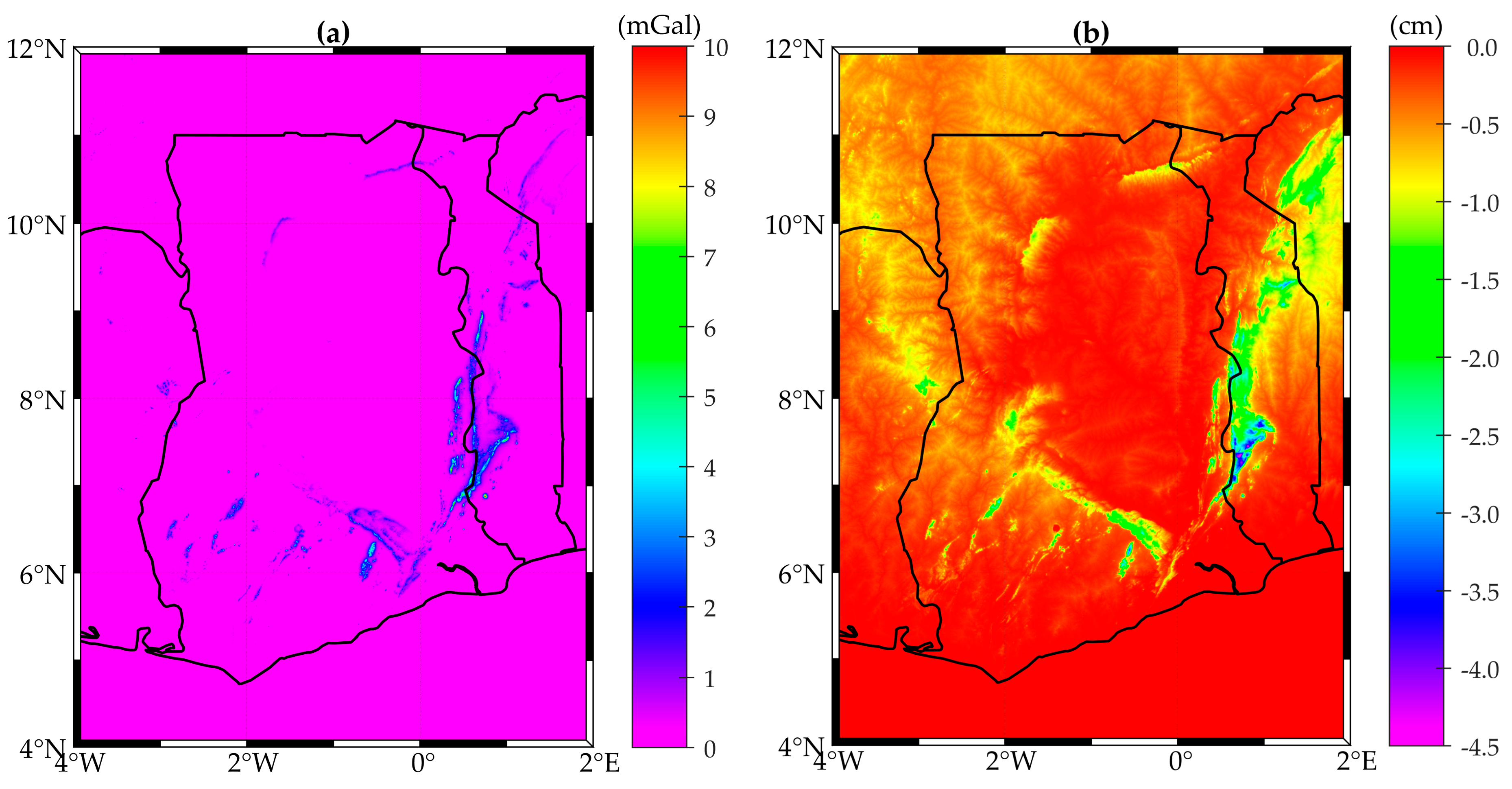
We use the 30 arc-second SRTM30_PLUS topography and bathymetry DEM [21] as input data for the computation of topography-generated gravity field quantities over the region bounded by 4° W and 2° E longitude, 4° N and 12° N latitude. Panels (a) and (b) of Figure 1 show that the values for the terrain corrections and indirect effect, respectively, are very small, reemphasizing the relatively low-lying terrain of the study area, with the regions of Ghana housing mountains having the highest amplitudes.
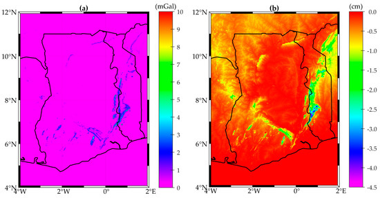
Figure 1.
Topography-generated gravity field quantities for the study area computed using SRTM30_PLUS topography/bathymetry; (a) Terrain correction computed using SRTM30_PLUS topography/bathymetry data as input for Equation (17); and (b) Indirect effect computed using Equation (18).
3. Numerical Results and Discussion
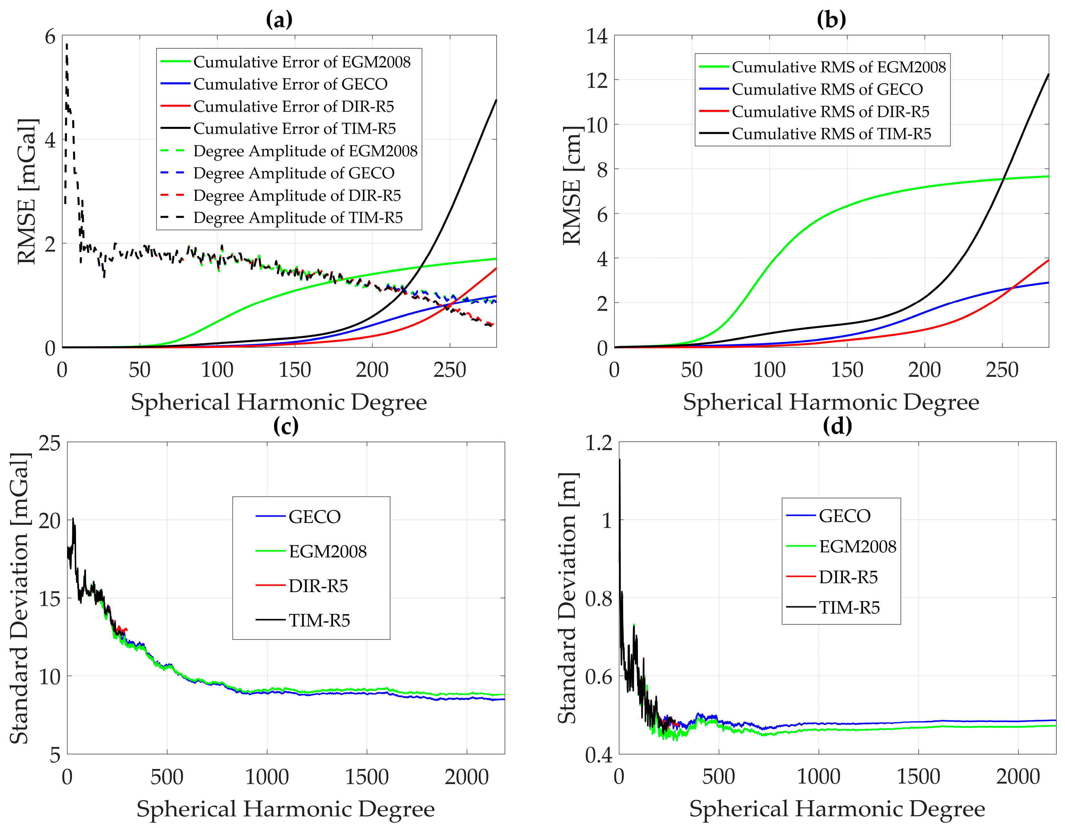
Figure 2 panels (a) and (b) show the global inter-comparison of the tested GGMs computed from Equation (3). GECO has the smallest cumulative errors both in terms of geoid heights and gravity anomaly while TIM-R5 has the worst root-mean-square of the errors (RMSEs). Notice that with the exception of TIM-R5, all the other models have gravity anomaly RMSEs below 2 mGal. It is worth noting that while this may appear to be a good metric for the selection of a GGM for geoid computation, it is not advised since such a comparison does not take into account the effect of (local) terrestrial data, which are used for geoid computation and thus, contribute to the accuracy of the geoid.
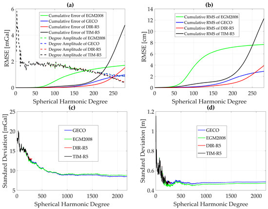
Figure 2.
GGM inter-comparison and comparison with terrestrial data. The dashed lines in panels (a) and (b) are the cumulative RMSEs, while the solid lines represent the degree amplitudes. (a) Inter-comparison of GGMs based on gravity anomaly; (b) Inter-comparison of GGMs based on geoid heights; (c) Comparison of terrestrial gravity anomaly and gravity anomalies computed from GGM; (d) Comparison of GPS/trigonometric heights with GGM geoid undulations.
In contrast, the panels (c) and (d) of Figure 2 display the results of the standard deviation of the differences between gravity anomalies from terrestrial data and GGM (see panel (c) of Figure 2), and geoid heights from terrestrial data and GGM (panel (d) of Figure 2). We have found that beyond d/o 234 and 222 (see panels (c) and (d) of Figure 2), where the smallest standard deviations are recorded for gravity anomalies and geoid heights, respectively, very little signal change occurs. Thus, these have been chosen as the best performing d/o, corresponding to gravity anomalies and geoid heights, respectively. In addition, EGM2008 gives the smallest standard deviation in both cases (see panels (c) and (d) of Figure 2). Figure 2c shows EGM2008 and GECO with smaller standard deviations than TIM-R5 and DIR-R5 showing agreement with the results of the cumulative anomaly degree variances, obtained using Equation (3) for gravity anomalies (panel (a) Figure 2). One may be tempted to use such a comparison in the selection of a GGM for geoid computation. However, since this approach does not take into account the differences in frequencies between terrestrial data and GGM, it may present a bias in the results and is thus not a good metric for the comparison of terrestrial data and GGMs.
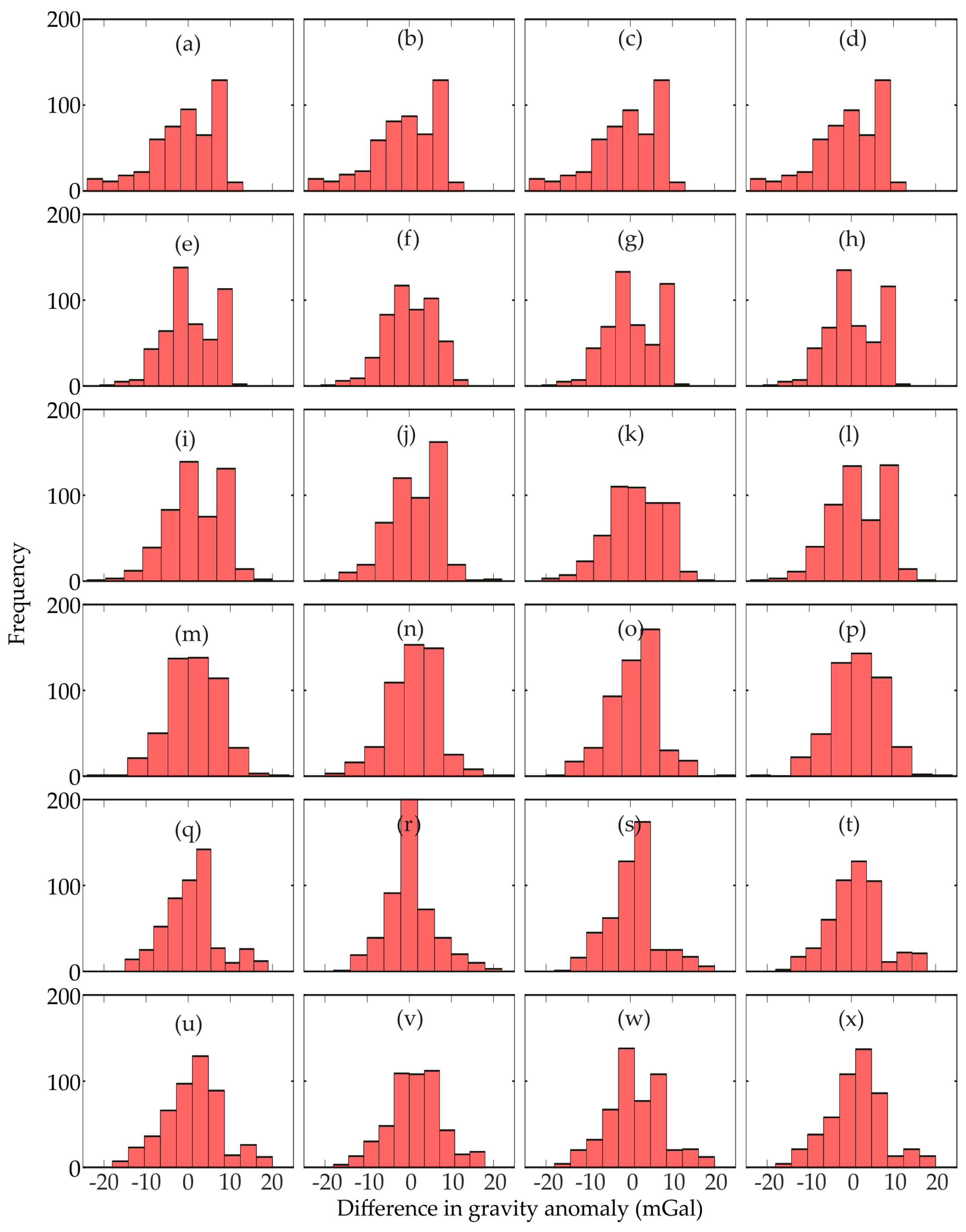
The Gaussian averaging function aims to filter terrestrial data for comparison with global models. The averaging process requires taking the mean of gravity anomalies within a certain radius, which is a function of the degree of expansion (). We have compared averaged free-air gravity anomalies with gravity anomalies computed from DIR-R5, EGM2008, GECO and TIM-R5 at d/o 90, 150, 200, 222, 234, and 250 (see Figure 3). Recall that the direct comparison of terrestrial and satellite gravity data (see panels (c) and (d) of Figure 2) does not take into consideration the varying frequencies, or as it were, assumes that the terrestrial data and satellite data have the same frequencies. Since this is not the case, such a comparison may present a bias. Thus, the Gaussian averaging function may prove a better method for the comparison and selection of an optimal global model and d/o.
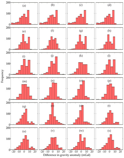
Figure 3.
Comparison between filtered gravity anomalies and GGM anomalies in mGal. Each row represents a degree and order (d/o) of expansion, where row 1 (panels a–d) shows the values for d/o 90, row 2 (panels e–h) shows the values for d/o 150, row 3 (panels i–l) shows the values for d/o 200, row 4 (panels m–p) shows the values for d/o 222, row 5 (panels q–t) shows the values for d/o 234, and row 6 (panels u–x) shows the values for d/o 250. The columns represent the tested models arranged from left to right as DIR-R5, EGM2008, GECO, and TIM-R5, respectively.
We have decided to select the coordinates of the smoothed gravity anomalies to coincide with the coordinates of the original data points as opposed to grid knots, as used in reference [5]. This decision was partly influenced by the likelihood of errors arising from resampling the original data into a grid. Nevertheless, one may circumvent the problem of interpolation errors (when grids are used) by treating the GGM anomalies in exactly the same way as the ground-based anomalies. That is, GGM gravity anomalies should be computed at the original data points and then gridded. This way, any interpolation errors will be canceled out because of differencing. Notwithstanding, we note that care should be taken in using grids as it may result in biased error estimates, particularly in cases where data is scanty (and is slightly time-consuming).
Although the standard deviations for the different GGMs are quite close for the d/o under consideration, EGM2008 recorded the smallest standard deviations for all d/o, while GECO came second in most of the d/o except 150 and 250 (Figure 3). DIR-R5 recorded the worst performances for all d/o except 150 (see Table 1).

Table 1.
Standard deviation of the smoothing process (mGal).
It should be noted that with the exception of EGM2008, the GGMs recorded better standard deviations at d/o 150 than at 222. Needless to say, the differences between the standard deviations of the two-aforementioned d/o are small with negligible geoid error differences, i.e., the differences between their error contribution to the geoid. For example, the effect of the difference between the standard deviations of DIR-R5 at d/o 150 and 222 is a geoid error of 1.53 cm for an integration radius of 100 km and latitudes 2° N, 6° N and 12° N, see Equation (2-433) of Ref. [1] (p. 127). Obviously, for the computation of a centimeter-level accuracy, such a difference is significant.
Generally, lower degrees of truncation are preferred to match low resolution terrestrial gravity data. However, it has been shown here that a degree and order must be carefully chosen to avoid the risk of introducing larger errors. For example, the geoid error for a standard deviation of 7.907 mGal for DIR-R5 at d/o 90 for an integration radius of 100 km and a latitude of 2° N is 80.8 cm and 61.1 cm for a standard deviation of 5.975 mGal corresponding to d/o 222, a difference of almost 20 cm.
Clearly, these large errors suggest a poor quality of the terrestrial data, rather than the Gaussian averaging function. It goes to emphasize why a precise geoid is presently impossible for Ghana and why this work is important to provide an improved gravimetric geoid model.
Next, we compute gravimetric geoid models for all the GGMs and the degrees and orders using Heck and Grüninger’s modification, e.g., [18] on a 5′ × 5′ grid. For the computation of the zero-degree term, we use 62,636,856.00 m2·s−2 and 62,636,851.7146 m2 s−2 as the potentials on the geoid and WGS 84 ellipsoid [1,22]. We validate these geoid models by first comparing them with 11 GPS/trigonometric data in what is known as absolute validation, where the geoid heights from the gravimetric geoid are compared with geometric geoid heights from GPS/trigonometric data .
The statistics of this comparison in Table 2 shows EGM2008 to be the best performing GGM for the investigated d/o. In addition, the d/o 222 recorded the smallest standard deviations for all the GGMs. As was expected, the d/o 90 gave the largest standard deviation reiterating the importance of a carefully chosen degree and order over an assumed selection of a smaller d/o to match the resolution of terrestrial data.
Table 2.
Statistics of absolute validation of gravimetric geoid models using GPS/trigonometric data (m).
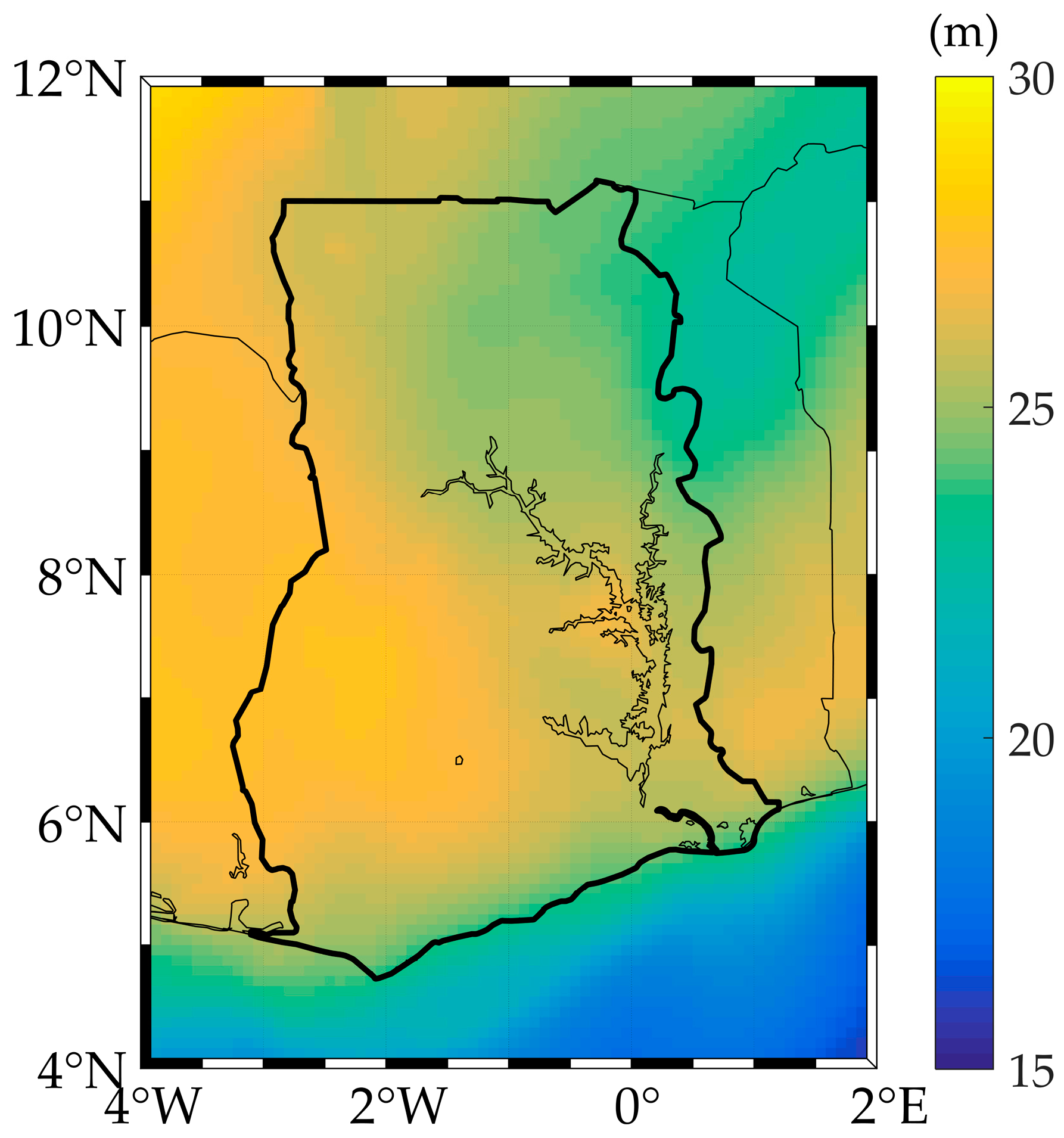
In comparison to the previous geoid [6], with a standard deviation of almost 50 cm (0.497 m), the geoid models computed at the tested d/o except d/o 90 in this work are an improvement. Selecting EGM2008 at degree 222 (Figure 4) gives an improvement of 8%, while the best performing satellite-only model, TIM-R5, gives a 6% improvement at the same d/o.
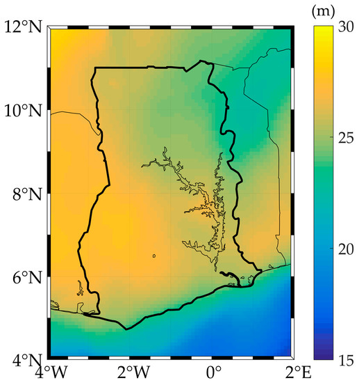
Figure 4.
Gravimetric geoid model computed using EGM2008 up to degree and order 222.
Next, we carried out a relative validation of the gravimetric geoid models (Table 3). This allows for a sense of the measure of errors per km of leveling line. Given two points, A and B, on the surface of the Earth at a distance apart, the relative error is expressed in units of mm for every kilometer as:
Table 3.
Statistics of relative validation of gravimetric geoid models using Equation (19). All values are in meters.
To determine whether a leveling survey is acceptable, misclosures are compared with permissible values on the basis of either number of setups or distance covered. Generally, the allowable misclosure is given, in terms of distance as , where C is the allowable loop or section misclosure in millimeters, is a constant and the total length leveled in kilometers. Values for the constant may be 4, 5, 6, 8, and 12 mm for five classes of leveling specified as first-order class I, first-order class II, second-order class I, second-order class II, and third-order, respectively, as proposed by the Federal Geodetic Control Subcommittee (FGCS) of USA.
EGM2008 again gives the best performance with the smallest error at d/o 222. Thus, one is expected to record an error of ±6.8 mm for every kilometer of leveling and for distances ranging from 20 to 225 km, corresponding to the minimum and maximum distances, respectively, between the GPS/trigonometric stations. It should be noted that the mean value of the errors for all models for d/o 222 meet the 8-mm level tolerance for second-order class II leveling.
4. Conclusions
We have shown in this study the importance of using a method for carefully selecting a GGM, degree and order for the computation of a gravimetric geoid model in the RCR technique. We showed that because terrestrial gravity anomalies and gravity anomalies computed from GGMs have different wavelengths, a direct comparison might introduce biases. Thus, we suggested the extension of the Gaussian averaging function, which takes into account the different frequencies of terrestrial and GGM data for the selection of a degree and order and GGM for the long wavelength contribution in the RCR technique. EGM2008 gave the best performance at all degrees and orders.
We verified the results from the Gaussian averaging function by computing geoid models and comparing them with GPS/trigonometric data for the study area. The degree and order 222 was chosen as the optimal, resulting in an improved geoid model over the previous gravimetric geoid. The EGM2008 geoid recorded a standard deviation of 0.457 m, an 8% improvement over the previous model.
A relative validation of the geoid models reemphasized that the degree and order 222 and EGM2008 were the optimal d/o and GGM. The d/o 222 EGM2008 gravimetric geoid model may be used to replace second-order class II leveling for baselines between 20 and 225 km with an expected error of 6.8 mm for every kilometer of the leveling line.
It is clear that while the quality of the terrestrial gravity data is low, an informed computation of a gravimetric geoid model, e.g., the careful selection of an optimal GGM and degree of truncation, will give improved results. The d/o 222 EGM2008 geoid has been named the Ghanaian Gravimetric Geoid 2017 (GGG 2017), and is available for the general user community through the geoid model repository of the International Service for the Geoid (IGS) at http://www.isgeoid.polimi.it/.
Acknowledgments
This work was done as part of a Master’s thesis at Hohai University, China. We thank the Jasmine Jiangsu Government Scholarship Secretariat for providing funding for this period. We also wish to thank John Ayer of the Kwame Nkrumah University of Science and Technology, Ghana, for providing GPS/trigonometric heights. Finally, we express appreciation to the Bureau Gravimétrique International (BGI) for providing additional terrestrial gravity data and marine gravity anomalies and to the International Centre for Global Earth Models (ICGEM) for making GGM data freely accessible.
Author Contributions
Caleb I. Yakubu conceived, designed, and performed the experiments; Caleb I. Yakubu, Vagner G. Ferreira, and Cosmas Y. Asante analyzed the data and wrote the paper.
Conflicts of Interest
The authors declare no conflict of interest.
References
- Hofmann-Wellenhof, B.; Moritz, H. Physical Geodesy, 2nd ed.; Springer: Berlin, Germany, 2006; p. 413. [Google Scholar]
- Hirt, C.; Featherstone, W.E.; Marti, U. Combining EGM2008 and SRTM/DTM2006.0 residual terrain model data to improve quasigeoid computations in mountainous areas devoid of gravity data. J. Geod. 2010, 84, 557–567. [Google Scholar] [CrossRef]
- Jekeli, C. Alternative Methods to Smooth the Earth’s Gravity Field; Technical Report 327; Ohio State University: Columbus, OH, USA, 1981; p. 54. [Google Scholar]
- Huang, J.; Véronneau, M.; Mainville, A. Assessment of systematic errors in the surface gravity anomalies over North America using the GRACE gravity model. Geophys. J. Int. 2008, 175, 46–54. [Google Scholar] [CrossRef]
- Bomfim, E.P.; Braitenberg, C.; Molina, E.C. Mutual evaluation of global gravity models (EGM2008 and GOCE) and terrestrial data in Amazon basin, Brazil. Geophys. J. Int. 2013, 195, 870–882. [Google Scholar] [CrossRef]
- Klu, A.M. Determination of a Geoid Model for Ghana Using the Stokes-Helmert Method. Master’s Thesis, University of New Brunswick, Saint John, NB, Canada, 2015. [Google Scholar]
- Davis, P. Gravity Survey of Ghana; State Publishing Corporation (Printing Division): Accra, Ghana, 1962; p. 250. [Google Scholar]
- Mäkinen, J.; Ihde, J. The permanent tide in height systems. In Observing Our Changing Earth; Sideris, M.G., Ed.; Springer: Berlin/Heidelberg, Germany, 2009; pp. 81–87. [Google Scholar]
- Ekman, M. Impacts of geodynamic phenomena on systems for height and gravity. Bull. Géodésique 1989, 63, 281–296. [Google Scholar] [CrossRef]
- Tenzer, R.; Vatrt, V.; Abdalla, A.; Dayoub, N. Assessment of the LVD offsets for the normal-orthometric heights and different permanent tide systems—A case study of New Zealand. Appl. Geomat. 2011, 3, 1–8. [Google Scholar] [CrossRef]
- Pail, R.; Bruinsma, S.; Migliaccio, F.; Förste, C.; Goiginger, H.; Schuh, W.-D.; Höck, E.; Reguzzoni, M.; Brockmann, J.M.; Abrikosov, O.; et al. First GOCE gravity field models derived by three different approaches. J. Geod. 2011, 85, 819–843. [Google Scholar] [CrossRef]
- Bruinsma, S.L.; Förste, C.; Abrikosov, O.; Marty, J.-C.; Rio, M.-H.; Mulet, S.; Bonvalot, S. The new ESA satellite-only gravity field model via the direct approach. Geophys. Res. Lett. 2013, 40, 3607–3612. [Google Scholar] [CrossRef]
- Pavlis, N.K.; Holmes, S.A.; Kenyon, S.C.; Factor, J.K. The development and evaluation of the Earth Gravitational Model 2008 (EGM2008). J. Geophys. Res. Solid Earth 2012, 117. [Google Scholar] [CrossRef]
- Ustun, A.; Abbak, R.A. On global and regional spectral evaluation of global geopotential models. J. Geophys. Eng. 2010, 7, 369–379. [Google Scholar] [CrossRef]
- Gilardoni, M.; Reguzzoni, M.; Sampietro, D. GECO: A global gravity model by locally combining GOCE data and EGM2008. Stud. Geophys. Geod. 2016, 60, 228–247. [Google Scholar] [CrossRef]
- Wahr, J.; Molenaar, M.; Bryan, F. Time variability of the earth’s gravity field: Hydrological and oceanic effects and their possible detection using GRACE. J. Geophys. Res. Solid Earth 1998, 103, 30205–30229. [Google Scholar] [CrossRef]
- Torge, W.; Müller, J. Geodesy, 4th ed.; Walter de Gruyter: Berlin, Germany, 2012; p. 445. [Google Scholar]
- Ferreira, V.G.; Zhang, Y.; de Freitas, S.R.C. Validation of GOCE gravity field models using GPS-leveling data and EGM08: A case study in Brazil. J. Geod. Sci. 2013, 3, 209–218. [Google Scholar] [CrossRef]
- Featherstone, W.E. Software for computing five existing types of deterministically modified integration kernel for gravimetric geoid determination. Comput. Geosci. 2003, 29, 183–193. [Google Scholar] [CrossRef]
- Wichiencharoen, C. The Indirect Effects on the Computation of Geoid Undulations; The Ohio State University: Columbus, OH, USA, 1982; Volume 336, p. 104. [Google Scholar]
- Becker, J.J.; Sandwell, D.T.; Smith, W.H.F.; Braud, J.; Binder, B.; Depner, J.; Fabre, D.; Factor, J.; Ingalls, S.; Kim, S.-H.; et al. Global bathymetry and elevation data at 30 arc seconds resolution: SRTM30_plus. Mar. Geod. 2009, 32, 355–371. [Google Scholar] [CrossRef]
- Ferreira, V.G.; de Freitas, S.R.C.; Heck, B. Analysis of the discrepancies between the Brazilian vertical reference frame and GOCE-based geopotential model. In International Association of Geodesy Symposia; International Association of Geodesy: Munich, Germany, 2016; Volume 12, pp. 227–232. [Google Scholar]
© 2017 by the authors. Licensee MDPI, Basel, Switzerland. This article is an open access article distributed under the terms and conditions of the Creative Commons Attribution (CC BY) license (http://creativecommons.org/licenses/by/4.0/).