Article

Glacier Snowline Determination from Terrestrial Laser Scanning Intensity Data

1
Institute of Geography, University of Innsbruck, 6020 Innsbruck, Austria
2
Institute of Atmospheric and Cryospheric Sciences, University of Innsbruck, 6020 Innsbruck, Austria
3
Department of Geography, University of Zurich, 8006 Zurich, Switzerland
*
Author to whom correspondence should be addressed.
Geosciences 2017, 7(3), 60; https://doi.org/10.3390/geosciences7030060
Submission received: 29 April 2017 / Revised: 28 June 2017 / Accepted: 10 July 2017 / Published: 17 July 2017
(This article belongs to the Special Issue Cryosphere)

Abstract

:
Accurately identifying the extent of surface snow cover on glaciers is important for extrapolating end of year mass balance measurements, constraining the glacier surface radiative energy balance and evaluating model simulations of snow cover. Here, we use auxiliary information from Riegl VZ-6000 Terrestrial Laser Scanner (TLS) return signals to accurately map the snow cover over a glacier throughout an ablation season. Three classification systems were compared, and we find that supervised classification based on TLS signal intensity alone is outperformed by a rule-based classification employing intensity, surface roughness and an associated optical image, which achieves classification accuracy of 68–100%. The TLS intensity signal shows no meaningful relationship with surface or bulk snow density. Finally, we have also compared our Snow Line Altitude (SLA) derived from TLS with SLA derived from the model output, as well as one Landsat image. The results of the model output track the SLA from TLS well, however with a positive bias. In contrast, automatic Landsat-derived SLA slightly underestimates the SLA from TLS. To conclude, we demonstrate that the snow cover extent can be mapped successfully using TLS, although the snow mass remains elusive.

1. Introduction

Determinations of glacier mass balance, which is the change of the mass of a glacier over a unit of time, provide a key metric for monitoring glacier changes and their relationship with the forcing climate conditions and hydrological impacts. The mass balance time series of 30 ‘benchmark’ glaciers (e.g., [1,2]) provides the basis for reconstructing past contributions to sea level rise [3,4,5,6], for extrapolating glaciers’ contribution to regional water supply (e.g., [7]) and for glacier change detection, attribution [8,9] and projection studies (e.g., [4,10,11,12,13]). Uncertainties of direct glaciological mass balance measurements are usually dominated by uncertainties in accurately determining snow mass accumulation (e.g., [14,15]). This is partly because the accumulation area is sometimes less accessible than the lower part of the glacier, so fewer measurements are made, but is also because the snow cover distribution, and Snow Water Equivalent (SWE), vary substantially in space and time over a glacier surface as a function of factors such as: initial distribution, avalanches, wind-blown snow, effects of shadowing and preferential ablation locations. Accurate knowledge of snow cover and SWE distribution is valuable for (i) extrapolating from point measurements used in deriving the mass balance of a glacier [16,17], (ii) evaluating the performance of spatially-distributed Surface Energy Balance (SEB) models used to simulate the glacier mass balance [18], (iii) determining the albedo distributions for surface energy balance modelling and (iv) determining transient and end of season snow line altitudes, which are useful glaciological metrics for approximating glacier mass balance and glacier mass change [19].
In the classical glaciological method, snow distribution over a glacier is typically determined on the basis of a number of point field observations extrapolated over the glacier surface. Furthermore, snow density is generally determined at only a single or very few sites on the glacier, and the potentially important spatial distribution of snow density remains unknown [2,20].
Remote sensing methods developed over recent decades have the potential to provide accurate high resolution observations for glacier monitoring. In particular, the use of laser scanning, also referred to as LiDAR (Light Detection and Ranging) or LADAR (Laser Detection and Ranging), which can be applied from the air or the ground [21], represents a step change in the capacity to generate high resolution topographic data over large areas and has become widely used for glaciological applications [22]. Both Airborne (ALS) and Terrestrial Laser Scanning (TLS) are increasingly used for detecting changes in glacier volume and dynamics [23,24]. TLS-derived Digital Terrain Models (DTMs) are useful for studying small-scale processes and are of sufficiently high quality for evaluating the spatial distribution of measurements and modelling over the glacier surface. Previous studies have successfully demonstrated the usefulness of TLS for monitoring the behavior and surface changes of glaciers, rock glaciers, geohazards and snow cover [25,26,27,28,29,30,31,32,33,34,35]. The limitations of a the TLS scan quality and resolution are related to the range of the laser, the scan rate, the availability of suitable scanning positions in regards to obtaining high angle view points for the DTM subject and the inclusion of stable ground control points for co-registration of repeat scans for change detection. In addition to the xyz information, LiDAR sensors offer intensity data from each returned laser point, and some systems also offer simultaneous optical imagery. The intensity is the recorded return signal strength defined by the amount of backscattered energy [27,28,36,37]. Jörg et al. [38] and Fritzmann et al. [39] demonstrated the potential of using intensity data for surface classification using ALS data over a high mountain area, including a glacier. On this basis, we propose two hypotheses that the intensity from a high resolution TLS scan can be used (i) as a tool for accurately mapping the snow covered area of a glacier based on differences in the backscattered energy of snow and ice and (ii) as an indicator of snow density based on the fact that low density, fresh and unmetamorphosed snow is expected to return a greater signal strength than older, denser snow.
To test these hypotheses, we develop a glacier surface classification based on TLS intensity data and determine the utility of such a classification for accurately mapping the snow cover distribution over the glacier surface and its change over time. A comparison of in situ snow density measurements and TLS intensity values is applied to investigate whether spatially-distributed density approximations can be made from TLS intensity maps. Finally, snowline approximations based on the TLS surface classification are compared with those based on a hydrological model and on Landsat data. Together, these analyses explore the utility of TLS intensity for generating more accurate extrapolations of point glacier measurements and for generating datasets against which the performance of distributed numerical models can be evaluated.

2. Materials and Methods

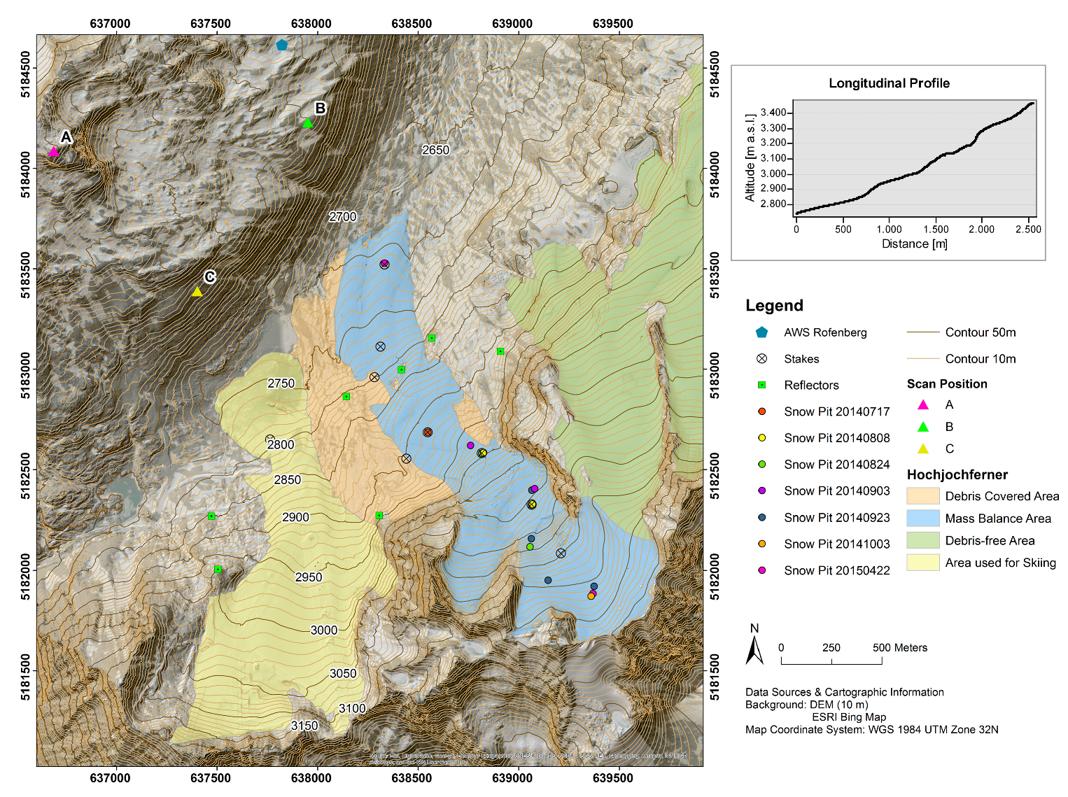
2.1. The Study Site: Hochjochferner

The study glacier, Hochjochferner (46°46.9′ N, 10°48.9′ E), is located in the Rofental, a high mountain valley in the upper Ötztal, Austria. In 2013, the glacier covered an area of about 5.3 km2 and has retreated from its Little Ice Age maximum to form four separate areas (see Figure 1), the westernmost of which hosts a skiing resort and is separated from the mass balance area by a debris-covered area. The mass balance area is the part monitored in this study and for simplification referred to as Hochjochferner (HJF).
Based on ALS data acquired from the Tyrolean Government [40] in 2013, this study unit of HJF was determined from the DEM, and HJF covered ca. 1 km2 with a flowline length of ca. 2.5 km at that time. Its altitude ranges from 3515 m (top of Fineilspitze) down to 2700 m. The glacier is exposed to the north and northeast and has a relatively flat terminus; the average slope of HJF is 18°. In the mass balance year of 2013/2014, the glacier mass balance was measured from a limited number of glaciological measurements and was found to be −244 kg m−2, with an Equilibrium-Line Altitude (ELA) of 3055 m a.s.l.
In 2006, HJF contributed to the Rofenache River catchment (Rofental), which covers ca. 98 km2, of which 35% is glaciated [41]. The Rofental is an inner alpine valley with relatively low annual precipitation due to rain shadow effects [42]. Snow cover is typically present from November–April in the lower parts and until the end of June in the higher parts [43], and 44% of the annual runoff is nival [44]. Mean annual air temperature in the village of Vent (46°51.5′ N, 10°54.7′ E), 1898 m a.s.l. ca. 10 km southwest from the study area, is reported as 2.8 °C for the period 1982–2011 [45], and mean annual precipitation (measured with totalizing rain gauges over the period 1982–2003) is reported as ca. 797 mm in Vent, increasing to 1072 mm at the Rofenberg (46°48.5′ N, 10°47.6′ E) at 2827 m on the opposite slope of Hochjochferner [46]. Recent data from weather stations located in Vent and Rofenberg are shown in Table 1. The data indicate that conditions over the recent period were significantly warmer and slightly wetter than the longer term average over these periods. Unfortunately, there is a data gap in the air temperature measurements in July 2014, and therefore, the air temperature is calculated with and without (in brackets) the data gap.

2.2. TLS-Acquisition

A Riegl VZ-6000 scanner [49] was used to perform nine surface scans of the studied part of HJF during the mass balance (hydrological) years of 2014 and 2015, capturing the surface at the beginning and end of both mass balance years and multiple times throughout the summer ablation season of 2014. This scanner emits near-infrared laser pulses with a wavelength of 1064 nm, which is suitable for recording reflections from ice, snow and firn, even at high distances, and has a built-in optical camera [49] (Table 2). The laser pulse repetition rate was set to 30 kHz to allow a maximum range with an angular step width of 0.005°. With this setting, a point spacing of approximately 0.09 m at 1 km is possible. Air temperature, humidity and pressure conditions at the TLS site during each scan were measured using a hand-held Kestrel 6000 weather meter and input into the Riegl system, which then performs automatic correction for these atmospheric conditions.
The TLS stores the measurement data file containing the raw coordinates, the signal amplitude and reflectance (the intensity), scanning angles theta and phi, along with a corresponding preview data file, a preview picture file and camera image files [49]. Scans of HJF were carried out from three positions to achieve maximum coverage, and the positions of seven 0.3 × 0.3 m metal reflectors mounted on rock or bedrock in the field of view were surveyed to geodetic accuracy to facilitate the most accurate co-registration of surface scans [34]. Three of the Ground Control Points (GCP) are located on newly-outcropping bedrock within the 2013 outline of the glacier. These location were identified as bedrock outcrops rather than large boulders embedded in the ice on the basis of their sheer size and indications of being geologically consistent with the exposed bedrock flanking the glacier. The details of the scan campaigns are given in Table 3. The GCP locations were surveyed with a horizontal accuracy of 0.04 m or better.

2.3. TLS Processing

Raw TLS data were pre-processed with RiSCAN PRO® software (Riegl Laser Measurement Systems, Horn, Austria). In seven of nine scan campaigns, three scan positions were used. On two scanning dates, the weather conditions were only good in the morning, and therefore, the time was sufficient for two scans. Photos from the inbuilt camera are imported and merged with the point cloud prior to georeferencing so that these images are also georeferenced in a subsequent step. Georeferencing was performed on the basis of the GCP targets where visible and otherwise on the relative orientation to the merged georeferenced scans from 18 July 2014. Since most of the reflectors were detected during this scan campaign, the highest coverage of the area was achieved, and the scan positions were measured with a Trimble R6 GPS (Trimble, Sunnyvale, CA, USA). For this, scans were initially manually aligned to the georeferenced scan from 18 July 2014 using the Coarse Registration tool, before applying an automated Multi Station Adjustment in RiSCAN PRO (Riegl). The mean vertical accuracy of this co-registration procedure is between 0.03 and 0.04 m. Finally, each scan was combined into one point cloud and exported for further analysis.
Surface roughness was computed on the point clouds using tools within the Laserdata Information System (LIS) software developed by Laserdata GmbH (Innsbruck, Austria) and embedded in the open source SAGA GIS [50]. Subsequent analyses and classifications were performed once point clouds were converted to grids with a simple point cloud to grid tool because analyses on raster layers are usually faster and easier to perform than point cloud analysis (e.g., [51,52]). The new raster layers have a resolution of 1 × 1 m, and each grid cell value is based on the mean of 8–15 points.

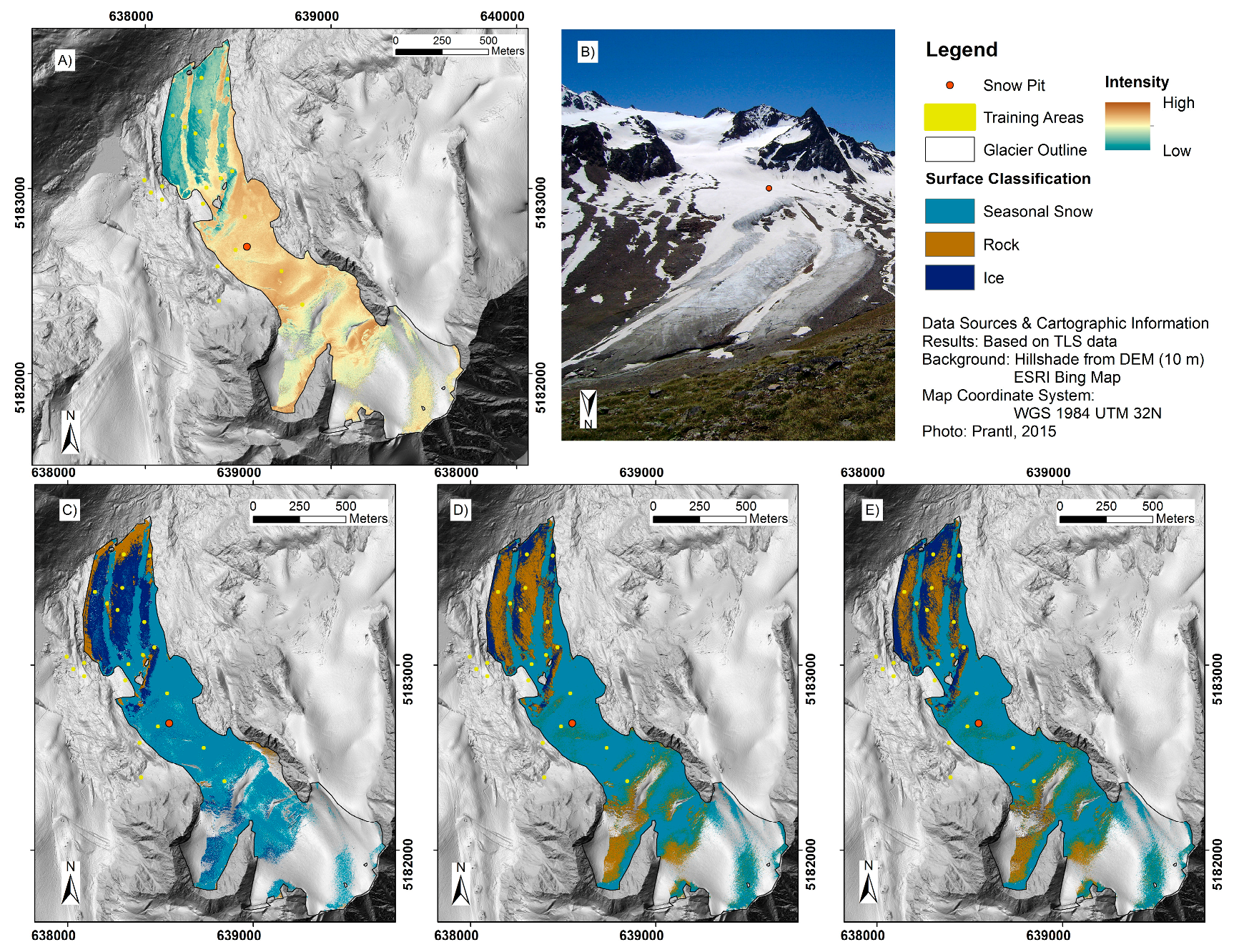
2.4. Surface Classification

The TLS is capturing the backscattered intensity, which records the surface reflecting information. The amount of backscattered energy recorded by the TLS is referred to as the signal intensity [37] expressed as [53]:
P r = P t D r 2 R 4 β t 2 ρ A s
where Pr refers to the received power, Pt to the transmitted power, Dr to the aperture size of the receiver, R to the range, β to the beam divergence, Ω to the reflectivity of the target, ρ to the scattering and As to the receiving area of the scatter. The equation shows that the signal intensity depends on the scanning geometry, as well as the surface type, surface properties, instrumental parameters and atmospheric conditions [21,54,55,56,57,58,59,60,61]. The VZ-6000 laser scanner corrects the intensity automatically and stores the intensity values as reflectance.
Surface classification, whereby all pixels of an image are classified into a finite number of categories or surface classes, is commonly performed on the basis of reflectance properties [62]. After specification of the desired classes, training areas are manually set, the signatures of the training areas are extracted, and the image is classified on the basis of these surface signatures. For this study, the most common surface types occurring in the study area were identified for classification: seasonal snow, rock and ice. Training areas for these surface types were manually identified for each scan and scanning date on the basis of field photos and observations from the field log book. Three types of classification procedures were tested: two supervised classifications based on: (i) Maximum Likelihood (MLC); (ii) Minimum Distance (MDC); and (iii) a Rule-Based Classification (RBC). The supervised classification procedures rely on the TLS intensity signal alone, whereas the rule-based classification additionally uses photos from the built-in camera and surface roughness calculated from the point cloud.
In the supervised classification, the user determines the number of desired classes and then identifies training areas for spectral response patterns. Then, the image is classified on a pixel by pixel basis by comparing each unknown pixel to the characteristics of different classes and assigned into the most similar category. It is considered suitable when there are relatively few desired classes and there is high confidence in the training areas, as is the case with this study.
The MLC is the most popular supervised classification method. This technique is based on probability density functions. The density is determined from the center of each training area. The probability of a pixel belonging to each identified class is calculated, and then, it is assigned to the class with the highest probability. Therefore, a sufficient number of pixels of each class is required. Richard and Jia [63] give the equation for each pixel as:
g k ( x ) = ln p ( C k ) 1 2   ln |   k   | 1 2 ( x y k ) t k 1 ( x y k )
where Ck is the land cover class k, x is the spectral signature vector of an image pixel, p(Ck) is the probability that the correct class is Ck, ∣∑k∣ is the determinant of the covariance matrix of the data in class Ck, k 1   is the inverse of the covariance matrix and yk is the spectral signature vector of class k.
The MDC is one of the simpler classification systems. In the first step, the mean value of each class is calculated. Then, the (mostly Euclidean) distance between one unknown pixel in n directions is determined and classified into the category with the shortest distance, based on following equation:
d ( x , y ) =   i = 1 n ( x i y i ) 2
where x is the spectral signature vector of an image pixel, y is the spectral signature vector of a training area and n is the number of image bands [64]. A disadvantage is that the algorithm assumes that spectral variability is the same in all direction, which is not always the case.
The RBC is a hierarchically-based classifier, which describes a set of decision rules (decision tree) or just a single rule. It is also based on a pixel-by-pixel method, and information from additional data can be taken into account. A rule-based classification determines the thresholds of the desired image classes, and the pixels are reclassified according to these thresholds. This method is very effective, has a very low percentage of statistical errors [39,65,66] and needs less computing time than maximum likelihood classification.
The accuracy of each classification was determined empirically, by calculating the confusion and error matrices. The confusion matrix compares information from the reference data, often called ground truth data, to sampled areas of the classified image; thus, the performance assessment indicates how well the statistics extracted from these areas can be used to categorize the same area [65]. For each class (seasonal snow, rocks and ice), seven polygons, with a size of 4 × 4 m, are identified using photos from the field campaigns and field log books from the day before scanning the glacier, as well as photos from the inbuilt laser scanner camera of the same day as the glacier was scanned and used as the reference data for the accuracy assessment. Then, the intensity values of each polygon were extracted and further analyzed. Thereby, the percentage of pixels from each class in the raster grid classified correctly by the classifying algorithm can be estimated, and the actual and predicted classifications by the classification system are expressed [65]. An error matrix calculates the Overall Accuracy (OAA), the User’s Accuracy (UA) and the Producer’s Accuracy (PA). OAA is computed by summing the major diagonal (i.e., the correctly-classified pixels) and dividing by the total number of classified pixels. To determine UA, the number of correctly-classified pixels in each class is divided by the total number of pixels that were classified in that class (the row total). The PA is calculated by dividing the number of correctly-classified pixels in each class by the number of reference pixels used in this class (the column total). Both calculations (UA and PA) represent individual class accuracies. UA indicates the probability for which a pixel in a given class actually represents the surface class on the ground, and PA measures how well the reference pixels of a surface class are classified by the program. It should be considered that if the results of the error matrix are good, it means nothing more than that the reference areas are homogenous, spectrally separable and that the classification method performs well in these areas. It indicates little about how the classification system works elsewhere in the investigated area [65,67].

2.5. Relationship between TLS Intensity and Snow Density

To determine whether TLS intensity values can be used as an indicator of snow density, simple correlation was performed between the intensity values in the pixel nearest each snow pit and the in situ snow density measurements, both (i) the depth-averaged snow density in the pit and (ii) the density of the uppermost sample. The correlation coefficient r is calculated using following equation:
r = 1 n 1 i = 1 n ( x i x ¯ s x ) ( y i y ¯ s y )
where the number of data points is given by n, the data points are represented by xi and yi, the mean of xi is x ¯ , the standard deviation of xi is denoted by sx, the mean of yi is y ¯ and the standard deviation of yi is denoted by sy. The correlation coefficient has a value range between −1 and +1. A strong correlation has a value higher than ±0.7 and a moderate correlation higher than ±0.4 [68].

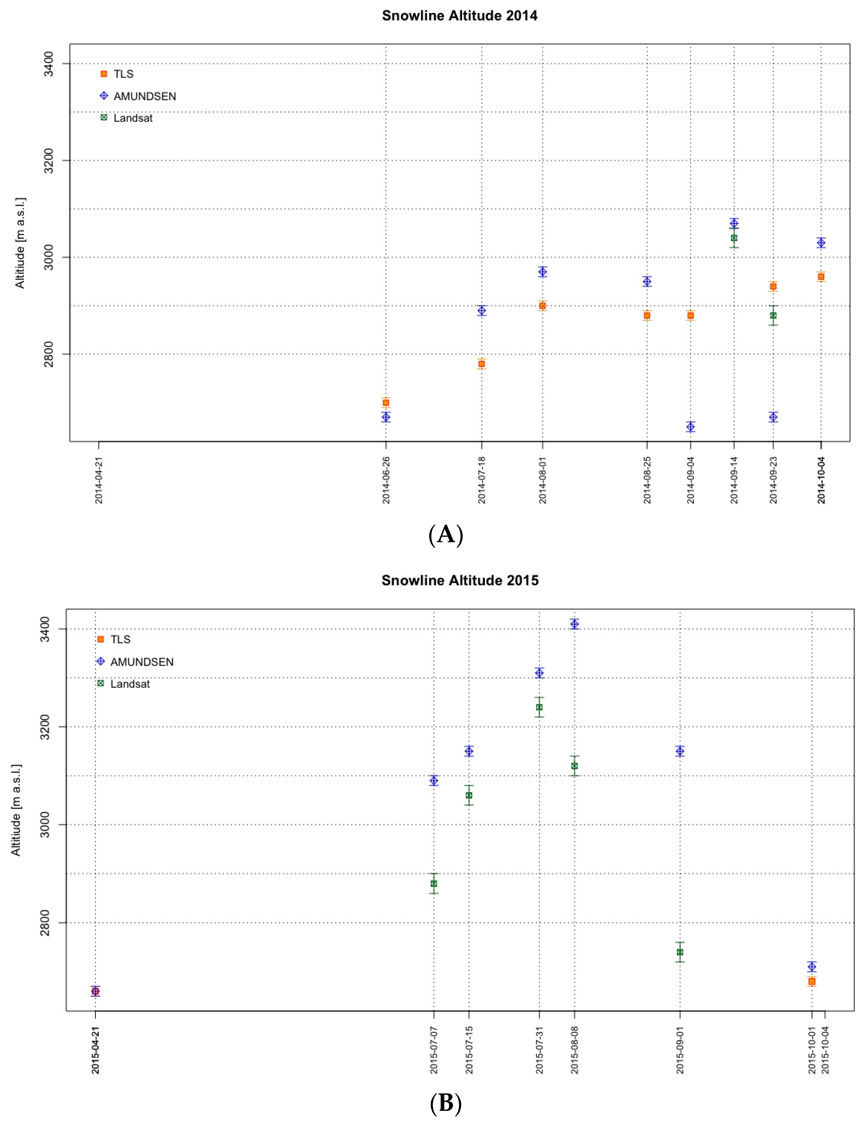
2.6. Calculation and Comparison of Snow Lines

In addition to the TLS-based method, surface classification is also performed using (i) the hydroclimatological model AMUNDSEN [67] and (ii) reflectance determination from Landsat satellite data.
With respect to (i), the AMUNDSEN model has been set up for the entire Rofental catchment to simulate the snow and ice surface energy and mass balance, as well as the resulting runoff at the catchment outlet. Model runs were performed using a spatial and temporal resolution of 50 m and 1 h, respectively. An ALS-derived DEM from the years 2006–2013 [31], resampled to 50-m resolution, glacier outlines from the year 2013 and hourly meteorological recordings of the variables air temperature, relative humidity, precipitation, global radiation, and wind speed from stations in and surrounding the catchment were entered as input data. Therefore, nine surrounding stations were used, located at elevations between 1700 and 3437 m a.s.l. (mean: 2437 m a.s.l.) and with horizontal distances to the center of HJF ranging between 6.0 and 18.7 km (mean: 12.1 km). Spatial interpolation to the model grid was performed using a combined lapse rate/inverse distance weighting approach, while for solid precipitation, an additional topographic redistribution parameterization as described in [69] was applied [70]. The simulated SWE distributions were used to derive binary snow cover maps on a daily basis (valid for 12:00 UTC) using a threshold value of 1 mm SWE.
Surface classification based on (ii) Landsat data (Landsat 7 and 8) with 30-m resolution was automatically performed for all images within the study period. The developed algorithm imports all necessary data, such as the glacier mask derived from the latest inventory and the DEM of 2006 and the respective Landsat images. The classification of snow cover is based on a ratio image using a band from the VIS (visible) and SWIR (short-wave infrared) and a respective threshold (1–1.5), resulting in a binary image. The Snow Line Altitude (SLA) is extracted by splitting the DEM into 20-m elevation bins. The classified DEM is intersected with the binary snow map and the respective glacier from the glacier mask. The SLA is assigned where the snow cover is more than 50% in the respective elevation band [71]. Although seven images were classified over the study period, only a single image coincides with the TLS scan on 23 September 2014.
For the snowline determination from TLS and AMUNDSEN, the same procedure as explained previously is used to determine the SLA. The only difference is that 10-m elevation bins were used for the intersection with the snow cover, due to the higher resolution of the TLS and AMUNDSEN data. In discussing the comparison of these methods, it is assumed that the TLS snow cover and snow line are the most accurate, because the classification is based on photos and knowledge of field works, and the TLS also has the highest spatial resolution.

3. Results and Discussion

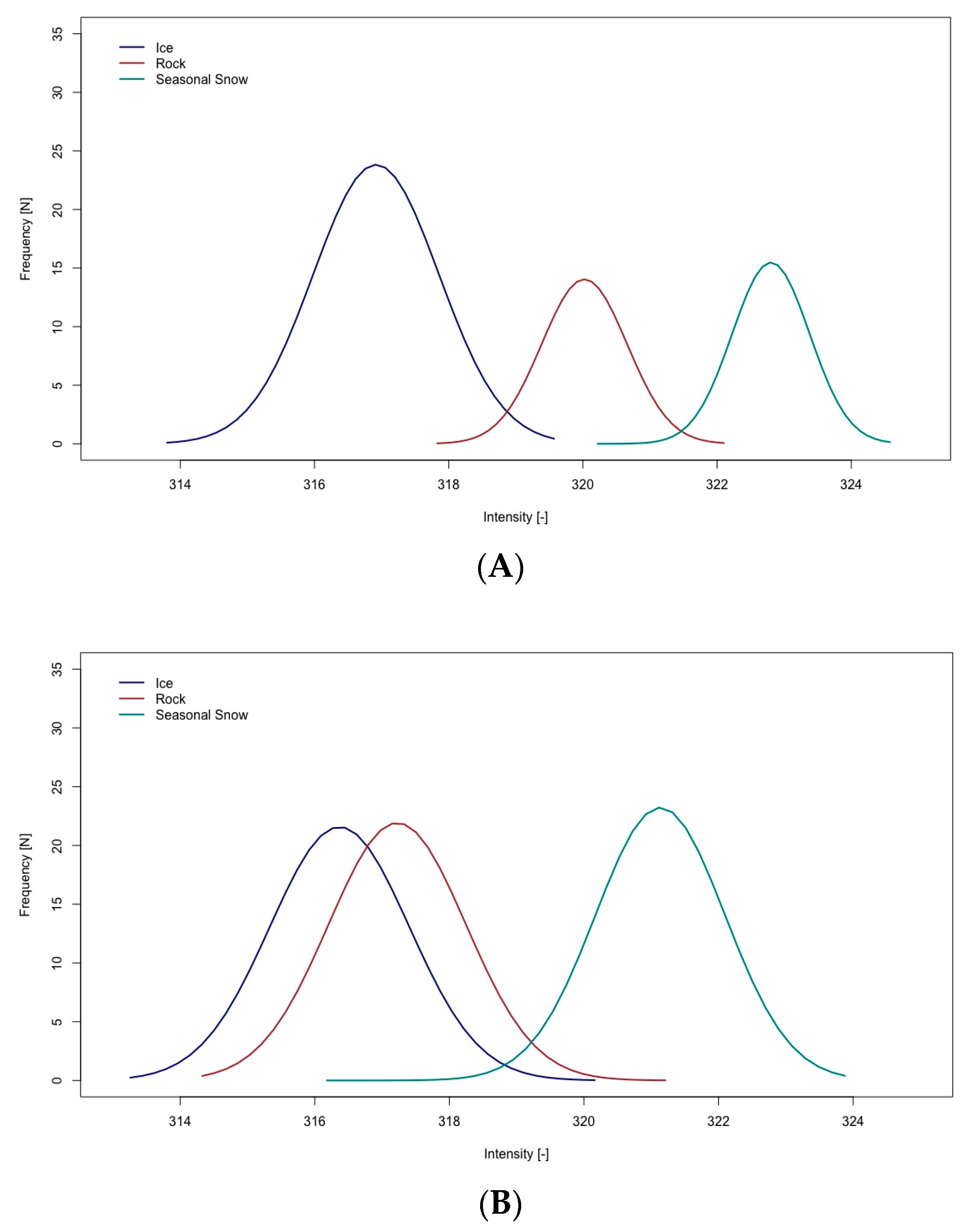
3.1. Surface Intensity and Classification

Both supervised classification methods—MLC and MDC—show similar results, but are still not as accurate as the RBC. As an example, Figure 2 presents four different raster layers of the 18 July 2014, alongside an oblique photo. At first glance, the separation of the intensity raster looks good in relation to the photograph (Figure 2A,B), but closer inspection of the intensity signals from the training areas shows that only the separation between snow and ice or snow and rocks is clearly defined, while the separation between ice and rocks is less clear due to similar reflectance properties under the scanning conditions on 18 July 2014. The temperatures were between 5 °C and 15 °C, and the humidity went up to 50%. However, under optimal scanning conditions of clear sky, low humidity (max 35%), temperatures up to 10 °C and high scan resolution, as on the 1 August 2014, the intensity signals of all three surface types are well separated (Figure 3A). It is relevant to note here that the end-of-season scans, which are perhaps of the most interest for glaciological purposes, often have less favorable atmospheric conditions; for example, on 4 September 2014, the humidity was as high as 70–80% during the scanning period (Figure 3B).
The results of the three different classification methods are compared to the ground truth data (reference data), and an error matrix is calculated. Our investigation revealed that in eight of nine scanning campaigns, RBC achieved a higher overall accuracy than MLC and MDC for glacier surface classification. For all scans, the overall accuracy of the MLC ranges between 58% and 98%; the MDC ranges between 60% and 98%; and both are outperformed by the RBC for which overall accuracy ranges from 73–100% (Table 4). Thus, while the classification from the supervised classification is generally satisfactory, the rule-based method consistently performs better, in terms of OAA, UA and PA. Misclassification in UA and PA of the MLC and MDC is primarily due to over-representation of rock in the upper part and the tongue of the glacier. Misclassification in the RBC is associated with (i) ice on the glacier tongue being classified as rock due to a thin dirt layer on the top of the glacier surface and (ii) seasonal snow being classified as ice in the upper part of the glacier due to shadow effects in the RGB photo.
Since snow has a particularly high reflectivity, the mapping and monitoring is more distinct than the other two classes. This not only appears in the error matrix, but also in the separability plots. Furthermore, the separability between the classes is highly depending on the atmospheric conditions and hence on the scanning time. The results from 1 August 2014 of the OAA, PA and UA are slightly higher for MLC and MDC than for RBC, due to very good atmospheric conditions (temperatures up to 10 °C and humidity up to 35%, clear sky and no fog). The results from 4 September 2014 have accuracies for the MLC that are low compared to the RBC and to other scan campaigns as a consequence of high humidity (up to 80%). The relatively high accuracy of the classification based on the RBC over the varying conditions of the nine scanning dates supports the first hypothesis that TLS intensity can be used successfully to determine snow cover over glacier surfaces, as the intensity of snow cover is well separated from both rock and ice.

3.2. Relationship between Intensity and Density

The correlation (Equation (4)) between intensity values and both surface and depth-averaged snow density data was used to determine if a useful relationship exists whereby TLS intensity can be taken as a proxy for either of these density parameters. The measured snow pits are shown in Figure 1, and the density, intensity and date of each snow pit are given in Table 5. The correlation between TLS intensity and snow density of the 16 snow pits is weak and insignificant. The correlation calculation of the first approach leads to r = −0.14 and the second approach to r = −0.4. These findings appear to refute the hypothesis that high intensity values correlate with low snow density. One potential reason why the correlation is low is that as the TLS campaigns took place the day after snow density measurements, the TLS intensity could be capturing a somewhat altered surface density than the field measurements; this is especially true if there were recent snow and conditions favoring snow metamorphosis or ablation during the field days. A second potential reason for the poor correlation is because the TLS measurements are partly dependent on weather conditions, which were different at each scan campaign, and therefore, the intensity value of snow varies for each scan date. Both of these factors would introduce significant noise into the relationship.

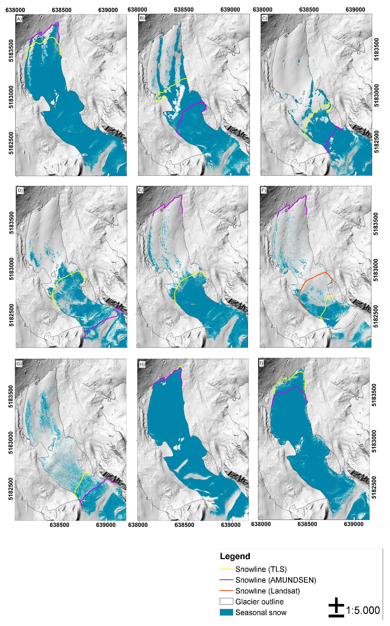
3.3. Comparison to SLA from Other Methods

As the RBC achieves surface classification accuracies >73% (mean accuracy 89%) and has the highest resolution of the three methods being compared, it is assumed to be the most reliable assessment of the true snowline. From the example on the 18 July 2014 (Figure 2), it can be seen that the snow distribution is not simply related to elevation on the glacier surface and instead forms a more complex pattern related to longitudinal ridges on the glacier tongue and shadowing and local curvature in the upper glacier. Therefore, it is evident that the method of determining SLA applied here represents a gross simplification of the true snow distribution over the glacier surface. Nevertheless, SLA defined in this way remains a useful metric for methodological intercomparison and is also widely used as a proxy for the glacier mass balance conditions throughout the ablation season.
Progressive changes in SLA can be seen in Figure 4 and Figure 5. In 2014, the TLS snowline shows a progressive increase over the summer season from 2700 m up to 2960 m. The TLS snowline rose only slowly in summer 2014, due to cold and rainy/snowy weather conditions. From June–August, the change in snowline altitude is faster than from August–mid-September. In the latter period, the weather conditions are humid and cold, and therefore, the snowline is steady at about 2880 m. At the end of the summer season, it moves up ~100 m (2960 m). The AMUNDSEN SLA tracks the TLS SLA quite well, though with a slight positive bias, through the 2014 ablation season up until the end of August. However, AMUNDSEN produces some large excursions from the TLS SLA in September 2014, predicting much lower SLA than determined by the TLS surface classification.
In 2015, only two TLS scan campaigns were carried out, and therefore, observations of the behavior of the seasonal snowline evolution are not possible. In 2015, the end of season scan campaign was on 1 October, by which the whole glacier was already covered by snow, and therefore, the snowline was very low.
Coincident data for all three methods are only available on 22/23 September 2014, when the Landsat and AMUNDSEN snowlines underestimate the TLS snowline by 60 and 270 m, respectively. Table 6 and Figure 4 and Figure 5 compare all available snowline data, in terms of SLA and snow-covered area, for the dates of TLS-, AMUNDSEN- and Landsat-derived SLA. Comparing the TLS and AMUNDSEN SLAs, the elevation difference between methods exceeds 200 m for only three cases (see Table 6) (up to 300 m); in most cases, both snowlines are close to each other. At the start and end of the season, the AMUNDSEN model captures the same behavior of the snowline as the TLS does. The AMUNDSEN SLA coincides well with the TLS SLA at the beginning of both the 2014 and 2015 ablation seasons and again at the end of the 2015 ablation season. At the end of the 2014 ablation, AMUNDSEN slightly overestimates the TLS SLA, but overall, the comparison at the seasonal timescale suggests that the AMUNDSEN simulations can produce realistic snowline altitudes at the seasonal scale (Figure 6). Furthermore, the Accumulation Area Ratio (AAR) for each date and snowline altitude is given in Table 6.
The Landsat and AMUNDSEN snowlines are compared twice in 2014: firstly, in mid-September, where the Landsat SLA is only 30 m below the AMUNDSEN SLA, and at end of September, when the Landsat SLA is 200 m above the AMUNDSEN SLA (see Table 6). However, five Landsat images are available in 2015, and for these dates, the Landsat SLA is consistently below the AMUNDSEN SLA, corroborating the positive bias in the AMUNDSEN SLA suggested by comparison to the TLS SLA during 2014. For late-season Landsat imagery, part of the discrepancy between the AMUNDSEN and satellite-derived SLA can be attributed to the low Sun angle, which causes substantial shadowing in the Landsat image, due to north-facing slopes. Another reason is the stepped form of the glacier. There are two plateaus: one in the upper part and one in the middle part of HJF. Furthermore, the two plateaus have an impact on the quality of the intensity data (see the data gaps in Figure 2 and Figure 5). The plateau on the upper part of the glacier could not be scanned from the highest scan positions on the opposite slope. At the second plateau in the middle of the glacier, the angle of incidence is very low, and therefore, no signal returned to the laser scanner. As a result of both plateaus and ridges in the line of sight, some areas could not be scanned. The maximum percentage of the glacier from all three scan positions is 75.9% and the minimum only 61.3%. The average area of the glacier is 70.8%.
Pfeifer et al. [37] (p. 1050) suggest that laser scanning should be “[…] considered a 4D measurement process”, because not only x-, y- and z-coordinates are collected, but also the intensity of each point. TLS data have bene shown to be a valuable tool in glaciological and snow process measurements. The work in [34] calculated the mass balance of five small glaciers based on TLS measurements and compared their results with glaciological mass balances. In contrast to the study by [34], we demonstrate the potential for identifying surface material properties using the signal intensity of a terrestrial laser scan for a glaciological application. The intensity-based MLC and MDC method applied here is satisfying for classifying snow, because the intensity separation between snow and ice/rock is obvious; however, RBC produces consistently more accurate surface classification. In high mountain environments, the maximum scanning range is achieved when the temperatures are low and the atmosphere is dry [24,57,72], and we found these to also be optimal conditions for signal separation for snow ice and rock. Despite the overall good performance of the best classification method, reflectance irregularities can still cause inaccuracies, and not only intensity data, but also additional data from the TLS are needed as the input dataset to resolve these issues. The reflectance changes with, for example, dirt on the surface, moisture and grain size. If exposed rock is wet, the intensity is lower than if it were dry rock, and RGB imagery from the TLS can help resolve these surface conditions. If a fine layer of dirt is on the ice surface, the intensity increases, but as this surface still has a low roughness value, the RBC still correctly identifies the pixel as ice, whereas it would be misclassified in the MLC or MDC.
Both the range and the angle of incidence affect the intensity strongly. Studies show that the incidence angle of a laser beam changes along with the distance. Large angles of incidence and also low reflectivity of the surface decrease the intensity of the signal return [36,73,74,75]. Thus, it is important to have a good vantage point overlooking the surface of interest and also a scanning vantage point as close to the surface as possible. This is problematic for the case of mountain glaciers, which are large targets, spanning several kilometers in length and several hundred meters in elevation. Finding suitable locations for scanning that can overlook the upper reaches of glaciers originating in the high mountains is challenging, and the occurrence of gently inclined accumulation bowls as in the upper HJF is not uncommon, but causes problems for oblique TLS view angles. Thus, the suitability and success of applying the method presented here on a given glacier will depend partly on its topographic surroundings and surface geometry. Furthermore, a post-processed atmospheric correction can be useful, when comparing the intensity of different scan campaigns. Krooks et al. [54], Pfeifer et al. [21] Pfeifer et al. [37], Höfle and Pfeifer [36] and Kaasalainen et al. [73] have good approaches to correct laser scanning intensity values.
The data have a high resolution with 1 m2 grid cells. In seven of nine datasets, the number of average points per cell is eight, and in the two other sets, it is 15 (due to higher frame resolution). Therefore, more than one point measurement is used to define one intensity grid cell value. Within this grid cell, more than one surface class can be present, which leads to small-scale variability.
Using a TLS for capturing snow distribution on a glacier and its surroundings is a powerful method and outperforms SLA assessments from optical satellite data. The Landsat data used in this study have a resolution of 30 m; therefore, a small-scale distribution and glacial facies are not clearly detectable due to low radiometric resolution (eight bit). For example, if the glacier tongue is covered by a dust layer, the glacier extents are difficult to separate from the rocks in the neighborhood [76]. Additionally, compared to optical images, e.g., Landsat data, laser scanning data have no shadow effects. This is especially an advantage in high mountain environments, because due to the mountains, large areas can be covered in shadow [39].
The difference between the TLS snowline and the Landsat snowline from the 22/23 September 2014 results/emerges, on the one hand, from the stepped-shape of the glacier and, on the other, from the glacier’s exposition. The north exposure leads to huge shadow areas at this time of the year, and therefore, an automatic classification is difficult. The Landsat snowline is about 60 m lower than the TLS one (see Table 6).
The snowline simulated with the AMUNDSEN model partly shows very large deviations from the TLS or Landsat-derived values. Further investigation showed that the AMUNDSEN snowlines are very sensitive to the SWE threshold value for some of the investigated days. For example, on 23 September 2014, changing the threshold value from 1 to 10 mm results in an upward shift of the resulting snowline of 480 m, as a very thin snow layer is present on the lower parts of the glacier on this day likely due to an earlier precipitation event misclassified as snowfall by the model. The selected threshold value of 1 mm as already used in other studies in the same area (e.g., [70]) resulted in average deviations of 21 m for the TLS-derived snowline, as compared to 114 m when using a threshold value of 10 mm.
It is not uncommon that the number of glaciological mass balance measurements in the upper glacier are sparse and sometimes not well distributed, due to access limitations (e.g., [14,15,34]). Therefore, resolving the true snowline from these point measurements can lead to significant inaccuracies. The application of high spatial resolution, accurate snowlines to end of season glacier surfaces offers the possibility to improve the accuracy of annual glacier-wide mass balance assessments [17,34].

4. Conclusions and Outlook

This research investigated the possibilities of a surface classification based on terrestrial laser scanning intensity data. The signal intensity of snow proved to be well separable from other glacier surface types, but the ground control samples and error matrices reveal low separability between ice and rock. Three different classification methods were compared: two supervised classifications (MLC and MDC) and one RBC. The main result of the classification analyses shows that in the case of generating the classification by just using the intensity data (supervised classification), the results are highly dependent on the atmospheric conditions. If the conditions are good (low temperatures, dry air, low moist content), a classification based on TLS intensity data alone is acceptable. Otherwise, a rule-based classification, based on intensity, surface roughness and a photo taken by the scanner, is more precise. A rule-based classification improves the classification results in different ways. For example, although rock has a similar signal intensity as ice and is therefore subject to being misclassified as ice, it will be classified correctly, when taking the RGB data into account, as its RGB value is clearly darker than that of ice. This makes the RBC more reliable in the variable atmospheric conditions of the mountain environment.
TLS VZ-6000 provides good data for classification, especially if only the snow distribution is identified. Therefore, it has high potential for applications in snow modelling and hydrological studies. Further studies should consider an atmospheric correction, even though the VZ-6000 laser scanner calibrates the atmosphere effects automatically.
Valuable future work on generating high resolution snow line altitudes over glaciers could include: (i) a comparison between Sentinel-2A and new TLS data, since Sentinel-2A data have a resolution of 10 m and are also freely available; (ii) the Landsat (7/8) data should be resampled using the panchromatic band to get a snow classification raster layer with a 15-m resolution [76]. Additionally, the impact of using high resolution snow line altitude information on calculated glacier mass balance would provide a quantified assessment of the impact of improving the snowline resolution.

Acknowledgments

This work was part of the “hiSnow—High resolution monitoring and modelling under climate change conditions” project, which was funded by the Autonomous Province of Bolzano—Alto Adige. Glaciological field data used in this study were collected by Rainer Prinz, Hannah Prantl, Franz Grüsser and Lindsey Nicholson.

Author Contributions

R.S. conceived of the study. H.P. collected and analyzed the TLS data and prepared the figures. F.H. performed the AMUNDSEN model runs. P.R. did the Landsat satellite classification. H.P., L.N. and I.F.J. led the preparation of the manuscript, to which all authors contributed.

Conflicts of Interest

The authors declare no conflict of interest. The founding sponsors had no role in the design of the study; in the collection, analyses or interpretation of data; in the writing of the manuscript; nor in the decision to publish the results.

References

  1. Zemp, M.; Hoelzle, M.; Haeberli, W. Six Decades of Glacier Mass-Balance Observations: A Review of the Worldwide Monitoring Network. Ann. Glaciol. 2009, 50, 101–111. [Google Scholar] [CrossRef] [Green Version]
  2. Zemp, M.; Thibert, E.; Huss, M.; Stumm, D.; Rolstad Denby, C.; Nuth, C.; Nussbaumer, S.U.; Moholdt, G.; Mercer, A.; Mayer, C.; et al. Reanalysing Glacier Mass Balance Measurement Series. Cryosphere 2013, 7, 1227–1245. [Google Scholar] [CrossRef] [Green Version]
  3. Kaser, G.; Cogley, J.G.; Dyurgerov, M.B.; Meier, M.F.; Ohmura, A. Mass Balance of Glaciers and Ice Caps: Consensus Estimates for 1961–2004. Geophys. Res. Lett. 2006, 33, 1–5. [Google Scholar] [CrossRef]
  4. Marzeion, B.; Jarosch, A.H.; Hofer, M. Past and Future Sea-Level Change from the Surface Mass Balance of Glaciers. Cryosphere 2012, 6, 1295–1322. [Google Scholar] [CrossRef] [Green Version]
  5. Gardner, A.S.; Moholdt, G.; Cogley, J.G.; Wouters, B.; Arendt, A.A.; Wahr, J.; Berthier, E.; Hock, R.; Pfeffer, W.T.; Kaser, G.; et al. Reconciled Estimate of Glacier Contributions to Sea Level Rise: 2003 to 2009. Science 2013, 340, 852–857. [Google Scholar] [CrossRef] [Green Version]
  6. Vaughan, D.G.; Comiso, J.C.; Allison, I.; Carrasco, J.; Kaser, G.; Kwok, R.; Mote, P.; Murray, T.; Paul, R.; Ren, J.; et al. Observations: Cryosphere. In Climate Change 2013: The Physical Science Basis; Contribution of Working Group I to the Fifth Assessment Report of the Intergovernmental Panel on Climate Change; Stocker, T.F., Qin, D., Plattner, G.-K., Tignor, M., Allen, S.K., Boschung, J., Nauels, A., Xia, Y., Bex, V., Midgley, P.M., Eds.; Cambridge University Press: Cambridge, UK; New York, NY, USA, 2014. [Google Scholar]
  7. Kaser, G.; Grosshauser, M.; Marzeion, B. Contribution Potential of Glaciers to Water Availability in Different Climate Regimes. Proc. Natl. Acad. Sci. USA 2010, 107, 20223–20227. [Google Scholar] [CrossRef] [PubMed]
  8. Marzeion, B.; Cogley, J.G.; Richter, K.; Parkes, D. Attribution of Global Glacier Mass Loss to Anthropogenic and Natural Causes. Science 2014, 919–921. [Google Scholar] [CrossRef] [PubMed]
  9. Slangen, A.B.A.; Church, J.A.; Agosta, C.; Fettweis, X.; Marzeion, B.; Richter, K. Anthropogenic Forcing Dominates Global Mean Sea-Level Rise since 1970. Nat. Clim. Chang. 2016, 11–16. [Google Scholar] [CrossRef]
  10. Radić, V.; Hock, R. Modeling Future Glacier Mass Balance and Volume Changes Using ERA-40 Reanalysis and Climate Models: A Sensitivity Study at Storglaciaren, Sweden. J. Geophys. Res. 2006, 111. [Google Scholar] [CrossRef]
  11. Radić, V.; Bliss, A.; Beedlow, A.C.; Hock, R.; Miles, E.; Cogley, J.G. Regional and Global Projections of Twenty-First Century Glacier Mass Changes in Response to Climate Scenarios from Global Climate Models. Clim. Dyn. 2013, 42, 37–58. [Google Scholar] [CrossRef]
  12. Huss, M.; Hock, R. A New Model for Global Glacier Change and Sea-Level Rise. Front. Earth Sci. 2015, 3, 1–22. [Google Scholar] [CrossRef]
  13. Mengel, M.; Levermann, A.; Frieler, K.; Robinson, A.; Marzeion, B.; Winkelmann, R. Future Sea Level Rise Constrained by Observations and Long-Term Commitment. Proc. Natl. Acad. Sci. USA 2016, 113, 2597–2602. [Google Scholar] [CrossRef]
  14. Galos, S.P.; Klug, C.; Maussion, F.; Covi, F.; Nicholson, L.; Rieg, L.; Gurgiser, W.; Mölg, T.; Kaser, G. Reanalysis of a Ten Year Record (2004–2013) of Seasonal Mass Balances at Langenferner/Vedretta Lunga, Ortler-Alps, Italy. Cryosphere 2017, 11, 1417–1439. [Google Scholar] [CrossRef]
  15. Klug., C.; Bollmann, E.; Prinz, R.; Galso, S.P.; Rieg, L.; Kaser, G.; Sailer, R. A detailed comparison of 10 years of annual glacier mass balance obtained by geodetic and glaciological methods at Hintereisferner, Ötztal Alps, Austria. Cryosphere 2017. in preparation. [Google Scholar]
  16. Pelto, M.; Kavanaugh, J.; McNeil, C. Juneau Icefield Mass Balance Program 1964–2011. Earth Syst. Sci. Data 2013, 5, 319–330. [Google Scholar] [CrossRef]
  17. Mernild, S.; Pelto, M.; Malmros, J.; Yde, J.; Knudsen, N.; Hanna, E. Identification of Snow Ablation Rate, ELA, AAR and Net Mass Balance using Transient Snowline Variations on two Arctic Glaciers. J. Glaciol. 2013, 59, 649–659. [Google Scholar] [CrossRef]
  18. Mölg, N.; Ceballos, J.L.; Huggel, C.; Micheletti, N.; Rabatel, A.; Zemp, M. Ten years of montly Mass Balance of Conejeras Glacier, Colombia, and their Evaluation using Different Interpolation Methods. Geogr. Ann. Ser. A Phys. Geogr. 2017, 1–22. [Google Scholar] [CrossRef]
  19. Rabatel, A.; Dedieu, J.-P.; Vincent, C. Using Remote-Sensing Data to Determine Equilibrium-line Altitude and Mass-Balance Time Series: Validation on three French Glaciers, 1994–2002. J. Glaciol. 2005, 51, 539–546. [Google Scholar] [CrossRef]
  20. Mizukami, N.; Perica, S. Spatiotemporal Characteristics of Snowpack Density in the Mountainous Regions of the Western United States. J. Hydrometeorol. 2008, 9, 1416–1426. [Google Scholar] [CrossRef]
  21. Pfeifer, N.; Briese, C. Geometrical Aspects of Airborne Laser Scanning and Terrestrial Laser Scanning; Rönnholm, P., Hyyppä, H., Hyyppä, J., Eds.; International Archives of Photogrammetry and Remote Sensing: Espoo, Finland, 2007. [Google Scholar]
  22. Geist, T.; Lutz, E.; Stötter, J. Airborne laser scanning technology and its potentials for applications in glaciology. In 3-D Reconstruction from Airborne Laserscanner and INSAR Data; Maas, H.G., Vosselman, G., Streilein, A., Eds.; ISPRS Workshop: Dresden, Germany, 2003. [Google Scholar]
  23. Sailer, R.; Bollmann, E.; Hoinkes, S.; Rieg, L.; Spross, M.; Stötter, J. Quantification of Geomorphodynamics in Glaciated and Recently Deglaciated Terrain based on Airborne Laser Scanning Data. Geogr. Ann. Ser. A Phys. Geogr. 2012, 94, 17–32. [Google Scholar] [CrossRef]
  24. López-Moreno, J.I.; Revuelto, J.; Alonso-Gonzáles, E. Using very long-range Terrestrial Laser Scanning to Analyze the Temporal Consistency of the Snowpack Distribution in a High Mountain Environment. J. Mt. Sci. 2017, 14, 823–842. [Google Scholar] [CrossRef]
  25. Blasone, G.; Cavalli, M.; Marchi, L.; Cazorzi, F. Monitoring Sediment Source Areas in a Debris-Flow Catchment using Terrestrial Laser Scanning. Catena 2004, 123, 23–36. [Google Scholar] [CrossRef]
  26. Gabbud, C.; Micheletti, N.; Lane, S.N. Instruments and methods. LiDAR measurements of surface melt for a temperate alpine glacier at the seasonal ad hourly scales. J. Glaciol. 2015, 61, 963–974. [Google Scholar] [CrossRef]
  27. Jörg, P.; Fromm, R.; Sailer, R.; Schaffhauser, A. Measuring Snow Depth with a Terrestrial Laser Ranging System. In Proceedings of the 2006 International Snow Science Workshop (ISSW), Telluride, CO, USA, 1–6 October 2006; pp. 452–460. [Google Scholar]
  28. Schaffhauser, A.; Fromm, R.; Joerg, P.; Luzi, G.; Noferini, L.; Sailer, R. Remote Sensing Based Retrieval of Snow Cover Properties. Cold Reg. Sci. Technol. 2008, 54, 164–175. [Google Scholar] [CrossRef]
  29. Sailer, R.; Fellin, W.; Fromm, R.; Jörg, P.; Rammer, L.; Sampl, P.; Schaffhauser, A. Snow Avalanche Mass-Balance Calculation and Simulation-Model Verification. Ann. Glaciol. 2008, 48, 183–192. [Google Scholar] [CrossRef]
  30. Prokop, A. Assessing the Applicability of Terrestrial Laser Scanning for Spatial Snow Depth Measurements. Cold Reg. Sci. Technol. 2008, 54, 155–163. [Google Scholar] [CrossRef]
  31. Schwalbe, E.; Maas, H.G.; Dietrich, R.; Ewert, H. Glacier Velocity Determination from Multi Temporal Terrestrial Long Range Laser Scanner Point Clouds. In Proceedings of the ISPRS Congress Beijing 2008, Beijing, China, 3–11 July 2008. [Google Scholar]
  32. Bauer, A.; Paar, G.; Kaufmann, V. Terrestrial Scanning for Rock Glacier Monitoring. In Proceedings of the 8th International Conference on Permafrost, Zurich, Switzerland, 21–25 July 2003. [Google Scholar]
  33. Kellerer-Pirklbauer, A.; Bauer, A.; Proske, H. Terrestrial Laser Scanning for Glacier Monitoring: Glaciation Changes of the Gössnitzkees Glacier (Schober Group, Austria) between 2000 and 2004. In Proceedings of the 3rd Symposium of the Hohe Tauern National Park for Research in Protected Areas, Castle of Kaprun, Austria, 15–17 September 2005; Phillips, M., Springman, S.M., Arenson, L.U., Eds.; pp. 97–106. [Google Scholar]
  34. Fischer, M.; Huss, M.; Kummert, M.; Hoelzle, M. Application and Validation of long-range Terrestrial Laser Scanning to Monitor the Mass Balance of very small Glaciers in the Swiss Alps. Cryosphere 2016, 10, 1279–1295. [Google Scholar] [CrossRef]
  35. Dumont, M.; Sirguey, P.; Arnaud, Y.; Six, D. Monitoring Spatial and Temporal Variations of Surface Albedo on Saint Sorlin Glacier (French Alps) using Terrestrial Photography. Cryosphere 2011, 5, 759–771. [Google Scholar] [CrossRef] [Green Version]
  36. Höfle, B.; Pfeifer, N. Correction of laser scanning intensity data: Data and model-driven approaches. J. Photogramm. Remote Sens. 2007, 62, 415–433. [Google Scholar] [CrossRef]
  37. Pfeifer, N.; Höfle, B.; Briese, C.; Rutzinger, M.; Haring, A. Analysis of the Backscattered Energy in Terrestrial Laser Scanning Data. In Proceedings of the ISPRS Congress Beijing 2008, Beijing, China, 3–11 July 2008; pp. 1045–1051. [Google Scholar]
  38. Jörg, P.C.; Weyermann, J.; Morsdorf, F.; Zemp, M.; Schaepman, M.E. Computation of a Distributed Glacier Surface Albedo using Airborne Laser Scanning Intensity Data and in-situ Spectro-Radiometric Measurements. Remote Sens. Environ. 2015, 160, 31–42. [Google Scholar] [CrossRef]
  39. Fritzmann, P.; Höfle, B.; Vetter, M.; Sailer, R.; Stötter, J.; Bollmann, E. Surface classification based on multi-temporal airborne LiDAR intensity data in high mountain environments. A case study from Hintereisferner, Austria. Z. Geomorphol. 2011, 55, 105–126. [Google Scholar] [CrossRef]
  40. Tiroler Landesregierung. Available online: https://www.tirol.gv.at/data/datenkatalog/geographie -und-planung/digitales-gelaendemodell-tirol/ (accessed on 20 April 2017).
  41. Corine Land Cover 2006 Raster Data. The European Topic Centre on Land Use and Spatial Information. Available online: http://www.eea.europa.eu/data-and-maps/data/corine-land-cover-2006-clc2006 -100-m-version-12–2009#tab-gis-data (accessed on 15 March 2014).
  42. Fliri, F. Das Klima der Alpen im Raume von Tirol: Monographie zur Landeskunde Tirols, 1st ed.; Wagner: Innsbruck, Austria; München, Germany, 1975. [Google Scholar]
  43. Kuhn, M.; Batlogg, N. Glacier Runoff in Alpine Headwaters in a Changing Climate. Hydrol. Water Resour. Ecol. Headwaters 1998, 248, 79–88. [Google Scholar]
  44. Kuhn, M.; Nickus, U.; Pellet, F. Die Niederschlagsverhältnisse im inneren Ötztal. In 17. Internationale Tagung für Alpine Meteorologie, Berchtesgaden, Germany, 21–25 September 1982; Selbstverlag des Deutschen Wetterdienstes: Offenbach, Germany, 1982. [Google Scholar]
  45. Kuhn, M.; Dreiseitl, E.; Emprechtinger, M. Temperatur und Niederschlag an der Wetterstation Obergurgl, 1953–2011. In Klima, Wetter, Gletscher im Wandel; Koch, E.-M., Erschbamer, B., Eds.; Innsbruck University Press (IUP): Innsbruck, Austria, 2013; Volume 9, pp. 11–31. [Google Scholar]
  46. Kuhn, M.; Abermann, J.; Olefs, M.; Fischer, A.; Lambrecht, A. Gletscher im Klimawandel: Aktuelle Monitoring Programme und Forschungen zur Auswirkung auf den Gebietsabfluss im Ötztal. In Mitteilungsblatt des hydrographischen Dienstes Österreich, 1st ed.; Austrian Ministry for Agriculture, Forestry, Environment and Water Management (BMLFUW): Vienna, Austria, 2009; Volume 86, pp. 31–47. [Google Scholar]
  47. Juen, I.; Kaser, G. Climate Data Vent, Ötztal Alps, 2012–2016; Dataset #876595; Pangaea: Bremen, Germany, 2017; Available online: https://doi.pangaea.de/10.1594/PANGAEA.876595 (accessed on 28 June 2017).
  48. Juen, I.; Kaser, G.; Niedertscheider, K. Monthly Precipitation at Gauge Station Rofenberg 1952–01 to 2016–12; Dataset #876528; Pangaea: Bremen, Germany, 2017; Available online: https://doi.pangaea.de/10.1594/PANGAEA.876528 (accessed on 28 June 2017).
  49. Riegl. 3-D Terrestrial Laser Scanner RIEGL VZ-4000/RIEGL VZ-6000. General Description and Data Interfaces, 3rd ed.; Riegl: Horn, Austria, 2014. [Google Scholar]
  50. Conrad, O.; Bechtel, B.; Bock, M.; Dietrich, H.; Fischer, E.; Gerlitz, L.; Wehberg, J.; Wichmann, V.; Böhner, J. System for Automated Geoscientific Analyses (SAGA) v. 2.1.4. Geosci. Model Dev. 2015, 8, 1991–2007. [Google Scholar] [CrossRef]
  51. Yunfei, B.; Guoping, L.; Chunxiang, C.; Xiaowen, L.; Hao, Z.; Qisheng, H.; Linyan, B.; Chaoyi, C. Classification of LiDAR Point Cloud and Generation of DTM from LiDAR Height and Intensity Data in Forested Area. The International Archives of the Photogrammetry, Remote Sensing and Spatial Information Sciences. In Proceedings of the ISPRS Congress Beijing 2008, Beijing, China, 3–11 July 2008. [Google Scholar]
  52. El-Ashmawy, N.; Shaker, A. Raster vs. Point Cloud LiDAR Data Classification. In Proceedings of the ISPRS Technical Commission VII Symposium, Istanbul, Turkey, 29 September–2 October 2014. [Google Scholar]
  53. Wagner, W.; Ullrich, A.; Ducic, V.; Melzer, T.; Studnicka, N. Gaussian Decomposition and Calibration of a Novel Small-Footprint Full-Waveform digitising Airborne Laser Scanner. J. Photogramm. Remote Sens. 2006, 60, 100–112. [Google Scholar] [CrossRef]
  54. Krooks, A.; Kaasalainen, S.; Hakala, T.; Nevalainen, O. Correction of Intensity Incidence Angle Effect in Terrestrial Laser Scanning. In Proceedings of the ISPRS Workshop Laser Scanning 2013, Antalya, Turkey, 11–13 November 2013. [Google Scholar]
  55. Arnold, N.S.; Rees, W.G.; Devereux, B.J.; Amable, G.S. Evaluating the Potential of High-Resolution Airborne LiDAR Data in Glaciology. Int. J. Remote Sens. 2006, 27, 1233–1251. [Google Scholar] [CrossRef]
  56. Geist, T. Application of Airborne Laser Scanner Technology in Glacier Research. Doctor Dissertation, University of Innsbruck, Innsbruck, Austria, 2005. [Google Scholar]
  57. Baltsavias, E.P. A Comparison between Photogrammetry and Laser Scanning. J. Photogramm. Remote Sens. 1999, 54, 83–94. [Google Scholar] [CrossRef]
  58. Baltsavias, E.P. Airborne Laser Scanning: Basic Relations and Formulas. J. Photogramm. Remote Sens. 1999, 54, 199–214. [Google Scholar] [CrossRef]
  59. Wagner, W.; Hyyppä, J.; Ullrich, A.; Lehner, H.; Briese, C.; Kaasalainen, S. Radiometric Calibration of Full-Waveform Small-Footprint Airborne Laser Scanners. The International Archives of the Photogrammetry, Remote Sensing and Spatial Information Sciences. In Proceedings of the ISPRS Congress Beijing 2008, Beijing, China, 3–11 July 2008. [Google Scholar]
  60. Antilla, K.; Hakala, T.; Kaasalainen, S.; Kaartinen, H.; Nevalainen, O.; Krooks, A.; Kukko, A.; Jaakkola, A. Calibrating Laser Scanner Data from Snow Surfaces: Correction of Intensity Effects. Cold Reg. Sci. Technol. 2016, 121, 52–59. [Google Scholar] [CrossRef]
  61. Pfeifer, N.; Briese, C. Laser Scanning—Principles and Applications. In Proceedings of the 3rd International Exhibition and Scientific Congress GeoSiberia 2007, Novosibirsk, Russia, 25–27 April 2007. [Google Scholar]
  62. Albretz, J.; Wiggenhagen, M. Taschenbuch zur Photogrammetrie und Fernerkundung. In Guide for Photogrammetry and Remote Sensing, 5th ed.; Wichmann: Heidelberg, Germany, 2009. [Google Scholar]
  63. Richard, J.A.; Jia, W. Remote Sensing Digital Image Analysis: An Introduction, 4th ed.; Springer-Verlag: Berlin, Germany, 2006. [Google Scholar]
  64. ERDAS. ERDAS Field Guide, 5th ed.; ERDAS: Atrlanta, GA, USA, 1999. [Google Scholar]
  65. Lillesand, T.M.; Kiefer, R.W.; Chipman, J.W. Remote Sensing and Image Interpretation, 7th ed.; Wiley: Hoboken, NJ, USA, 2008. [Google Scholar]
  66. Höfle, B.; Geist, T.; Rutzinger, M.; Pfeifer, N. Glacier Surface Segmentation Using Airborne Laser Scanning Point Cloud and Intensity Data; Rönnholm, P., Hyyppä, H., Hyyppä, J., Eds.; International Archives of Photogrammetry and Remote Sensing: Espoo, Finland, 2007. [Google Scholar]
  67. Congalton, R.G.; Green, K. Assessing the Accuracy of Remotely Sensed Data: Principles and Practices, 2nd ed.; Tylor & Francis Group: Boca Raton, FL, USA, 2009. [Google Scholar]
  68. Zimmermann-Janschitz, S. Statistik in der Geographie. Eine Exkursion Durch Die Deskriptive Statistik, 1st ed.; Springer Spektrum: Berlin, Germany, 2014. [Google Scholar]
  69. Strasser, U. Die Modellierung der Gebirgsschneedecke im Nationalpark Berchtesgaden; Nationalparkverwalt. Berchtesgaden: Berchtesgaden, Germany, 2008. [Google Scholar]
  70. Hanzer, F.; Helfricht, K.; Marke, T.; Strasser, U. Multilevel spatiotemporal validation of snow/ice mass balance and runoff modeling in glacierized catchments. Cryosphere 2016, 10, 1859–1881. [Google Scholar] [CrossRef]
  71. Rastner, P.; Nicholson, L.; Sailer, R.; Notarnicola, C.; Prinz, R. Mapping the Snow Line Altitude for Large Glacier Samples from Multitemporal Landsat Imagery. In Proceedings of the 2015 8th International Workshop on the Analysis of Multitemporal Remote Sensing Images (Multi-Temp), Annecy, France, 22–24 July 2015. [Google Scholar]
  72. Deems, J.S.; Painter, T.H.; Finnegan, D.C. LiDAR Measurements of Snow Depth: A Review. J. Glaciol. 2013, 59, 467–479. [Google Scholar] [CrossRef]
  73. Kaasalainen, S.; Hyyppä, H.; Kukko, A.; Litkey, P.; Ahokas, E.; Hyyppä, J.; Lehner, H.; Jaakkola, A.; Suomalainen, J.; Akujärvi, A.; et al. Radiometric Calibration of LiDAR Intensity with Commercially Available Reference Targets. IEEE Trans. Geosci. Remote Sens. 2009, 2, 588–598. [Google Scholar] [CrossRef]
  74. Kaasalainen, S.; Kaartinen, H; Kukko, A. Snow Cover Change Detection with Laser Scanning Range and Brightness Measurements. EARSeL Eproc. 2008, 7, 133–141. [Google Scholar]
  75. Hollaus, M.; Mandlburger, G.; Pfeifer, N.; Mücke, W. Land Cover Dependant Derivation of Digital Surface Models from Airborne Laser Scanning Data; Paparoditis, N., Pierrot-Deseilligny, M., Mallet, C., Tournaire, O., Eds.; IAPRS: Saint-Mandé, France, 2010. [Google Scholar]
  76. Paul, F.; Winsvold, S.H.; Kääb, A.; Nagler, T.; Schwaizer, G. Glacier Remote Sensing Using Sentinel-2. Part II: Mapping Glacier Extents and Surface Facies, and Comparison to Landsat 8. Remote Sens. 2016, 8, 1–15. [Google Scholar] [CrossRef]
Figure 1. Overview map showing the surface divisions of the ice body that is called Hochjochferner. The part of Hochjochferner studied here is the mass balance area. Locations of Terrestrial Laser Scanner (TLS) scan positions, reflectors for georeferencing TLS scans, ablation stakes and snow pits are all shown. The map coordinate system is displayed as WGS1984 UTM Zone 32N, and the background of the map is a hillshade based on Airborne Laser Scanning (ALS) data, overlaid with an ESRI Bing Map.
Geosciences 07 00060 g001
Figure 2. The (A) intensity (signal strength) raster layer, (B) photograph of the glacier (looking upglacier, in an approximately SSW direction) taken on 17 July 2017 (with the location of the snow pit), the (C) Rule-Based Classified (RBC), the (D) Maximum-Likelihood supervised Classified (MLC) and the (E) minimum distance supervised classified raster layer of 18 July 2014.
Geosciences 07 00060 g002
Figure 3. Intensity distribution per surface class from (A) 1 August 2014 and (B) 4 September 2014. The good separability on 1 August is a result of optimal scan conditions, and the low separability of 4 September 2014 is due to weather conditions.
Geosciences 07 00060 g003
Figure 4. TLS, AMUNDSEN and Landsat determined snow line altitudes in the years (A) 2014 and (B) 2015. The uncertainties of the SLA are determined with the range of the elevation bins: ±20 m for the Landsat data and ±10 m for TLS and AMUNDSEN.
Geosciences 07 00060 g004
Figure 5. Evolution of the TLS and AMUNDSEN snowlines during summer 2014 and summer 2015. The order of the raster layer is: (A) 26 June 2014, (B) 18 July 2014, (C) 1 August 2014, (D) 25 August 2014, (E) 4 September 2014, (F) 23 September 2014, (G) 4 October 2014, (H) 21 April 2015 and (I) 1 October 2015.
Geosciences 07 00060 g005
Figure 6. AMUNDSEN and TLS snowline comparison of the start and end of the season. The two plateaus are outlined in orange.
Geosciences 07 00060 g006
Table 1. Mean air temperature and precipitation sums at the weather station at Vent (1898 m a.s.l.) [47,48] and precipitation sums from a rain gauge at Rofenberg (2827 m a.s.l.).
Mean Air Temperature (°C)
(without the Gap in July)
Vent Precipitation Sum (mm)Rofenberg Precipitation Sum (mm)
2013/20144.5 (2.9)10081145
2014/20154.7 (3.1)8561117
Difference (14–15)−0.215228
1982–20112.86801088
1935–20052.3674not available
Table 2. Characteristics of the VZ-6000 laser scanner (modified according to Riegl [48]).
Range Measurement PrinciplePulse Time of Flight
Wavelength (nm)1064
Laser pulse repetition rate (kHz)30 *
Effective measurement (meas./s) at 30 kHz23,000 *
Min and max range (m)5–6000 *
Accuracy (mm)15 *
Precision (mm)10 *
Operating temperature (°C)0.0–40
Max humidity (%)80
* Depending on the user settings.
Table 3. Accuracy of each scan registration.
DateScan Positions UsedAccuracy (m)
(A) 26 June 2014A, B, C0.026
(B) 18 July 2014A, B, C0.03
(C) 1 August 2014A, B, C0.033
(D) 25 August 2014B, C0.016
(E) 4 September 2014A, B, C0.023
(F) 23 September 2014A, B, C0.025
(G) 4 October 2014A, B, C0.03
(H) 21 April 2015A, B, C0.025
(I) 1 October 2015B, C0.031
Table 4. Overall accuracies of the different scan dates determined with confusion and error matrices.
DateClassification Overall Accuracy (%)
RBCMLCMDC
26 June 20141008584
18 July 2014907069
1 August 2014959898
25 August 2014735860
4 September 2014907373
23 September 2014938181
4 October 2014736766
21 April 2015997776
1 October 2015887475
Average8975.8875.77
RBC: Rule-Based Classification; MLC: Maximum Likelihood Classification; MDC: Minimum Distance Classification.
Table 5. Date, density and intensity of each snow pit. Based on these numbers, the correlation coefficients were calculated.
DateDensity (kg/m3)Intensity
First Corein Total
17 July 2014518524324.57
8 August 2014508509323.01
8 August 2014508491322.79
24 August 2014488496320.13
24 August 2014342508321.82
24 August 2014304466320.92
3 September 2014263447322.54
3 September 2014297494321.78
3 September 2014293450322.99
23 September 2014458479321.13
23 September 2014171389322.01
23 September 2014448478321,63
23 September 2014408475322.13
3 October 2014383526324
21 April 2015305380324.33
21 April 2015305397334.8
Table 6. Comparison of the transient snowline altitudes and snow-covered areas obtained using the three methods.
DateSnowline Altitude (m a.s.l.)
/AAR (%)
Difference
Snowline Altitude (m)Snow-covered Area (m2)
TLSAMU *LandsatAMU-TLSLandsat-TLSLandsat-AMUTLS-AMUTLS-LandsatLandsat-AMU
26 June 20142700/96.7%2670/99.9%-−30--−34,676--
18 July 20142780/79.1%2890/68.3%-110--116,475--
1 August 20142900/66.4%2970/57.8%-70--93,378--
25 August 20142880/70.3%2950/54.4%-70--121,782--
4 September 20142880/70.3%2650/100%-−230--−320,681--
14 September 2014 3070/50.4%3040/53.2%--−30--30,357
22/23 September 20142940/59.8%2670/99.9%2880/70.3%−270-60210−433,254−113,615−319,639
4 October 20142960/58.4%3030/53.9%-70--47,929--
21 April 20152660/100%2660/100%-0--0--
7 July 2015-3090/47.0%2880/70.3%--−210--251,649
15 July 2015-3150/38.0%3060/51.6%--−90--146,398
31 July 2015-3310/17.2%3240/29.1%--−70--127,795
8 August 2015-3410/0.3%3120/43.2%--−290--464,586
1 September 2015-3150/38.0%2740/87.7%--−410--536,825
1 October 20152680/99.4%2710/95.0%-30--47,556--
* AMU = AMUNDSEN.

