Surface Geochemistry of Natural Hydrogen: Modelling of Soil Artefacts Versus Active Hydrogen Seeping

Abstract

Measurements of the soil’s surface for natural hydrogen exploration may be considered dubious due to several artefacts. For instance, drill bit metamorphism and superficial biological activity can induce hydrogen generation that is irrelevant for energy exploration. Furthermore, adsorbed hydrogen can be released through drilling and pumping operations. Here, we present a model of the hydrogen signal in soil when air containing traces of hydrogen is pumped out. According to this model, observed hydrogen recharge after several minutes would indicate active hydrogen flow during the measurements, whereas its absence may indicate adsorbed hydrogen in the soil or artefacts. This model allows us to quantify the hydrogen flow responsible for concentration anomalies in soils. It is consistent with the hypothesis that hydrogen emission from soils is not constant but rather occurs in the form of gas flushes over a period of a few days.

1. Introduction

Surface geochemistry exploration is a very common screening method for natural resources, for mining industry [1] and hydrocarbon exploration [2]. Unfortunately, its low cost is associated with several doubts about its representativeness and its significance for both hydrocarbon exploration and mining prospecting.

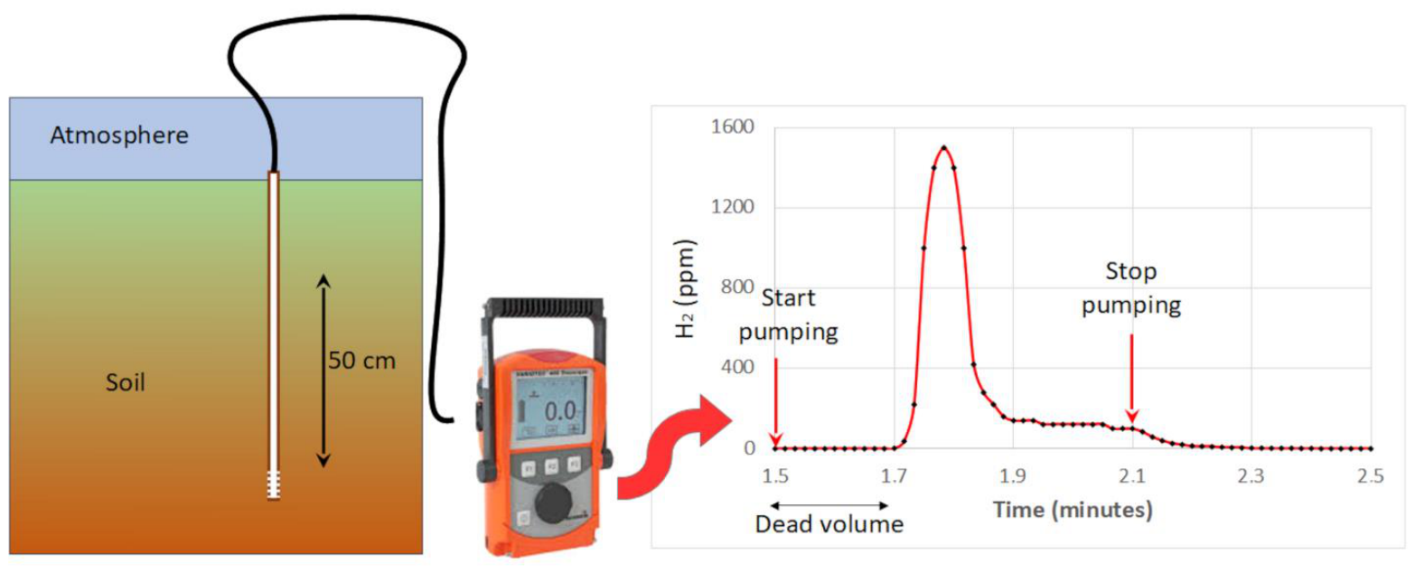
Today, it is also widely used for natural hydrogen exploration [3,4,5,6,7,8], as it is the first cheapest methodology allowing to define areas with some potential for a hydrogen system. However, like in other geological fields, its efficiency and reliability are often questioned (see [9,10] for example). The usual technique is measuring hydrogen concentration after drilling a borehole around 1 m deep (Figure 1, see [6] for details of this kind of measurement). A hydrogen detector is then connected to the hole, and the air present in soils is pumped out with possible traces of hydrogen [6]. The measurements may be punctual and instantaneous; one may be repeated several minutes later to check if there is any observed recharge at the same spot [11]. Also, a long-term monitoring (one or several months) may also be done, either pumping periodically the soil [7,8], or measuring the trace gas in a static mode [4,5]. Hydrogen in the soils may be measured alone or associated with other gas compounds (atmospheric compounds as the most abundant, CO, CO₂, He, hydrocarbon, olefins, etc.).

For any of these techniques, scientific discussions occur about possible artefacts (drill bit metamorphism generating artificial hydrogen, biological activity generating natural but superficial hydrogen, desorption of already trapped natural hydrogen, etc.) potentially killing the interest of the method. In order to distinguish these phenomena from a real active deep flow of hydrogen coming from a subsurface hydrogen system, we present a model associating hydrogen trapped in the soil sediments and a potential associated active deep flow. In this model, other processes of hydrogen generation (Drill Bit Metamorphism, i.e., DBM) and biological superficial hydrogen generation are not considered, even if their importance is also to be taken in consideration.

Natural Observations

Thousands of soil measurements are done each year to measure natural hydrogen. Figure 1 represents the usual way these measurements are performed: after the drilling of a borehole of about 1 m deep in the vadose zone of the soil (hole which may be done through rotating drilling bit or through percussive bit entrance), a tube is introduced inside the hole without any packer, and a hydrogen detector is linked to this tube through a pumping system, allowing to pump out the air present in the soil’s porosity and measure the traces of hydrogen in it. In the case of Figure 1, the detector is a Sewerin Variotech© with a pumping system flowing 50 L of gas per hour. In this figure, a hydrogen peak around 1500 ppm is measured during a pumping phase around 2.1 min.

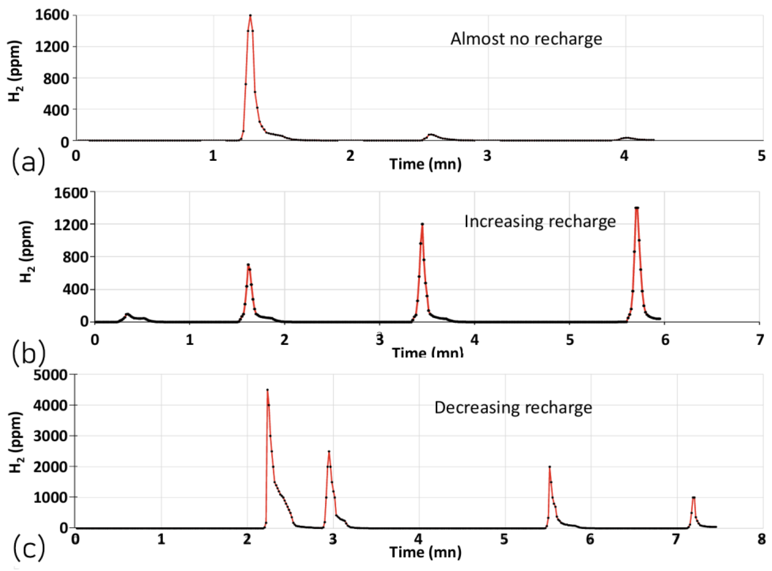
All the soils we studied here are mainly sandy, with some shales. This kind of soil is almost always similar in fairy circles, even if we deal here with a geological setting not related to a fairy circle but to the vicinity of a tectonic accident. It appears that hydrogen in soils may sometimes present a clear recharge after stopping and restarting the pump during several minutes [11], or remains absent for a long time after a single pumping (See [6] and Figure 2a). As presented in Figure 2b, the recharges may appear larger than the initial H₂ peak, but it is not always the case as shown in Figure 2c. These kinds of behavior occur in various geological contexts where natural hydrogen is measured through surface geochemistry, in both sedimentary and igneous rocks.

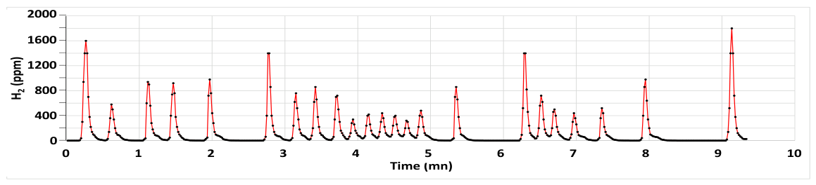
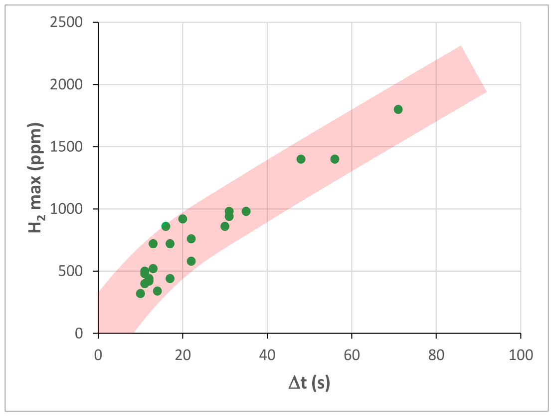
In some cases, it was possible to wait for a longer time and multiply the measurements as shown in Figure 3. In that case, it appears that the height of the peaks is qualitatively related to the time interval between two pumpings/measurements (Figure 4). These series of measurements were obtained along a major reactivated tectonic accident affecting continental formations. No fairy circle could be observed in this place or in its vicinity. It is important to notice that these observed recharges are generally observed in different places associated with faults, and very rarely in fairy circle measurements. It should be noted that the height of the peaks is not related to the duration of the experiment, but only to the time separating each pumping. A passive replenishment of the soil through simple diffusion of already present hydrogen would present a progressive decrease of the hydrogen pumped for each peak.

2. Modelling

The question we want to address with these data is the possibility to distinguish (or not) an active flow of natural hydrogen where we perform surface geochemistry measurements, from either hydrogen artefacts due to our drilling operation, or hydrogen trapped in the soil through adsorption in the grains of the soils.

In order to assess the behavior of the measured hydrogen as presented above, we present 3 different models, each of them representing a brick of a general modelling. Model A is a simple steady-state model of hydrogen diffusion through the porosity of the soils. Model B presents a transient hydrogen migration occurring through various pulses of natural hydrogen invading and leaving the soil’s porosity resulting from the consecutive pumpings of a measurement sequence. Model C presents the relative importance of adsorption/desorption processes at the scale of the soil minerals.

The following models assume that the air in soil porosity is static when there is no pumping. It follows that we only consider diffusion as a transfer mechanism of hydrogen in the porosity. The occurrence of a Darcean flow, which seems unprovable, would improve our conclusions about the presence or absence of active hydrogen seeping. As a matter of fact, a Darcean flow is much more efficient than diffusion for gas migration. The removal of hydrogen in the soil porosity would be then much quicker, implying that its presence has to be related to an active flow.

2.1. Model A (Figure 5): Steady State Hydrogen Migration

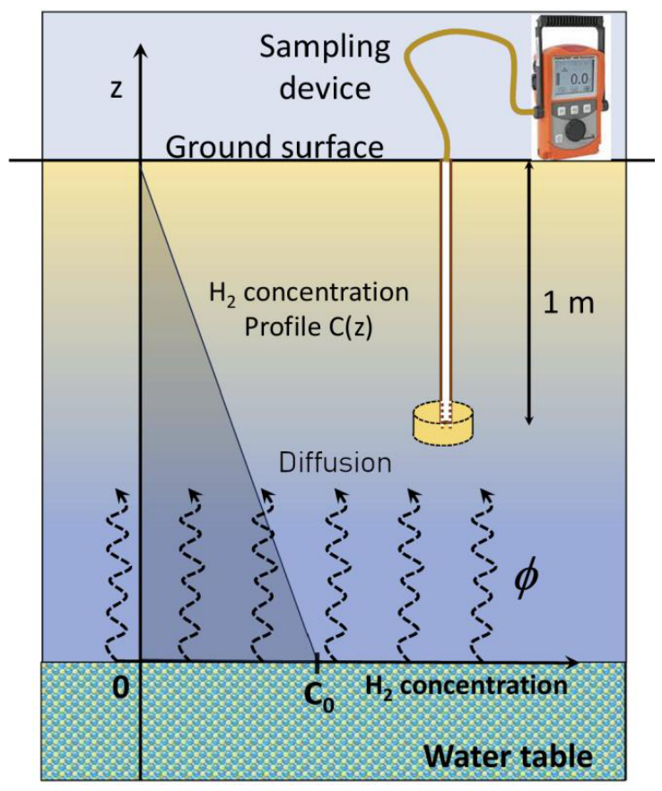
The objective of the first simple model is to estimate the spatial distribution of hydrogen concentration in the gas occupying the unsaturated subsurface interval (vadose zone with mainly air in the porosity). It is a 1D vertical model representing a column of homogeneous porous medium whose porosity is occupied by a perfectly connected free gas phase. The base of the column is placed at the top of the water table (piezometric level), and its top corresponds to the ground surface. The characteristic scale of this model is therefore metric to decametric. It is assumed that a flux φ of hydrogen emanating from a deep source is continuously supplied at the base of the column, and that no other hydrogen source, positive (generation) or negative (alteration), exists within the column. It is also assumed that the hydrogen concentration in the atmosphere (around 0.5 ppm [12]) is negligible, which imposes a zero-hydrogen concentration limit at the ground surface. This is always verified when putting a hydrogen detector on the surface of the ground: the concentration remains zero, even close to the vent of a drilled hole.

Figure 5. Representative diagram of model A.

Figure 5. Representative diagram of model A.

In the case where the hydrogen supply is sufficiently low to be entirely evacuated by diffusion in the gas phase, the hydrogen concentration profile in the gas phase at steady state is given by the following relation [13]:

$$C\left(z\right)=C_0{\displaystyle \frac{z-L}{L}}$$

(1)

where:

• z is the elevation relative to the top of the water table, in m
• $C_0$ is the hydrogen concentration in the gas phase at the base of the column, i.e., immediately above the top of the water table, in mol·m⁻³
• L is the depth of the top of the water table relative to the ground level, in m

The hydrogen flux φ in mol·m⁻²·s⁻¹ is then expressed by the following expression:

$$\phi =-D_{eff}{\displaystyle \frac{C_0}{L}}$$

(2)

where $D_{eff}$ is the effective gas-phase diffusivity in m²·s⁻¹. Different models to determine the ratio (where $D$ is the hydrogen diffusivity in air under the thermodynamic conditions of interest) are proposed in the literature [14]. This ratio is controlled by various soil parameters including porosity structure and soil humidity. The experimental determination of this ratio has been the subject of several studies [15,16]. Reference [15] reports that it can range from 0.05 to 0.35 at a depth between 50 cm and 1 m, depending on soil type and humidity conditions.

The maximum hydrogen flux ${\phi }_{max}$ that can be evacuated by diffusion is obtained in the extreme case where the free gas at the base of the unsaturated zone is entirely composed of hydrogen. In this case, we obtain:

$${\phi }_{max}=-{\displaystyle \frac{D_{eff}}{L}}.{\displaystyle \frac{{\rho }_{H2}}{M}}$$

(3)

where ${\rho }_{H2}$ is the hydrogen density (in kg·m⁻³) in the conditions of the experiment and M is the molar mass of hydrogen (in kg·mol⁻¹). A numerical application to an unsaturated column of 10 m height gives a maximum diffusive flux of about 15 mol·m⁻²·day⁻¹. If the rate of hydrogen emissions exceeds this limit value, a Darcy flow of free hydrogen is established, and when a steady state is reached, the gas phase is entirely composed of hydrogen throughout the column, a case not observed in the data reported here.

According to this model, it follows from (2)–(4) that a concentration measurement C_m (in mol·m⁻³) performed at a depth z_m theoretically allows the determination of the hydrogen flux ${\phi }_m$ using the following expression:

$${\phi }_m=-D_{eff}.{\displaystyle \frac{C_m}{z_m}}$$

(4)

It appears from previous studies [4,7,9] that hydrogen measurements in soils are not constant through time, indicating that this first model is an oversimplification of what is really observed, except if the steady state occurs rapidly enough considering the duration of the gas arrival. However, in a general case, steady-state model is not adequate for interpreting hydrogen concentrations in soils.

2.2. Model B (Figure 6): Transient Pulsing Hydrogen for Its Emission and Its Measurements

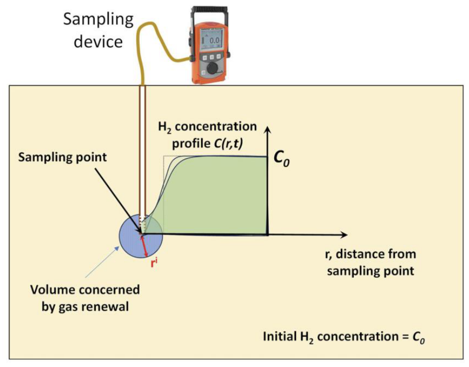
The objective of this second model is to estimate the spatiotemporal evolution of the free hydrogen gas concentration near the sampling point of the measurement device. This second model is time-dependent, in opposition with model A. The evolution of hydrogen concentration is modeled by considering a spherical problem centered on the sampling point, in an infinite medium (Figure 6). The characteristic scale of this model is centimetric to decimetric as the gas filling the porosity is supposed to be disrupted only a few centimeters to decimeters from the sampling point. The following assumptions are also made:

• At the initial moment of the measurement sequence while pumping the air from the soil, the hydrogen concentration C₀ in the free gas is uniform.
• Each ith sampling replaces a volume Vⁱ of free gas with pure air, within a spherical domain of radius rⁱ centered on the sampling point. We assume that each sample is taken instantly. This means that we ignore the flux of hydrogen through the envelope of the drainage volume during the pumping, and the effect of the pressure perturbations on the gas flow and local gas mixing during this period. This simplification results in a discontinuous concentration profile around the sampling point immediately after pumping, whereas dispersion is expected to smooth this profile in the field. This simplification was deemed acceptable considering our objective.

Figure 6. Representative diagram of Model B.

Figure 6. Representative diagram of Model B.

In accordance with what is generally accepted for gas flow in soils [17] and given that there was no wind during the measurements, we can assume that conditions are isobaric and isothermal during the small time intervals between two pumping periods. It follows that diffusion is the dominant process controlling the transfer of hydrogen in the gas phase [15,17]. Thus, the spatiotemporal evolution of the hydrogen concentration around the sampling point can be determined by solving the spherical diffusion equation [18]:

$${\displaystyle \frac{\partial C\left(r,t\right)}{\partial t}}=D_{eff }\left({\displaystyle \frac{{\partial }^{2}C\left(r,t\right)}{\partial r^2}}+{\displaystyle \frac{2}{r}}{\displaystyle \frac{\partial C\left(r,t\right)}{\partial r}}\right)$$

(5)

with the following initial and boundary conditions:

• $\forall t \le 0, \forall r \ge 0, C\left(r,t\right)=C_0$
• $\forall i\in \left[1,n\right],\forall r\in \left[0,r^i\right],C\left(r,t^i\right)=0$ which indicates that at each ith measurement, the concentration is reset to 0 within a sphere of radius rⁱ centered on the sampling point,

where r is the distance from the sampling point, t is time, n represents the number of samples taken during the measurement sequence, and tⁱ is the time of the ith sampling.

It is noted that the radius rⁱ and the sampled volume Vⁱ are related by the following equation:

$$r^i=\sqrt[3]{{\displaystyle \frac{3V^i}{4\pi \theta }}}$$

(6)

with θ corresponding to the soil porosity. The average concentration $C_m^i$ of hydrogen in the gas sampled at the ith measurement is obtained by integrating the concentration immediately before sampling within the volume of gas renewed by pumping:

$$C_m^i={\displaystyle \frac{3}{{\left(r^i\right)}^3}}{\displaystyle \underset{r=0}{\overset{r^i}{\int }}}{r}^2.C\left(r,t^i\right).dr$$

(7)

With this model, it is possible to simulate a succession of samplings and calculate the sequence of average concentrations measured by solving Equation (6) with the following data and parameters:

• The diffusion coefficient of hydrogen in soil gas $D_{eff}$,
• The hydrogen concentration in soil gas before the start of measurements, assumed to be uniform, $C_0$. This corresponds to a chosen limit condition,
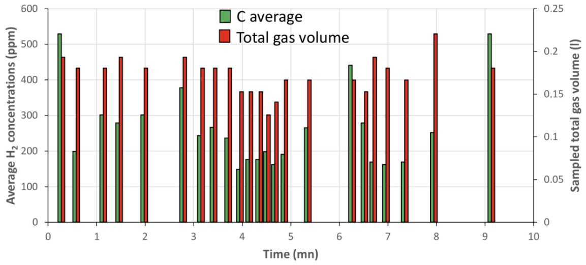
• The list of sampling times and sampled volumes as presented for example in Figure 3, ${\left[t_i\right]}_{i=1}^n$ and ${\left[V_i\right]}_{i=1}^n$. As we consider each pumping and associated measurements instantaneous, we use for the modelling the average concentrations measured for each peak presented in Figure 3.

• Application to the Figure 3 measurement series

Here, we aim to interpret a sequence of field measurements to estimate the concentration of hydrogen in soil gas before it was disrupted by the measurements. To do this, we proceed by inverting the model B described above, seeking to adjust the effective diffusion coefficient $D_{eff}$ and the concentration $C_0$ so that the average hydrogen concentrations measured during each sampling are best approximated by the simulated values.

The data contain 23 measurements taken at the same sampling point, at time intervals of 10 to 71 s, as represented in Figure 7. The total duration of the experiment is slightly above 9 min. The sampling times ${\left[t_i\right]}_{i=1}^{23}$, sampled volumes ${\left[V_i\right]}_{i=1}^{23}$, and average concentrations ${\left[C_m\right]}_{i=1}^{23}$ were measured. Moreover, an initial pumping was taken a few tens of seconds before the recorded measurements. The time of this sampling t₀, as well as the sampled volume V₀, were not measured and constitute two other model adjustment parameters, in addition to $D$_eff and C₀.

The pumping sequence is simulated by solving Equation 6 using an explicit finite difference scheme. The chosen time step is 0.09 s. The simulated domain is a sphere with a radius of 60 cm, centered on the sampling point (Figure 6). The radius is discretized into steps of 3 mm.

The simulation of the measurement sequence is integrated as a direct model in an inversion loop, where the parameters (D_eff, C₀, θ, t₀, V₀) are adjusted so that the average calculated concentrations $C_{mCalc}^i$ best approximate the measured values in the least-squares sense, i.e., by minimizing ${\displaystyle {\sum }_{i=1}^{23}}{\left(C_m^i-C_{mCalc}^i\right)}^2$. The inversion is performed using the “minimize” function from the Python library SciPy v1.18.0, then refined by systematically exploring the parameter space around the solution proposed by the inversion.

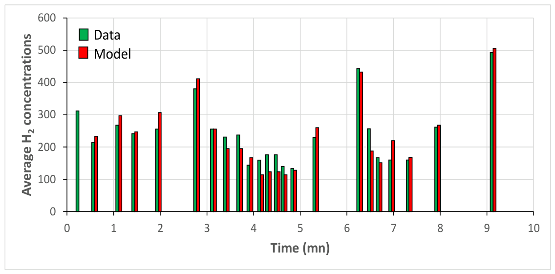
The best fit (Figure 8) is obtained for the following parameter values:

• D_eff = 6.2 × 10⁻⁶ m²·s⁻¹
• C₀ = 1715 ppm
• θ = 11%
• T₀ = 53 s
• V₀ = 394 cm³

Applying a hydrogen diffusion coefficient of 6.5 × 10⁻⁵ m²·s⁻¹ in air under normal conditions yields a ${\displaystyle \frac{D_{eff}}{D}}$ value of 0.095, which lies within the acceptable range of values [0.05; 0.35] [15]. However, the porosity of 11% is lower than the actual soil porosity. The analysis of the quality of the inversion showed that a large range of solutions yield a mean square distance that is less than 10% different from the minimum mean square distance. All these solutions show a C₀ value that ranges from 1600 to 2500 ppm and a porosity that ranges from 10% to 30%. This means that solutions with more realistic porosities are also acceptable. Finally, it is verified that the calibrated values of T₀ and V₀ are consistent with expected orders of magnitude.

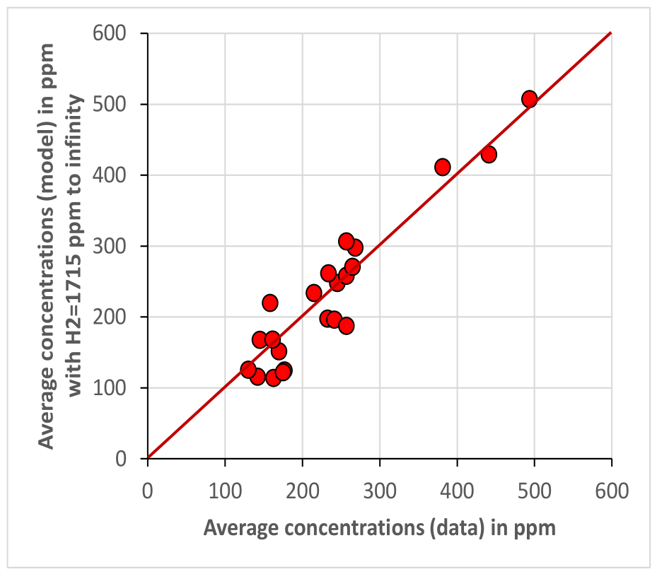
The good quality of the fit is also illustrated by Figure 8 and Figure 9 thus lending credibility to the adopted model. However, due to its simplifications and parameter uncertainties, this model cannot accurately predict the baseline hydrogen concentration in the soil. Nevertheless, it shows that a baseline concentration of at least 1600 ppm of hydrogen in the gas-filled porosity of the soil before the start of the measurement is necessary to explain the observed results.

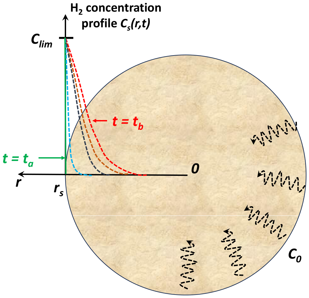
2.3. Model C: Adsorption/Desorption of Hydrogen in Soil Grains (Figure 10)

Finally, it was decided to test the importance of possible absorption/desorption of hydrogen by the solid phase of a soil. This third model is proposed to study the kinetics of hydrogen exchange through absorption/desorption between the solid phase and the free gas phase [19]. This model operates on a sub-millimeter scale, whereas models A and B operate at the meter and decimeter scales respectively. Its objective is to analyze under what conditions hydrogen could remain adsorbed in the soil for several days following the occurrence of a temporary hydrogen emission.

Figure 10. Representative diagram of model C showing a soil grain and its internal hydrogen concentration profile over time. Dashed arrows represent diffusion, and colored lines represent successive concentration profiles.

Figure 10. Representative diagram of model C showing a soil grain and its internal hydrogen concentration profile over time. Dashed arrows represent diffusion, and colored lines represent successive concentration profiles.

The model C scenario represents a soil initially free of hydrogen. At this stage, the free gas phase is assumed to consist of pure air. A temporary hydrogen emission is modeled over a time interval $\left[t_a,t_b\right]$, assuming that at time $t_a$, the air is instantaneously replaced by a mixture of air and hydrogen, with the hydrogen concentration $C_0$ remaining constant during $\left[t_a,t_b\right]$. When the emission ends, at ${t=t}_b$, the porosity is instantaneously filled with air maintained at an infinitesimal hydrogen concentration through continuous renewal. The partial pressure of hydrogen in the soil porosity during the entire emission period is denoted as $P_{H_2}$.

The solid phase of the soil is represented as an assembly of grains. These grains are modeled as a nanoporous material in which hydrogen molecules can migrate by diffusion and adsorb according to the Langmuir model. The effective diffusion coefficient in the grain is denoted as $D_s$ (in m²·s⁻¹), and the maximum absorption capacity (theoretically reached at infinite hydrogen pressure) of the grains at the soil temperature is denoted as $C_{Max}$ (in mol·m⁻³). The grains are represented as spheres with a radius $r_s$, and their radial hydrogen concentration profile, expressed in mol·m⁻³, is denoted as $C_s\left(r,t\right)$.

The spatiotemporal evolution of the hydrogen concentration in the grain $C_s\left(r,t\right)$ is the solution to the spherical diffusion problem presented in Equation (5). The initial and boundary conditions for this new problem are as follows:

• $\forall t\in \left[t_a,t_b\right],C_s\left(r_s,t\right)=C_{lim}\left(P_{H_2}\right)$
• $\forall t<t_a,\forall r\le r_s,C_s\left(r_s,t\right)=0$
• $\forall t>t_b,C_s\left(r_s,t\right)=0$

The adsorption of hydrogen by soils has received little, if any, study. However, the adsorption of hydrogen in geological storage has been well studied, with results showing that the Langmuir model of hydrogen adsorption on geological materials is well suited to reservoir pressure and temperature conditions [16,20,21]. We will therefore assume that the Langmuir model of hydrogen adsorption in soil minerals also applies under standard conditions. Following this assumption, the grain surface is in equilibrium with soil gas at all times. Let $C_{lim}\left(P_{H_2}\right)$ represent the gas concentration (in mol·m⁻³) that can be adsorbed at equilibrium by the grain, at the temperature of the studied system, and at the partial pressure $P_{H_2}$ of hydrogen in the free gas.

Assuming Langmuir adsorption, $C_{lim}\left(P_{H_2}\right)$ is expressed as follows:

$$C_{lim}\left(P_{H_2}\right)= C_{Max}{\displaystyle \frac{b. P_{H_2}}{1+b.P_{H_2}}} \cong C_{Max} . C_0$$

(8)

where $b$ and $C_{Max}$ are characteristic properties of the material constituting the grain, representing the Langmuir parameter (in bar⁻¹) and the maximum adsorption capacity at the temperature of the studied system, expressed here in mol·m⁻³, respectively.

Finally, $K\left(t\right)$, the total amount of hydrogen adsorbed by the soil, expressed in mol·g⁻¹ (moles per gram of solid), is obtained by integrating the adsorbed gas concentration with respect to the distance from the center of the grains:

$$K\left(t\right)={\displaystyle \frac{1}{\rho }}{\displaystyle \frac{3\left(1-\theta \right)}{4\pi r_s^3}}{\displaystyle \underset{r=0}{\overset{r_s}{\int }}}{4\pi r^2.C}_s\left(r,t\right).dr$$

(9)

where $\rho$ represents the grain density in g·m⁻³.

$K\left(t\right).\rho$ can be normalized by $C_{lim}\left(P_{H_2}\right)$ to obtain the amount of hydrogen adsorbed by the grains, normalized by the maximum possible amount obtained at equilibrium (dimensionless):

$$k\left(t\right)={\displaystyle \frac{\rho K\left(t\right)}{C_{lim}\left(P_{H_2}\right)}}$$

(10)

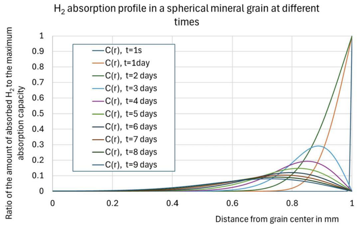
The Figure 11 shows an example of the time evolution (from 0 to 9 days) of the amount of hydrogen adsorbed by the soil during and after a 2-days hydrogen emission, for the following parameter values of the model:

• r_s = 1 mm
• D_s = 4 × 10⁻¹⁴ m²·s⁻¹
• T_a = 0
• T_b = 172,800 s (2 days)

We can see that at the beginning of the stopping of H₂ emission, the H₂ concentration curve inside the grain is monotonous, decreasing with the distance to the surface of the grain. After 2 days, corresponding to the removal of free hydrogen in the gas of the soil, hydrogen concentration is higher in the central part of the grain whereas it decreases close to the surface of the grain.

• Numerical Application

According to our model, the dynamics of the evolution of the amount of hydrogen adsorbed by the soil are controlled by the grain size and diffusion coefficient $D_s$. The absolute amount of hydrogen adsorbed per unit mass of soil, on the other hand, depends on the duration and hydrogen concentration of the emissions and the adsorption capacity of the grains $C_{Max}$. The specific surface of the soil grains is generally considered as an important parameter influencing greatly the amount of adsorbed gas in the case of a kinetic process. In the presence of a thermodynamic equilibrium, this parameter does not have any effect on the amount of adsorbed gas; only the capacity of adsorption of the solid will control it. As the diffusion coefficients in solids as D_s are extremely low, mainly at surface conditions of temperature, this implies the need of too long times for reaching an equilibrium. Then, the specific surface area SSA expressed in m²·m⁻³, plays an important role. In our model, it is considered indirectly through the grain radius which is related to the SSA as follows:

$$r_s={\displaystyle \frac{3\left(1-\theta \right)}{SSA}}$$

(11)

$D_s$ and $C_{Max}$ are properties that have been very little studied for granular constituents under the pressure and temperature conditions of soils, and most measurements of these properties were conducted in the conditions of deep underground repositories or storages [7,19,22,23,24]. Laboratory acquisition of these data for soils would be necessary to improve our understanding of soil gas measurements. As our objective is to establish the conditions under which hydrogen can possibly remain adsorbed for several days, we focused on the lowest $D_s$ values and the highest $C_{Max}$ values reported in the literature, since the model detailed below showed that low $D_s$ and high $C_{Max}$ are necessary in order to keep hydrogen adsorbed for several days.

Table 1. Some values of absorption capacity and diffusion coefficients in geologic material from the literature; bold is used for values reported in the papers; the last column reports values extrapolated for soil with a hydrogen concentration in the porosity of 1000 ppm. *: inferred from [23,24,25].

Sample Origin	T (K)	P (bar)	Plangmuir (bar−1)	Qe (mg·g−1)	Qmax (mg·g−1)	Qmax (µmol·g−1)	D (m2·s−1)	Ref.	Clim (mg H2·g−1)
Diverse minerals	600						[1 × 10−16; 1 × 10−12]	Lodhia *
Organic rich shale, Jordanian Oil Source Formation, well 1	303	15	0.073	0.73	1.4	698	2.6 × 10−18	Alanazi	0.051
Organic rich shale, Jordanian Oil Source Formation, well 2	303	15	0.025	0.06	0.2	110	1.5 × 10−17	Alanazi	0.0027
Clay rock, COX pure	301		0.036		3.06	1530		Bardelli	0.055
Clay rock, COX raw	301		0.073		1.12	560		Bardelli	0.041

presents some examples of these high values reported in the literature. The two Jordanian shales and the two clay rocks were characterized at ambient temperature conditions, which implies that adsorption capacity does not need to be corrected for soil temperature in the section below.

Instead of using a direct approach, we analyze the conditions under which hydrogen could remain adsorbed in soil in significant quantities several days after an emission.

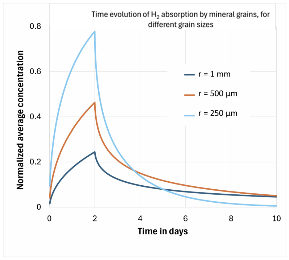
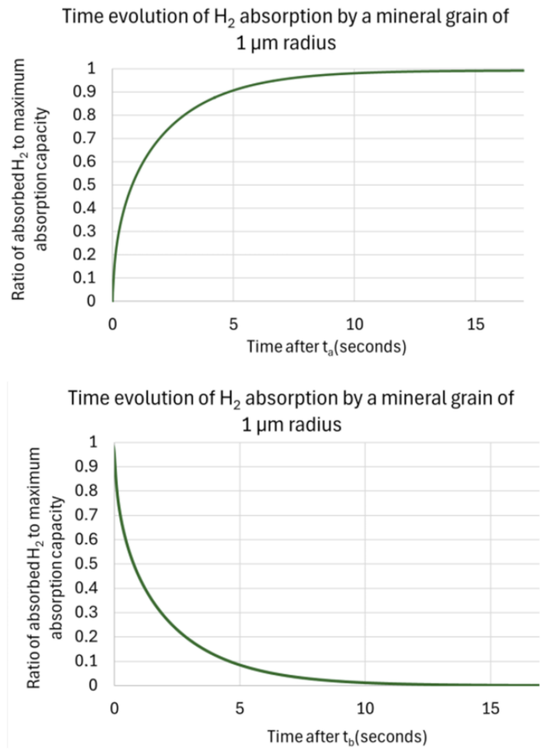
A sensitivity study of the results to the model parameters showed us that the evolution dynamics primarily depend on the ratio $D_s/{r_s}^2$, similarly to what can be demonstrated in the simple case of a sphere with an initial concentration of zero, on the surface of which a concentration C_lim is applied at $t\ge 0$ [3]. Thus, the pairs $\left(D_s,r_s\right)$ that satisfy ${\displaystyle \frac{D_s}{r_s^2}}=8\times {10}^{-8}$ all exhibit the evolution dynamics shown in Figure 11. However, for a given diffusion coefficient $D_s$, the absorption and desorption dynamics are directly controlled by the grain size. This is illustrated by Figure 12 and Figure 13 which show the dynamics of absorption and desorption for $D_s=4\times {10}^{-14}$ m·s⁻¹ and 4 different grain radii from 1 µm to 1 mm. Total absorption/desorption is obtained in 10 s for small grains with 1 µm radius, while it takes more than 2 days for grain radii above 250 µm.

It remains to evaluate the quantity of adsorbed hydrogen and relate it to the air volume of the porosity to assess whether the release of a portion of the adsorbed hydrogen into the porosity could significantly increase the hydrogen concentration in the pore space. Assuming that the maximum quantity of adsorbed hydrogen K(t) was instantaneously released into the porosity initially filled with pure air, the hydrogen concentration in the porosity would reach the following molar concentration C_f:

$$C_{f=}{\displaystyle \frac{C_{lim}\left(P_{H_2}\right).k\left(t\right)}{M.\frac{\theta }{1-\theta }\frac{1}{\rho }\frac{{10}^6}{0.0224}}}$$

(12)

where $M$ is the molar mass of hydrogen and the term $\left(M.{\displaystyle \frac{\theta }{1-\theta }}{\displaystyle \frac{1}{\rho }}{\displaystyle \frac{{10}^6}{0.0224}}\right)$ represents the number of µmol of air per 1 g of mineral, assuming that air and hydrogen are ideal gases.

Using the same numerical application as that illustrated by Figure 12 and Figure 13, we obtain $C_f=784.k\left(t\right)$ (in ppm), given the parameters below:

• $P_{H_2}$ = 1 × 10⁻³ bars
• $C_{lim}$ = 0.05 µg·g⁻¹ (0.032 mol·m⁻³)
• $\rho$ = 2600 kg·m⁻³
• $\theta$ = 65%

This means that 4 days after the cessation of hydrogen emanation, and for parameters defined here above, especially grain agglomerate radii around 500 µm, the hydrogen concentration in the pore space would reach around 400 ppm if all the adsorbed hydrogen were instantaneously transferred into the pore space. However, the desorption rate is actually very low at this time, at around 1–2% per day. This increases the hydrogen concentration in the porosity by only 4–8 ppm per day. In practice, the soil is made of grains with very dispersed radii, with the smallest grains desorbing within a few seconds after the H₂ emission stops, whereas the biggest ones could retain hydrogen for a few days but desorb at a very low rate.

Figure 12 shows the same behavior, indicating that the amount of hydrogen adsorbed after two days of hydrogen emission is larger for smaller grain sizes, but decreases more quickly.

Finally, this model shows that adsorption and desorption may interact with the diffusion process described in Model B, as both diffusion and adsorption operate on the same timescale for micrometric grains. A version of model B that is coupled with an adsorption and desorption calculation shows that, immediately after pumping, hydrogen can desorb and can contribute to recharge the gas phase around the sampling point. Just after, when the diffusion front arrives, hydrogen concentration in the gas phase increases and adsorption recharges the grains. This model is not presented in detail here, as the increased number of parameters makes inversion difficult. However, direct calculations show that adsorption could impact the system response in the case of very high adsorption capacity and very small grains. With the diffusion coefficient D = 4 × 10⁻¹⁴ m²·s⁻¹ used here above, a uniform grain size of 1 µm and an extreme adsorption capacity of 0.05 µg·g⁻¹, adsorption and desorption interact during the three first pumpings, but adsorbed hydrogen is totally removed around the sampling point afterwards. Given these values which are very favorable for significant adsorption at the time scale of a few seconds, adsorption cannot solely explain the repeated recharge observed over more than 3 successive pumpings.

3. Discussion

Model A shows us that hydrogen emission up to a few tens of grams per square meter per day at the top of the water table results, when a steady state is reached, in a hydrogen concentration in the pores that varies linearly from the top of the water table to a negligible value at ground level.

Furthermore, situations are observed in which repeated measurements of hydrogen concentration, carried out at a depth of 1 m using an aspiration detector, show that the hydrogen concentration remains stable. The example presented in this work involves about twenty measurements taken at short intervals of one to a few tens of seconds. The results obtained show that about ten seconds are sufficient to significantly indicate a modelled recharge in the pumping zone with hydrogen after each sampling. Model B shows that this rapid increase in concentration in the pumping zone can only be explained by the diffusion of hydrogen from the peripheral zone, which is undisturbed by the measurements, toward the pumping zone, in an environment where the initial hydrogen concentration is uniformly non-zero, comparable to the conditions of a continuous hydrogen supply at the top of the water table as described by Model A.

Model C examines whether an absorption-desorption process in a porous medium, where the hydrogen concentration in the pores before the measurements is almost zero, could also be considered to explain these observations. In this alternative scenario, the absence of hydrogen in the porosity before the measurements is due to the lack of hydrogen supply at the base of the model. However, the presence of hydrogen adsorbed by the minerals could be explained by a hydrogen emission that has now ceased. Model C shows that minerals can only sustainably adsorb hydrogen in significant quantities if their absorption capacity is very high (we used the highest values reported in the literature) and if the grain size is of the order of 1 mm diameter. Under these conditions, the hydrogen exchange rates between the mineral and the porosity are very low and cannot explain the levels of hydrogen concentration observed during the samplings. However, it can be considered that the mechanical disturbance of the soil during drilling causes the breaking of the biggest grains which would temporarily increase the desorption rate, triggering a short-term release of the gas adsorbed by the newly formed fine grains. However, it is difficult to explain a lasting and significant increase in hydrogen concentration in the porosity using this mechanism, due to the limited number of grains crushed during the drilling, compared to the volume of gas investigated by the samplings.

These 3 models allow to assess for the first time the significance of surface geochemical hydrogen measurements. More work and more quantitative parameters would be necessary in order to better constrain the reliability of this kind of measurements. However, it is possible to consider that without any observable hydrogen recharge of the pore volume concerned by the samplings at the time scale of minutes, it is very difficult to conclude for an active hydrogen flux when the measurements occur. More precisely, in order to avoid any ambiguity with apparent recharge linked to the re-equilibration of hydrogen in soils after each pumping, the apparent recharge peaks need not to be decreasing with time but associated with other parameters as the time interval between each pumping, as shown Figure 3. The variability of the grain sizes induces that for the very small grains (shales for example), the adsorption may be large, even during a short time, but the desorption should occur extremely rapidly. On the opposite, for large grains, a pulse of hydrogen will be trapped for a long time, but its emission through desorption will allow very low concentrations in the air of the soil, around 10 ppm, which may be considered negligeable during surface measurements, which become significant for several hundreds of ppm.

3.1. Drill Bit Metamorphism (DBM) and Hydrogen Generation

Drill Bit Metamorphism (DBM) is a well-documented phenomenon occurring during the drilling of oil and gas wells. The production of hydrogen is associated with the interaction between water and drilling tools, often accompanied by the generation of carbon compounds such as carbon monoxide and olefins. Detecting the presence or absence of these compounds (H₂, CO, CO₂, olefins) serves as an indicator of DBM. In surface geochemical studies, if no water is present in the soil (e.g., in arid regions), no artificial hydrogen generation can occur. However, debates about potential human-induced artifacts persist, even when high hydrogen concentrations are detected [5,9]. These works demonstrate experimentally the possible importance of drill bit metamorphism for generating very large concentrations of hydrogen in analyzed soils. This artificial hydrogen generation may be due either to water reduction with iron (as observed during the drilling of deeper wells at high temperature) or to the mechanical breakage of water molecules associated with the breakage of soil minerals. In the case of hydrogen artificially generated during drilling, the consequence may be also evaluated through the models presented above: the departure of hydrogen will be then controlled by air diffusion and solid diffusion, the later for the adsorption/desorption process. Air diffusion will remove rapidly the generated gases, whereas adsorption/diffusion will present a very limited effect, due to the very short time involved for hydrogen trapping through this process.

Conversely, when hydrogen recharge is observed over several minutes or hours, the model suggests that the hydrogen in the soil cannot be attributed to either human artifacts or residual adsorption in soil grains. It is essential to note that this conclusion is based on specific modeling conditions. Variations in physical parameters, such as differing grain sizes due to soil grain clustering, could alter the quantification. Additionally, the model does not account for the depth at which hydrogen generation occurs. For instance, in cases of shallow bacterial hydrogen production (as described by [9]), the model would indicate active hydrogen flow, even if unrelated to deeper subsurface hydrogen “kitchens” potentially linked to producible gas accumulations.

3.2. Hydrogen Flux Quantification

In our models, the hydrogen concentration at the piezometric level is optimized between 784 and 1715 ppm. Assuming a depth of 4 m for this level and an effective diffusivity of 6.2 × 10⁻⁵ m²·s⁻¹, this results in a hydrogen flux ranging from 10⁻³ to 2.3 × 10⁻³ m³·m⁻² per day. These values are approximations and highly dependent on the piezometric level’s depth. They are, even high, approximately one order of magnitude lower than the fluxes calculated from long-term monitoring in the São Francisco Basin, Brazil [7,26].

To differentiate between superficial and deep gas flows observed in soils, it has been proposed to measure helium concentrations [11]. A positive helium concentration anomaly exceeding atmospheric levels (5.24 ppm) would unequivocally indicate a deep gas flow, as helium cannot be generated in significant quantities within soils nor adsorbed and desorbed onto mineral surfaces [27].

3.3. Intermittent Hydrogen Flow Observations

A common observation involves detecting a clear recharge of hydrogen over several hours on one day, followed by a return to the same location the next day, where no hydrogen anomaly is observed, even during the initial pumping. This can be explained by our model and previous findings, which indicate that hydrogen seepage in soils is not constant [7], as it is often observed for both onshore and offshore petroleum. Active hydrogen flow typically occurs for a maximum of a few days, after which hydrogen migration ceases at the same spot.

4. Conclusions

This study introduces a model that attempts to distinguish active hydrogen flow in soils from artificially generated hydrogen during drilling or from adsorbed hydrogen in soil grains. The quantification of hydrogen migration suggests that observing a recharge within a short timeframe (minutes or hours) is indicative of an active hydrogen flux. This is mainly the case here where the measurements were done in the vadose zone of the soils, where the permeability is quite large (as the soil is sandy) and that it is mainly filled with air, avoiding any trapping of gas due to low permeability. The absence of such recharge would imply either artificially generated hydrogen or trappeded hydrogen within the soil. However, this observation alone cannot differentiate between deep hydrogen production in subsurface “kitchens” and shallow hydrogen generation via biological processes.

To confirm a deep origin of hydrogen, measuring associated helium concentrations in soil is a reliable method. Helium anomalies exceeding atmospheric levels (5.24 ppm) cannot be attributed to superficial events, whether natural or human-induced. Field measurements or laboratory analyses of collected gas samples provide a robust technique for verifying surface gas anomalies linked to active gas flow, as helium does not adsorb onto mineral surfaces.

By combining observations such as hydrogen recharge, and adding soil quality analysis, and helium measurements (beyond the scope of this work), misinterpretations of hydrogen origins in soils can be minimized. Following these precautions during surface geochemical surveys ensures the accurate identification of hydrogen anomalies, reducing the likelihood of misidentifying artifacts, which, while possible, are now easily recognizable.

References

1. Cohen, D.; Bowell, R. Exploration Geochemistry. In Treatise on Geochemistry, 2nd ed.; Elsevier: Amsterdam, The Netherlands, 2013; Volume 13, pp. 623–650. [Google Scholar] [CrossRef] [Scilit]
2. Schumacher, D. Surface Geochemical Exploration for Petroleum. In Exploring for Oil and Gas Traps; American Association of Petroleum Geologists (AAPG): Tulsa, OK, USA, 1999. [Google Scholar] [CrossRef] [Scilit]
3. Lodhia, B.H.; Peeters, L.; Frery, E. A review of the migration of hydrogen from the planetary to basin scale. J. Geophys. Res. Solid Earth 2024, 129, e2024JB028715. [Google Scholar] [CrossRef] [Scilit]
4. Davies, K.; Frery, E.; Giwelli, A.; Esteban, L.; Keshavarz, A.; Iglauer, S. A natural hydrogen seep in Western Australia: Observed characteristics and controls. Sci. Technol. Energy Transit. 2024, 79, 48. [Google Scholar] [CrossRef] [Scilit]
5. Davies, K.; Haines, P.W.; Thomas, C.; Normore, L. Natural hydrogen soil gas emissions near Harvey, Perth Basin: A comparative study of survey methods. Sci. Technol. Energy Transit. 2025, 80, 46. [Google Scholar] [CrossRef] [Scilit]
6. Larin, N.; Zgonnik, V.; Rodina, S.; Deville, E.; Prinzhofer, A.; Larin, V.N. Natural molecular hydrogen seepages associated with surficial, rounded depression on the European craton in Russia. Nat. Resour. Res. 2015, 24, 363–383. [Google Scholar] [CrossRef] [Scilit]
7. Moretti, I.; Prinzhofer, A.; Françolin, J.; Pacheco, C.; Rosanne, M.; Rupin, F.; Mertens, J. Long-term monitoring of natural hydrogen superficial emissions in a brazilian cratonic environment. Sporadic large pulses versus daily periodic emissions. Int. J. Hydrogen Energy 2020, 46, 3615–3628. [Google Scholar] [CrossRef] [Scilit]
8. Prinzhofer, A.; Moretti, I.; Françolin, J.; Pacheco, C.; D’Agostino, A.; Werly, J.; Rupin, F. Natural hydrogen continuous emission from sedimentary basins: The example of a Brazilian H2-emitting structure. Int. J. Hydrogen Energy 2019, 44, 5676–5685. [Google Scholar] [CrossRef] [Scilit]
9. Etiope, G.; Ciotoli, G.; Ben, E.; Mazzoli, C.; Röckmann, T.; Sivan, M.; Squartini, A.; Laemmel, T.; Szidat, S.; Haghipour, N.; et al. Surprising concentrations of hydrogen and non-geological methane and carbon dioxide in the soil. Sci. Total Environ. 2024, 948, 174890. [Google Scholar] [CrossRef] [Scilit] [PubMed]
10. Halas, P.; Dupuy, A.; Franceschi, M.; Bordmann, V.; Fleury, J.-M.; Duclerc, D. Hydrogen gas in circular depressions in South Gironde, France: Flux, stock, or artefact ? Appl. Geochem. 2021, 127, 104928. [Google Scholar] [CrossRef] [Scilit]
11. Prinzhofer, A.; Rigollet, C.; Lefeuvre, N.; Françolin, J.; Valadao de Miranda, P.E. Marica (Brazil), the new natural hydrogen play which changes the paradigm of hydrogen exploration. Int. J. Hydrogen Energy 2024, 62, 91–98. [Google Scholar] [CrossRef] [Scilit]
12. Patterson, J.D.; Aydin, M.; Miranda, M.H.; Saltzman, E.S. Atmospheric H2 variability over the past 1,100 years. Nature 2026, 650, 898–902. [Google Scholar] [CrossRef] [Scilit] [PubMed]
13. Cussler, E.L. Diffusion: Mass Transfer in Fluid Systems; Cambridge University Press: Cambridge, UK, 2009. [Google Scholar]
14. Shen, L.; Chen, Z. Critical review of the impact of tortuosity on diffusion. Chem. Eng. Sci. 2007, 62, 3748–3755. [Google Scholar] [CrossRef] [Scilit]
15. Laemmel, T.; Maier, M.; Schack-Kirchner, H.; Lang, F. An in situ method for real-time measurement of gas transport in soil. Eur. J. Soil Sci. 2017, 68, 156–166. [Google Scholar] [CrossRef] [Scilit]
16. Wang, H.; Yang, E.; Dong, C.; Chen, S.; Liu, B.; Bai, J.; Sun, N.; Qu, M.; Liu, Y. Investigating the adsorption and transport behavior of hydrogen in underground hydrogen storage via molecular simulation. Int. J. Hydrogen Energy 2026, 207, 153541. [Google Scholar] [CrossRef] [Scilit]
17. Scanlon, B.R.; Nicot, J.P.; Massmann, J.W. 8 Soil Gas Movement in Unsaturated System. Soil Phys. Companion 2001, 297. [Google Scholar]
18. Carslaw, H.S.; Jaeger, J.C. Conduction of Heat in Solids; Oxford at the Clarendon Press: Oxford, UK, 1959. [Google Scholar]
19. Alanazi, A.; Abid, H.; Bawazeer, S.A.; Aljeban, N.; Abu-Mahfouz, I.S.; Keshavarz, A.; Iglauer, S.; Hoteit, H. Hydrogen and carbon dioxide kinetic adsorption and diffusion behavior into organic-rich shale: Implications of mineralogy and organic content. Energy Fuels 2024, 38, 23009–23024. [Google Scholar] [CrossRef] [Scilit]
20. Liu, A.; Liu, S. Hydrogen sorption and diffusion in coals: Implications for hydrogen geo-storage. Appl. Energy 2023, 334, 120746. [Google Scholar] [CrossRef] [Scilit]
21. Zhang, Q.; Masoudi, M.; Sun, L.; Zhang, L.; Yang, L.; Song, Y.; Hassanpouryouzband, A. Hydrogen and cushion gas adsorption–desorption dynamics on clay minerals. ACS Appl. Mater. Interfaces 2024, 16, 53994–54006. [Google Scholar] [CrossRef] [Scilit] [PubMed]
22. Bardelli, F.; Mondelli, C.; Didier, M.; Vitillo, J.G.; Cavicchia, D.R.; Robinet, J.C.; Leone, L.; Charlet, L. Hydrogen uptake and diffusion in Callovo-Oxfordian clay rock for nuclear waste disposal technology. Appl. Geochem. 2014, 49, 168–177. [Google Scholar] [CrossRef] [Scilit]
23. Demouchy, S. Diffusion of hydrogen in olivine grain boundaries and implications for the survival of water-richzones in the Earth’s mantle. Earth Planet. Sci. Lett. 2010, 295, 305–313. [Google Scholar] [CrossRef] [Scilit]
24. Kohlstedt, D.; Mackwell, S. Diffusion of hydrogen and intrinsic point defects in olivine. Z. Für Phys. Chem. 1998, 207, 147–162. [Google Scholar] [CrossRef] [Scilit] [PubMed]
25. Demouchy, S.; Mackwell, S. Mechanisms of hydrogen incorporation and diffusion in iron-bearing olivine. Phys. Chem. Miner. 2006, 33, 347–355. [Google Scholar] [CrossRef] [Scilit]
26. Cathles, L.; Prinzhofer, A. What Pulsating H2 Emissions Suggest about the H2 Resource in the Sao Francisco Basin of Brazil. Geosciences 2020, 10, 149. [Google Scholar] [CrossRef] [Scilit]
27. Feldman, J.; Paul, M.; Xu, G.; Rademacher, D.X.; Wilson, J.; Nenoff, T.M. Effects of natural zeolites on field-scale geologic noble gas transport. J. Environ. Radioact. 2020, 220–221, 106279. [Google Scholar] [CrossRef] [Scilit] [PubMed]
Figure 1. Principle of hydrogen surface geochemical measurements, using a detector with an integrated pumping device.
Geosciences 16 00364 g001
Figure 2. 3 different spots where H2 recharge has been checked for several minutes after the first peak. The measurements were done with a Variotech© instrument. (a) Almost no recharge, (b) Increasing recharge, (c) Decreasing recharge.
Geosciences 16 00364 g002
Figure 3. 23 consecutive measurements of H2 peaks in a 1 m-deep hole, obtained with a Variotech© instrument. The black points are the measured values, the red lines the interpolations between measurements.
Geosciences 16 00364 g003
Figure 4. Correlation between the maximum concentrations measured for each peak presented in Figure 3, and the time separating the peak from the previous one. Green dots: measured values. Pink area: qualitative correlation trend.
Geosciences 16 00364 g004
Figure 7. Representation of the analyzed measurement sequence. In red, the amount of total gas sampled in liters; in green, the average molar concentration for each peak measured in ppm.
Geosciences 16 00364 g007
Figure 8. Sequence of measured (in green) and calculated (in red) average concentrations after model parameter calibration.
Geosciences 16 00364 g008
Figure 9. Correlation between measured and calculated average concentrations after model parameter calibration.
Geosciences 16 00364 g009
Figure 11. Example of the temporal evolution of the hydrogen concentration profile in a grain with a 1 mm radius and a diffusion coefficient Ds = 4 × 10⁻¹⁴ m2·s−1; the concentration is normalized by the maximum adsorption capacity reached at the grain surface during the emission period.
Geosciences 16 00364 g011
Figure 12. Time evolution of K(t), the total amount of hydrogen adsorbed by a grain, normalized by its maximum adsorbable amount, for 3 different grain sizes.
Geosciences 16 00364 g012
Figure 13. Time evolution of k(t), the total amount of hydrogen adsorbed by a grain, normalized by its maximum adsorbable amount, for a grain of 1 µm radius.
Geosciences 16 00364 g013