Integrated Remote Sensing and Geotechnical Modelling for the Stability Assessment of Structurally Complex Rock Masses with Natural Cavities

Abstract

Reliable stability assessment of structurally complex rock masses increasingly relies on advanced remote sensing techniques integrated with detailed geotechnical analysis. This study presents a combined remote geotechnical workflow applied to rock masses surrounding natural cavities, with the study area located in Greece, aiming to evaluate the stability of coupled cavity–slope systems under varying conditions. The methodology combines Unmanned Aerial Vehicle (UAV) photogrammetry and SLAM-based LiDAR surveying to acquire centimetre-scale surface and underground opening data. These datasets are fused into a geometrically consistent three-dimensional representation of the slope–portal–cavity system, enabling improved documentation of slope morphology, internal cave geometry and externally exposed discontinuity patterns. The fused spatial dataset was then used to extract a representative two-dimensional cavity–slope section for plane-strain finite element analysis. The numerical model was formulated as an equivalent-continuum model using the Hoek–Brown failure criterion, with stability assessed through the Shear Strength Reduction technique across multiple scenarios. Overall, the study demonstrates that integrated geotechnical and remote-sensing approaches improve geometric completeness and consistency, enhance reproducibility, and reduce geometry-related uncertainty in scenario-based stability assessments of complex rock masses with natural cavities and underground openings.

1. Introduction

Rockfall phenomena and rock slope instabilities constitute some of the most critical geohazards in areas characterized by steep topography, highly fractured rock masses, and complex structural settings, particularly where natural cavities or anthropogenic interventions are present [1,2,3]. Slope geometry, discontinuity orientation and persistence, and the overall quality of the rock mass are among the principal factors controlling potential failure mechanisms [4]. For this reason, quantitative stability assessment in geotechnically sensitive environments requires an integrated framework that combines geological and structural documentation, spatial data analysis, and numerical modelling [5,6].

In recent years, the rapid development of remote sensing and digital cloud technologies has significantly transformed the investigation of complex rock environments. The rapid development of Unmanned Aerial Vehicles (UAV), high-resolution imaging sensors, Structure-from-Motion photogrammetry, LiDAR systems, and dense three-dimensional point clouds has substantially improved the capacity to generate accurate georeferenced datasets for the investigation of complex natural environments. These technologies support not only detailed topographic representation, but also advanced engineering interpretation, enabling the identification of geomorphological features, the mapping of structural discontinuities, and the evaluation of potentially unstable rock masses. Within this context, remote sensing and digital cloud technologies no longer function solely as a mapping discipline, but rather as an integrated scientific framework that contributes directly to terrain characterization, deformation monitoring, hazard assessment, and decision support in geologically sensitive areas [7].

The value of such integrated multi-scale spatial data-driven approaches has been demonstrated in landslide investigations, where multidisciplinary surveys combining remote sensing, geotechnical observations, and spatial analysis improved the interpretation of slope behaviour and supported the monitoring of active instability processes [8]. Likewise, in rockfall-prone environments, the combined use of geotechnical survey data, remote sensing products, and GIS-based analysis has proven effective for rockfall risk evaluation and the delineation of hazardous zones, underlining the importance of multi-source geospatial information for geohazard assessment and mitigation planning [6,9].

Despite the widespread use of UAV-based photogrammetry in geological and geotechnical applications, the quality of the resulting products is strongly dependent on acquisition geometry and processing strategy. For example, UAV image acquisition geometry plays a decisive role in the quality of orthophotos and digital surface models for landslide mapping and monitoring [10], showing that survey design should be treated as a critical factor in the reliability of derived spatial products. Similarly, flight altitude, image overlap, and point cloud processing parameters significantly influence terrain modelling accuracy, thereby affecting the suitability of the derived datasets for subsequent analytical applications [11]. In addition, the integration of Real Time Kinematic—Global Navigation Satellite System (RTK-GNSS) with UAV photogrammetric surveys has been shown to substantially improve georeferencing and overall spatial accuracy, strengthening the applicability of such datasets in demanding topographic and engineering mapping tasks [12].

In environments with pronounced geometric complexity, such as steep limestone slopes with cavities, overhangs, shadow zones, and locally inaccessible surfaces, a single survey technique is often insufficient to capture the full three-dimensional structure of the site. For this reason, integrated photogrammetric and LiDAR-based approaches are increasingly adopted in geohazard investigations. Comparison and integration of LiDAR and photogrammetric systems can enhance metric reliability and geometric completeness in complex three-dimensional settings [13] and produce accurate surface models in challenging survey conditions [14]. From a geohazard perspective, the combined use of UAV and terrestrial laser scanning point clouds constitutes a timely and cost-effective approach for the assessment of landslide activity [15], while the added value of integrating UAV, GNSS, and InSAR data for long-term landslide monitoring in mountainous terrain is of great importance [16].

The increased geometric detail provided by high-resolution photogrammetric and LiDAR datasets is particularly important when the scope of the analysis extends beyond descriptive mapping to the mechanical assessment of rock mass stability. Accurate reconstruction of slope morphology, cavity geometry, and discontinuity configuration allows a more reliable geotechnical parameterization of the rock mass and reduces uncertainty in the interpretation of potential instability mechanisms. Recent studies have shown that the integration of three-dimensional geospatial data with engineering geological analysis can substantially improve the assessment of hazardous rock slopes and the identification of critical sectors. In this respect, the application of three-dimensional modelling and stability analysis in rocky archaeological environments has highlighted the value of detailed structural and geomorphological representation for the delineation of instability conditions and hazard zones [17].

Similarly, the investigation of rockfall intensity under both seismic and aseismic conditions has demonstrated that quantitative assessment of slope response requires the combined consideration of geological structure, geomechanical conditions, and external triggering factors [18]. Nevertheless, when the objective is the calculation of a factor of safety and the quantitative evaluation of stability, spatial documentation alone is not sufficient. Under such conditions, numerical continuum modelling is required, in which the rock mass is represented through an appropriate constitutive law and failure criterion.

The aim of this research is to develop and implement an integrated methodology for the quantitative assessment of rock mass stability in natural caves and large underground openings. This approach combines UAV-based photogrammetry, LiDAR-based internal geometric documentation, detailed geological and geotechnical investigations, and finite element numerical modelling. As a pilot case study, the methodology is applied to Koufierou Cave, located in the Messinia Regional Unit, Greece. Within this context the study aims to demonstrate how the integration of high-resolution geospatial data with geomechanical analysis can enhance the reliability of stability assessments in complex rock environments, while also providing a reproducible methodological framework aligned with contemporary multi-scale spatial driven approaches to terrain characterization and geohazard evaluation.

For the numerical analysis, RS2 software version 11.027, developed by Rocscience (Toronto, ON, Canada), was employed for finite element analysis under plane strain conditions. The rock mass of the pilot area was modelled as an elasto-plastic continuum governed by the Hoek–Brown failure criterion, which is particularly suitable for fractured rock masses [19]. Stability was evaluated using the Shear Strength Reduction technique, in which the shear strength parameters are progressively reduced until a limiting condition is reached, and the corresponding reduction factor is interpreted as an equivalent factor of safety [20,21]. This approach allows a scenario-based evaluation of the influence of local rock mass degradation, cavity-related weakening, and pseudo-static seismic loading on the mechanical behaviour of the system.

The geomechanical parameterization of the model was based on detailed field investigation, rock mass classification, and laboratory testing. The Rock Mass Rating (RMR) system [22] was applied to evaluate rock mass quality by considering intact rock strength, discontinuity spacing and condition, and groundwater conditions. In parallel, the Geological Strength Index (GSI) was used to estimate rock mass strength and deformability through the structural condition of the rock mass and the surface characteristics of discontinuities [19,23]. In addition, direct shear tests [24] on discontinuity planes were executed in rock specimens in order to derive critical strength parameters, such as apparent cohesion and friction angle of discontinuities, which were subsequently incorporated into the modelling workflow, allowing a realistic parametrization of the joint’s behavior and the weakened perimeter zone in the RS2 software.

Unlike traditional remote sensing investigations that treat rock slopes and underground openings as separate geometric domains, this study establishes a unified multi-scale spatial data fusion framework. Navigating the transition from GNSS-supported UAV photogrammetry to GNSS-denied subterranean SLAM LiDAR environments introduces severe alignment and scaling challenges. By linking the UAV photogrammetric model with the SLAM LiDAR survey at the cave entrance area, the workflow improves the geometric continuity between the external slope surface, the cave portal and the internal cavity. In this study, the UAV-derived dataset was used for external slope morphology and exposed discontinuity characterization, whereas the SLAM LiDAR dataset was used primarily for internal geometric reconstruction of the cave void. Therefore, the integrated dataset provides a geometrically consistent basis for extracting representative sections and supporting equivalent-continuum numerical modelling.

Unlike previous studies that mainly combine remote-sensing datasets for topographic reconstruction, discontinuity mapping or slope documentation, the present work focuses on the full transfer of a fused external–internal geometric model into a geomechanical stability workflow for a coupled natural cavity–slope system. The novelty of the study does not lie in the individual use of UAV photogrammetry, SLAM LiDAR, discontinuity mapping, laboratory testing or finite element modelling, all of which are established techniques. Rather, it lies in the way these components are integrated into a single reproducible workflow: RTK-supported UAV photogrammetry is used to document the external rock slope, GNSS-denied SLAM LiDAR is used to capture the internal cave geometry, field and DSE-derived discontinuity data are cross-checked sector by sector, laboratory direct shear results and RMR–GSI classification are used to define equivalent rock mass parameters, and the fused geometry is then used to extract a representative cavity–slope section for RS2 scenario-based analysis. This provides a continuous and geometrically consistent basis for linking surface morphology, internal void geometry, structural interpretation and numerical stability assessment. The workflow is therefore intended as a practical integrated framework for natural cavities where external slope instability and internal cavity degradation must be evaluated together, while retaining the limitations of a two-dimensional equivalent-continuum numerical model.

2. Materials and Methods

2.1. Description of the Pilot Area

The pilot area of the present study is located at Koufierou Cave, near the settlement of Palaio Loutró in the Regional Unit of Messinia, Peloponnese, Greece (Figure 1). The cave entrance is developed on the northern slopes of Mount Koufierou, south of the settlement, at approximately 37.108116° N and 21.773698° E. For the purposes of this study, the pilot area which includes the cave entrance, the adjacent limestone escarpment, and the surrounding slope sectors were completely covered by a UAV survey.

From a geological and geotectonic point of view, the study area is developed in Upper Cretaceous light-grey, thin- to medium-bedded limestones of the Pindos Unit. The rock mass is locally strongly folded, while the broader area is associated with inactive fault structures. Mount Koufierou belongs to the morphotectonic structure of the Kyparissia Mountains and is described as a limestone anticline with a NNW–SSE fold axis. As a result, the limestone strata around the cave entrance and along the surrounding slopes appear intensely deformed and locally near vertical. In engineering-geological terms, the cave is hosted within a folded, fractured, and karstified limestone rock mass developed on steep natural slopes (Figure 1).

Koufierou Cave consists of a single main chamber approximately 50 m long, 5.5–9 m wide, and 7–17 m high. These dimensions indicate a natural cavity of considerable scale, while its exact internal volume is more reliably derived from the SLAM LiDAR dataset presented in the following sections. The site is of particular cultural and historical importance, as it has been recognized as an archaeological monument and preserves evidence of long-term use from prehistoric to Byzantine times. In addition, a small built chapel dedicated to Agioi Anargyroi is located inside the cave, and remnants of Byzantine wall paintings are preserved on parts of the cave roof [25].

2.2. Methodology

The structural setting of Koufierou Cave presents an exceptional geomechanical challenge that deviates significantly from standard, horizontally bedded karstic settings. Being positioned directly within the highly deformed hinge area of a sharp limestone anticline, the strata are locally near vertical and fractured. This creates extreme spatial heterogeneity and mechanical anisotropy across short lateral distances, as validated by the varying discontinuity behaviors across Sectors 1, 2, and 3 of the Cave (Figure 2). Consequently, this site serves as a rigorous testing ground for validating remote sensing workflows, demonstrating that the presented in this study integrated framework successfully handles complex structural folding where classical empirical classification models typically lose reliability.

The methodology adopted follows an integrated remote sensing–geomechanical framework combining several state-of-the-art instrumentation, fieldwork and digital tools such as UAV photogrammetry, LiDAR acquisition, discontinuity detection and extraction, and finite element analysis. The overall approach is consistent with recent UAV-based rock slope stability methodologies [26,27,28] and follows the corresponding workflow scheme with respect to UAV flight planning for the development of high-resolution terrain models suitable for detailed geomechanical analysis [17].

Initially, detailed fieldwork was conducted across the pilot area, which was subdivided into three structural sectors: the right sector of the cave’s entrance (sector 1), the entrance zone (sector 2), and the left sector (sector 3) (Figure 2). Within each sector, discontinuity planes were measured using a geological compass, recording dip and dip direction, since systematic orientation data collection is fundamental for kinematic assessment and rock slope stability evaluation, as originally formalized in classical rock engineering practice [4,29].

Additional parameters required for rock mass classification, including spacing, persistence, aperture, infilling, weathering condition, and qualitative roughness, were documented according to the International Society for Rock Mechanics and Rock Engineering (ISRM) methods [30]. The quantitative description of the discontinuity characteristics was followed by rock mass characterization [4,31] and representative rock samples were collected for rock joint lab tests.

Laboratory testing included direct shear strength determination on both artificial and natural discontinuities of the collected rock samples. The direct shear tests were conducted in accordance with ASTM D5607 [32], which provides standardized procedures for determining shear strength of rock discontinuities under controlled normal stress conditions.in which the shear strength of rock joints is strongly influenced by surface roughness and wall strength [33]. The importance of discontinuity shear strength in slope stability has been extensively documented [34] and the resulting apparent cohesion and friction angle values derived from the tests were used for rock mass classification, discontinuity analysis as well as numerical parameterization of the cave mechanical properties.

All field and laboratory data were subsequently compiled to calculate RMR values [22], and the strength of the rock mass was assessed using the GSI [23]. Rock mass classification provided the mechanical basis for the subsequent stability analysis of the cave and enabled the integration of empirical and analytical approaches.

In parallel with field and laboratory investigation, a UAV survey was designed using the UGCS version 5.5.0 software. Emphasis was given on the definition of flight parameters to ensure production of a high-resolution terrain model suitable for structural analysis. Flight parameters were selected to obtain a centimetre-scale three-dimensional model suitable for structural mapping of the exposed rock mass. The achieved mean Ground Sampling Distance (GSD) was 1.9 cm; therefore, the dataset is described as centimetre-scale. Although smaller GSD values may improve the detection of very small discontinuity traces, the achieved resolution was considered adequate for mapping the main discontinuity surfaces and traces exposed on the slope. Flight altitude, image overlap, shooting geometry, and constant distance from the slope surface were carefully adjusted to minimize distortion and ensure photogrammetric consistency. RTK positioning was employed to improve georeferencing accuracy and reduce cumulative spatial error.

Following the flight, the acquired aerial photographs were processed using Drone2Map version 2026.2.1 software to generate a Dense Point Cloud (DPC), Digital Surface Model (DSM), and Digital Terrain Model (DTM). The application of structure-from-motion photogrammetry in rock slope analysis is widely recognized as a reliable alternative to conventional survey techniques, particularly in steep and inaccessible environments [35,36], such as the site investigated in this study. The resulting three-dimensional terrain model provided the geometric basis for the analysis and was exported in compatible formats for subsequent geospatial and numerical processing.

The dense point cloud was subsequently introduced into the Discontinuity Set Extractor (DSE) version 3.02 software for semi-automatic extraction of principal discontinuity sets. The DSE algorithm identifies planar clusters within 3D point clouds and has been validated in previous rock engineering studies [37,38]. Extraction was performed both for the entire slope and for individual sector-based subsets to reduce orientation bias and improve structural representativeness. The extracted discontinuity poles were then compared with field measurements using stereographic analysis. This cross-validation step ensures consistency between digital extraction and conventional structural measurements, as recommended in comparative studies [28,39].

The same DSE extraction workflow and acceptance criteria were applied to the full point cloud and to the three sector-based subsets. The procedure included local normal-vector calculation, planar-cluster identification, filtering of extracted planes and visual inspection before comparison with the field-measured Dips sets.

To complement the external geometry derived from UAV photogrammetry, internal cave geometry was captured using the GeoSLAM Horizon LiDAR zeb-revo system, Nottingham, UK. The integration of terrestrial or mobile LiDAR datasets with UAV-derived models enhances geometric completeness and improves representation of complex rock mass systems where both external slope stability and internal cavity geometry influence the overall mechanical behaviour of the host rock mass [26,35]. Moreover, the combined dataset reduced uncertainties associated with hidden or shaded geometrical features.

The georeferencing and fusion of the external and internal datasets were performed through a two-stage procedure. The external UAV-derived dense point cloud was directly georeferenced during image acquisition, as the DJI Mavic 3 Enterprise RTK platform operated with active RTK positioning and real-time corrections through the Civil Shop correction network. This provided high-accuracy camera positions for the photogrammetric bundle adjustment and ensured that the UAV-derived orthomosaic, DTM and dense point cloud were generated within a consistent spatial reference framework. In contrast, the SLAM-based LiDAR survey was carried out inside the cave, where GNSS reception is not available. Therefore, the LiDAR point cloud was initially processed in its local SLAM reference frame and was subsequently transformed into the same coordinate system as the UAV model using five GNSS-surveyed control points. These points were measured independently with a GNSS receiver, Topo GEOS Model G90 and introduced into the LiDAR point cloud processing FARO Connect software as control constraints. The final alignment was checked at the cave portal, where the UAV and LiDAR datasets overlap, in order to verify geometric continuity between the external rock slope, the cave entrance and the internal vault. This procedure minimized the geometric blind spot that commonly occurs at the transition between GNSS-supported aerial photogrammetry and GNSS-denied underground SLAM mapping, allowing the cavity–slope system to be represented as a geometrically consistent three-dimensional domain for structural interpretation and for extracting representative sections for numerical modelling.

At the end, the validated geometrical and mechanical datasets were integrated into an elasto-plastic finite element model developed in RS2. The model incorporated high-resolution geometry derived from UAV and LiDAR data, verified discontinuity orientations, and shear strength parameters obtained from laboratory testing. The integration of numerical modelling with high-resolution terrain reconstruction significantly enhances the reliability of stability assessments in fractured rock masses [40,41] and is therefore particularly suitable for investigating more complex conditions, such as the stability of a natural cave.

Through this integrated workflow (Figure 3), geometry, structure, mechanical behaviour, and numerical simulation were consistently linked, minimizing subjectivity and enhancing the robustness of the stability evaluation of the cave.

2.3. UAV Survey Planning for Rock Masses

The UAV campaign was designed to produce a high-resolution three-dimensional representation of the cave entrance and its host rock mass, providing the geometric basis for reliable discontinuity mapping and subsequent stability analyses. In such applications, careful mission planning is essential because flight geometry, image overlapping, viewing configuration, and camera settings strongly influence image network quality, matching robustness, and the geometric fidelity of the derived point clouds and surfaces. Practical UAV mapping guidelines emphasize that flight planning should be adapted to the target spatial resolution and terrain complexity, balancing product detail against operational feasibility in terms of flight duration, data volume, and processing requirements [42]. In addition, previous studies have shown that the geometry of UAV image acquisition plays a decisive role in the accuracy of orthomosaics, digital surface models, and three-dimensional reconstructions, particularly in areas characterized by complex topography and unstable slopes [9]. A similar conclusion has also been reported in rocky slope applications, where both planning decisions and the achieved GSD were found to control the level of structural detail that can be extracted from photogrammetric models [17].

A key design parameter of the survey is the ground sampling distance (GSD), which acts as a direct proxy for image spatial resolution. Smaller GSD values improve the detectability of discontinuity traces, textural variations, and small-scale structural features, although they simultaneously increase the number of images and the computational demands of processing. This trade-off becomes even more important in rugged terrain, where maintaining a consistent image scale is challenging and terrain-adaptive flight planning can improve the uniformity of ground imaging distance [43]. Furthermore, when accurate image positioning is available, direct georeferencing through onboard RTK or PPK can improve repeatability and reduce the dependence on extensive ground control [44,45]. The value of integrating UAV observations with complementary spatial datasets for geohazard mapping and monitoring has also been demonstrated in multidisciplinary studies in Greece, where UAV data were combined with GNSS, InSAR, GIS, and field observations to improve the interpretation of slope behaviour and the spatial documentation of instability phenomena [8,17,46].

The Koufierou Cave mission was carried out using a DJI Mavic 3 Enterprise camera system, SZ DJI Technology Co., Ltd., China (Shenzhen) and processed in Drone2Map. The survey covered 7.2 ha, with a mean GSD of 0.019 m. A total of 829 images were acquired, of which 825 were successfully calibrated, while the tie-point mean reprojection error (RMSE) was 0.45, indicating a well-conditioned bundle adjustment for the adopted acquisition geometry (

Table 1. Flight parameters for the Koufierou project.

Parameter	Value
Camera model	M3E
Coverage area	7.2 ha
Mission size	17.0 GPx
Mean GSD	0.019 m
Images calibrated	825 out of 829
Mean tie-point reprojection error	0.45 pixels
Outputs generated	True orthomosaic, DSM, DTM, 3D point cloud, textured mesh

). High-accuracy image positioning and image orientation parameters were used, supporting consistent georeferencing of the derived products. The workflow generated both 2D and 3D outputs, including a true orthomosaic, DTM, point cloud, and textured meshes, which formed the basis for the subsequent discontinuity extraction and structural analysis (Figure 4).

It should be noted that no ground control points or independent checkpoints were used during the UAV photogrammetric adjustment, since the equipment had its own georeferenced onboard RTK. The value of 0.45 therefore represents the mean tie-point reprojection error in pixels and is used only as an internal indicator of bundle-adjustment quality, not as an independent assessment of absolute positional accuracy. According to the Drone2Map processing report, the image-positioning deviations after adjustment ranged from 0.000 to 0.038 m in dX, from −0.042 to 0.112 m in dY, and from −0.042 to 0.068 m in dZ. The UAV model was therefore treated as an RTK-supported photogrammetric dataset with centimetre-scale spatial resolution.

The five GNSS-surveyed points that were used for transforming the SLAM LiDAR point cloud into the UAV spatial reference framework were not used as UAV ground control points. The original LiDAR transformation residual report and a separate quantitative cloud-to-cloud distance analysis between the UAV and LiDAR point clouds were not available for this dataset. Consequently, unsupported registration residuals or cloud-to-cloud error values are not reported. The alignment of the two datasets was checked visually and geometrically in the overlapping cave-portal area, to check the overall geometric consistency and reduction in geometric uncertainty.

2.4. SLAM LiDAR Survey for Caves

In order to obtain a three-dimensional representation of the cave, its internal geometry was surveyed using the GeoSLAM Horizon mobile LiDAR system (

Table 2. GeoSLAM Horizon specifications.

Parameter	Value
Maximum range	30 m
Data acquisition rate	43,200 points/s
Scan frequency	100 Hz
Field of view	270° × 360°
Relative accuracy	1–3 cm
Protection class	IP64

).

In contrast to conventional static terrestrial laser scanning, SLAM-based LiDAR systems enable rapid data acquisition in confined and geometrically complex underground environments, where GNSS signals are unavailable and line-of-sight limitations are significant [26,35]. The simultaneous localization and mapping algorithm continuously estimates the sensor trajectory while generating a dense point cloud of the surrounding surfaces, thus allowing efficient mapping of irregular cave geometries.

The use of mobile LiDAR in underground or steep rock environments has proven particularly effective for capturing overhangs, vaulted ceilings, and inaccessible zones that are difficult to reconstruct using UAV photogrammetry alone [35,47]. In the present study, the GeoSLAM Horizon system was selected to ensure geometric continuity between the UAV-derived external model and the internal surfaces of the cavity, thereby minimizing data gaps and shading-related limitations. The acquired LiDAR point cloud was georeferenced and exported in LAS format for further processing, using a standard file format for storing and handling 3D point cloud data (initial number of points 170.922.547, after processing 127.357.588 points). Subsequent point cloud refinement and geometric analysis were carried out in CloudCompare version 2.14.beta, an open-source software widely used for 3D point cloud processing in structural and geomorphological studies [48].

The internal SLAM LiDAR dataset was used primarily for geometric reconstruction of the cave void, including the roof, sidewalls and internal boundary of the cavity. No automated extraction of internal discontinuity sets was performed from the SLAM LiDAR point cloud, and no systematic internal structural dataset equivalent to the external UAV/DSE and field-measured discontinuity dataset was used. Consequently, the present study does not interpret the internal LiDAR data as evidence of direct continuity of individual discontinuity sets between the external slope and the cave interior.

Following the construction of the three-dimensional cave model, several locations were examined for the extraction of representative sections to support further analysis. Noise filtering and basic cleaning operations were applied where necessary to improve section clarity. Figure 5 shows the plan view of the cave and the courtyard located before its entrance, marking the part of the cave with the largest geometric features and the location of the church at the back.

Figure 6 shows the elevation view of the cave, the entrance and the back side of the cave.

In addition, Figure 6 shows the section identified as Section 2–2 with the largest opening and height. This section was selected on geometric criteria, since the largest cave opening represents the most mechanically unfavorable condition in terms of stress redistribution and potential instability. The cross-section was extracted using the sectioning and export tools of CloudCompare, resulting in a two-dimensional profile suitable for import into RS2, where it was used to define the internal cavity boundary conditions of the finite element model.

3. Stability Analysis and Results

3.1. Direct Shear Tests on Rock Discontinuities

Direct shear tests were conducted on both artificial and natural rock discontinuities of the limestone rock mass to determine peak shear strength parameters, expressed in terms of apparent cohesion (c) and friction angle (φ). The tests were performed in accordance with the principles of ASTM D5607-16 [32], which defines procedures for specimen preparation, normal loading, shear displacement, and strength interpretation.

The experimental configuration consisted of two rigid shear boxes with a circular shear area subjected to constant normal stress and controlled horizontal displacement. This configuration ensures a well-defined shear plane and allows monitoring of peak and post-peak response under constant normal load conditions, as originally described in rock joint shear testing methodologies [4,34].

The tested specimens had a diameter of 54 mm, corresponding to a nominal circular shear area of 2290.22 mm², or 0.002290 m². For each specimen, four normal load levels were applied, equal to 1.5, 3.0, 4.5 and 6.0 kN. These loads correspond to normal stresses of 0.655, 1.310, 1.965 and 2.620 MPa, respectively. Shear displacement readings were recorded from 0 to 6 mm at 0.5 mm intervals. The original laboratory worksheets documented the applied normal loads, displacement intervals and peak shear stresses used for deriving the shear-strength envelopes; however, the exact horizontal shear displacement rate was not recorded and is therefore not reported as unsupported. In total, six specimen-level direct shear tests were evaluated: three tests on smooth artificial saw-cut discontinuities and three tests on natural discontinuities. The three specimens in each group were treated as independent replicate specimens representing the corresponding surface-condition group. For each specimen, the peak shear stresses obtained at the four normal stress levels were fitted using a linear Mohr–Coulomb shear-strength envelope of the form τ = c + σ_n tanφ, where τ is the peak shear stress, σ_n is the applied normal stress, c is the apparent cohesion and φ is the friction angle. The apparent cohesion was obtained from the intercept of the regression line, whereas the friction angle was calculated from the slope of the fitted envelope.

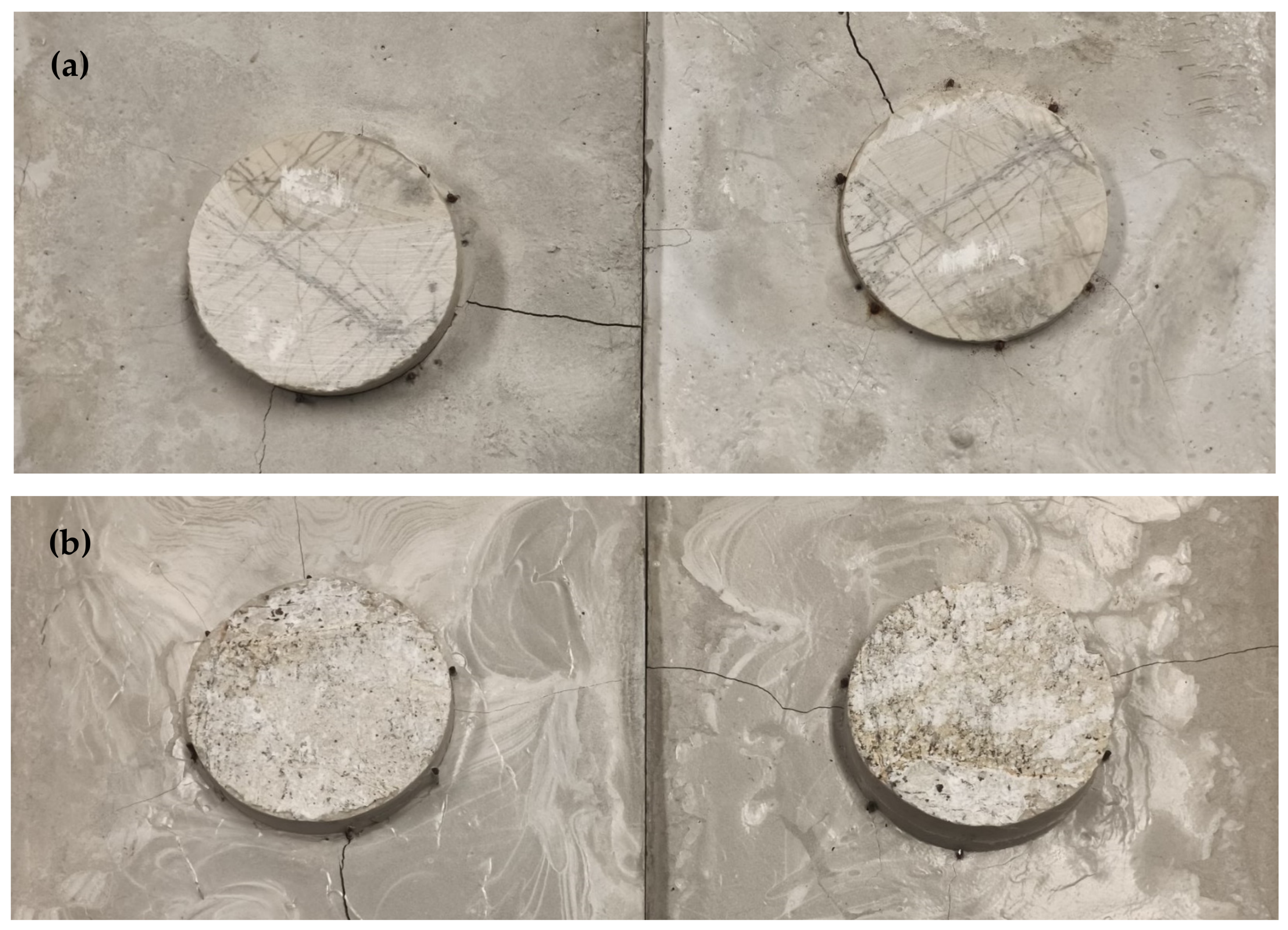
Artificial discontinuities were produced by sawing intact specimens in order to create smooth, planar shear surfaces with minimal roughness (Figure 7a), whereas natural discontinuities were tested without surface modification, preserving their original roughness (Figure 7b).

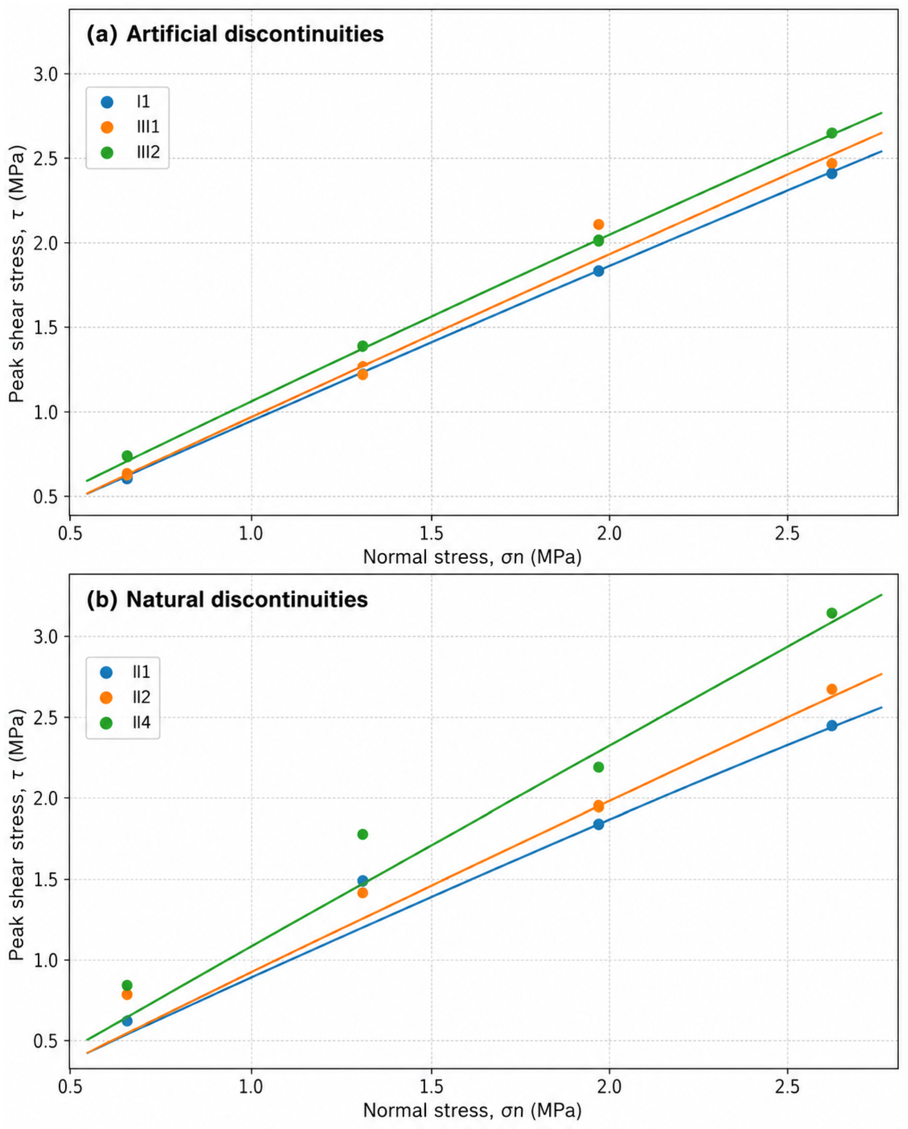
For the artificial saw-cut discontinuities, the following shear-strength envelopes were obtained (Figure 8a), with τ and σ_n expressed in MPa:

Specimen I-1: τ = 0.131 + 0.923σ_n, c = 131.0 kPa, φ = 42.7°, R² = 0.9770;

Specimen III-1: τ = 0.153 + 0.913σ_n, c = 152.8 kPa, φ = 42.4°, R² = 0.9773;

Specimen III-2: τ = 0.152 + 0.950σ_n, c = 152.0 kPa, φ = 43.5°, R² = 0.9999.

The relatively consistent friction angles, clustered around 42–44°, indicate that the shear resistance of the artificial discontinuities is primarily governed by the basic friction of the limestone surface, with limited contribution from roughness-induced mechanical interlocking.

For the natural discontinuities, the following shear-strength envelopes (Figure 8b) were obtained:

Specimen II-1: τ = 0.196 + 0.937σ_n, c = 196.5 kPa, φ = 43.1°, R² = 0.9539;

Specimen II-2: τ = 0.262 + 0.927σ_n, c = 262.0 kPa, φ = 42.8°, R² = 0.9993;

Specimen II-4: τ = 0.196 + 1.120σ_n, c = 196.5 kPa, φ = 48.2°, R² = 0.9766.

Compared with the artificial saw-cut surfaces, the natural discontinuities generally show higher apparent cohesion and, in specimen II-4, a higher friction angle. This difference reflects the contribution of surface roughness, asperity interlocking and natural joint morphology to the peak shear response.

The natural discontinuity specimens were selected to represent the accessible rough-joint conditions observed in the limestone rock mass. Although the number of natural joint specimens is limited, the use of four normal-stress levels for each specimen and the high coefficients of determination of the fitted envelopes provide a consistent estimate of peak shear-strength parameters for the tested surfaces. These parameters were not used to define explicit joint elements in the RS2 model, but to support the engineering-geological interpretation and the conservative definition of the weakened perimeter-zone properties.

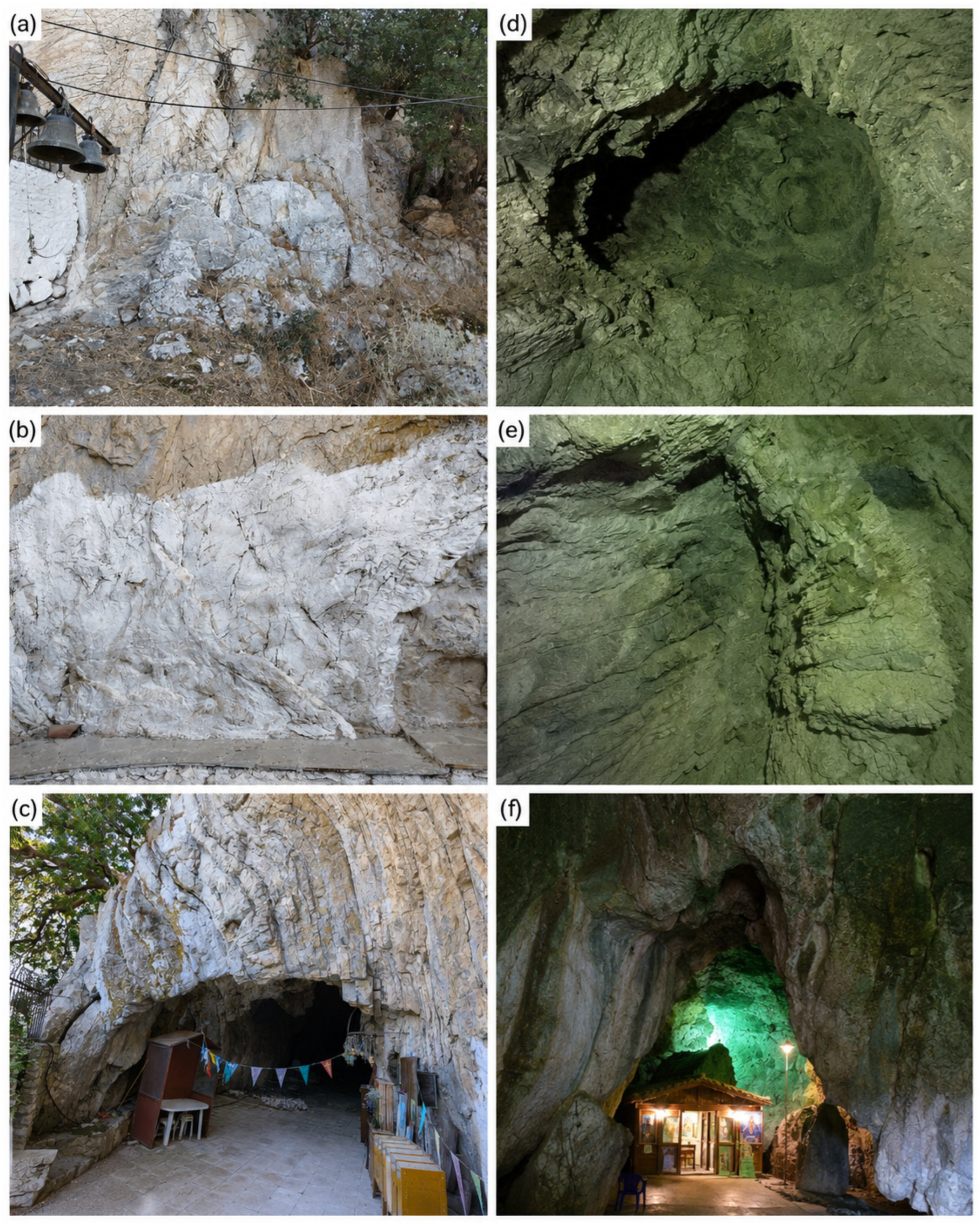
The photographic documentation of specimen II-1 reveals several important characteristics on the natural discontinuities of the tested rock mass:

• The shear surface is irregular and non-planar, exhibiting small-scale undulations and micro-asperities. The morphology corresponds to a moderately rough joint surface in ISRM terms.
• Post-shear inspection shows partial crushing and detachment of asperities along the sheared interface, especially near the specimen margins. This indicates brittle asperity failure, a mechanism commonly observed in limestone joints under direct shear.
• Visible vertical cracking in the specimen blocks suggests tensile stress redistribution during shearing. Such cracking is typical when normal stress is sufficient to mobilize dilation and induce local tensile stresses at asperity contacts.
• The joint surfaces appear clean, with no clay gouge or weathered filling material. Therefore, shear strength is dominated by rock-to-rock contact rather than frictional sliding over weak infill.
• No extensive smoothing or polishing is evident, implying that residual conditions were not fully mobilized within the displacement range applied.

These observations are consistent with the conceptual shear model for rough rock joints, where peak shear strength is controlled by a combination of basic friction and asperity interlocking, followed by progressive asperity degradation toward residual strength.

The comparison between artificial and natural discontinuities demonstrates that:

• Artificial joints provide an estimate of basic friction angle (φ) of the intact rock surface.
• Natural joints incorporate additional strength due to roughness, interlocking and micro-scale geometry.
• The difference in cohesion between artificial and natural surfaces reflects apparent cohesion generated by asperity interlocking rather than true cementation.

The artificial saw-cut discontinuity parameters were not considered to represent the current in-situ shear strength of the natural discontinuities in the cave rock mass. Instead, they were used as a conservative lower-bound reference for the weakened perimeter zone adopted in Scenario D. This interpretation assumes that progressive decompression, weathering, karstification and micro-fracturing along the cavity boundary may gradually reduce roughness-related strength and asperity interlocking. Therefore, the natural discontinuity tests were used to characterize the present rough-joint behaviour, whereas the smoother artificial surfaces provided a conservative reference for a degraded long-term boundary condition.

Overall, the results confirm that the limestone discontinuities exhibit high shear resistance, primarily controlled by frictional behaviour with secondary contribution from surface roughness, which is consistent with carbonate rock joint behaviour reported in the literature.

3.2. Rock Mass Discontinuity Analysis

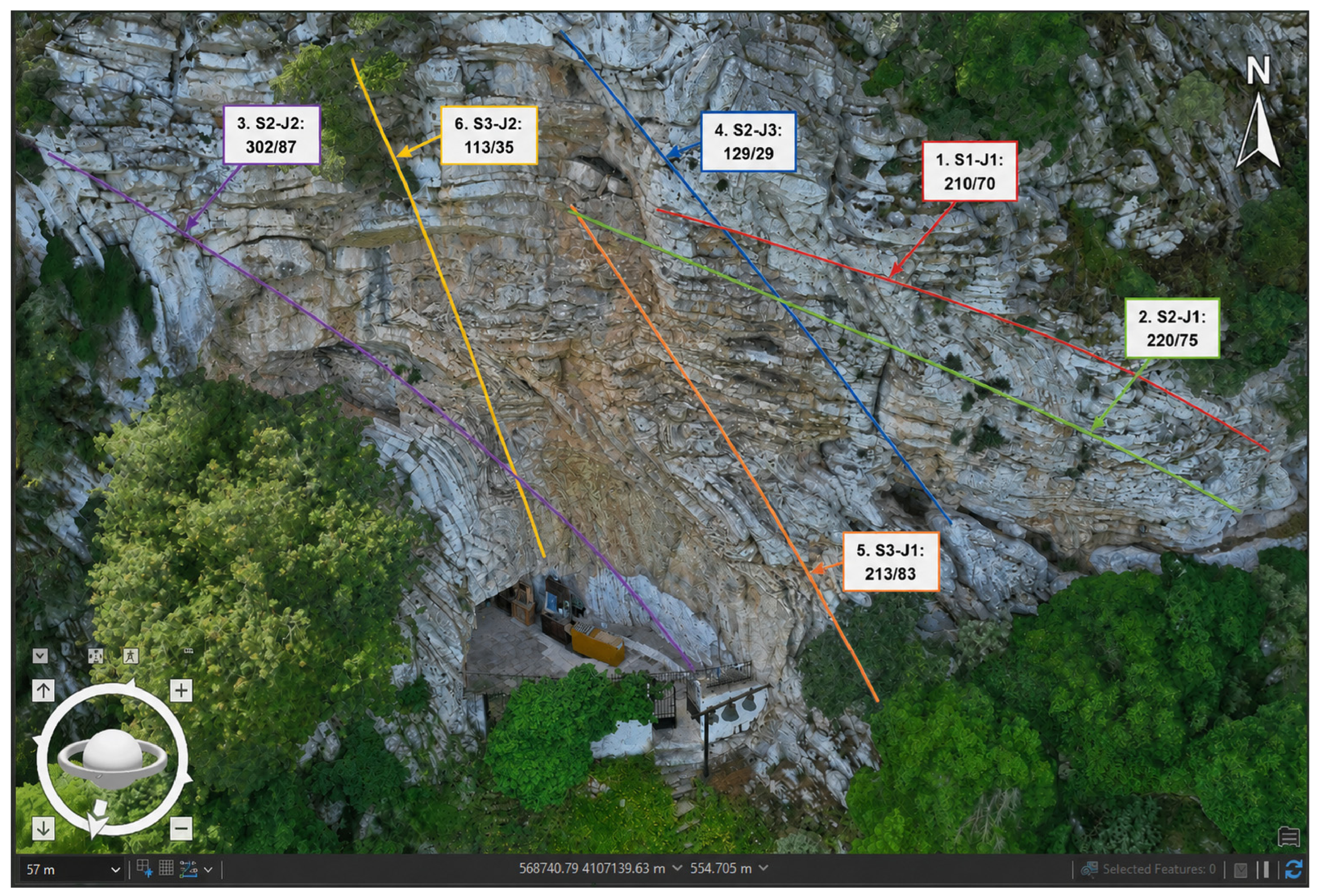
Discontinuity analysis was performed using an integrated approach that combines automated structural mapping from the UAV datasets with field-based documentation, in order to obtain reliable and spatially representative discontinuity sets for the host rock mass of the cave.

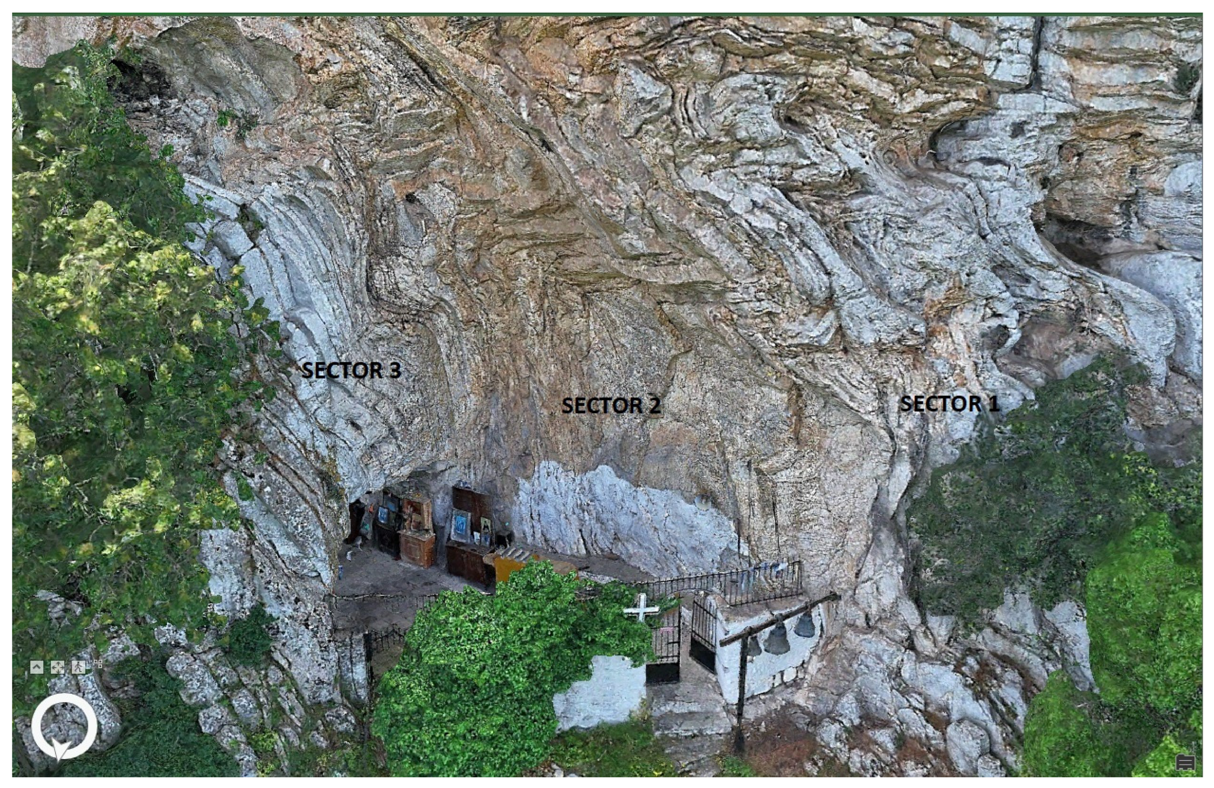
Specifically, discontinuity orientations measured in the field were imported into the Dips software version 9.029 [49], and the study area was subdivided into three sectors (Figure 2) to capture spatial variability and support the kinematic interpretation. The field dataset consisted of 97 discontinuity-orientation measurements in total. These were distributed across the three mapped sectors as follows: 32 measurements in Sector 1, 34 measurements in Sector 2, and 31 measurements in Sector 3. This sector-based subdivision was adopted to reduce spatial averaging and to allow direct comparison between field-measured Dips sets and DSE-extracted discontinuity sets within the same structural domains. Automated extraction of discontinuity sets was carried out on the UAV-derived point cloud dataset using the DSE software, initially for the entire surface and subsequently for three-point cloud subsets. These subsets were clipped in CloudCompare to match the DIPS sectors exactly, following the rationale of integrating field measurements with remote sensing data for rock mass structural mapping [50].

The Dips–DSE comparison was conducted for each sector using the orientation pairs expressed as dip direction/dip. The difference columns in

Table 3. Comparison between field-measured Dips discontinuity sets and DSE-extracted discontinuity sets. Differences are calculated as Dips − DSE.

Sector	Dips Set (DipDir/Dip)	DSE Set (DipDir/Dip)	ΔDipDir (°)= DipDirDips − DipDirDSE (°)	ΔDip (°)= DipDips − DipDSE (°)	Decision
1 Right of entrance	210/70	204/66	6	4	Retained
2 Entrance zone	220/75	210/55	10	20	Retained as corresponding trend; dip uncertainty noted
2 Entrance zone	302/87	311/88	9	1	Retained
2 Entrance zone	129/29				Retained from Dips
3 Left of entrance	213/83	207/68	6	15	Retained as corresponding trend; dip uncertainty noted
3 Left of entrance	113/35			—	Retained from Dips

were calculated as field-based Dips values minus DSE-extracted values, i.e., ΔDipDir = DipDir_Dips − DipDir_DSE and ΔDip = Dip_Dips − Dip_DSE. The comparison was used to identify corresponding structural trends rather than to imply exact one-to-one agreement between field and point-cloud-derived planes. DSE sets with relatively consistent dip directions were retained as representative digital structural trends, whereas field-measured low-dip discontinuities that were not clearly isolated by the automated extraction were retained from Dips because of their potential relevance to planar sliding and wedge geometry [51]. The final selection of discontinuity sets was then used as a consistent input basis for subsequent analyses, ensuring coherence between structural characterization, kinematic assessment, and numerical modelling, as recommended in recent integrated workflows for three-dimensional survey data and rock slope stability evaluation [17,36].

In Table 3, the discontinuity values derived using the Dips and DSE software are presented, along with their comparison.

Table 3 shows that the dominant steeply dipping discontinuity sets are generally consistent in terms of dip direction, with differences ranging from −9° to +10° for the matched Dips–DSE sets. However, the dip differences are not uniformly small. Differences of +20° in Sector 2 and +15° in Sector 3 indicate that the DSE-derived planes locally underestimate the dip angle relative to the field measurements. These discrepancies may be related to point-cloud resolution or shadow effects, local surface roughness, limited exposure of individual discontinuity planes, and the smoothing effect introduced when local normal vectors are calculated over irregular rock surfaces. Therefore, the Dips–DSE comparison should be interpreted as a structural-trend validation rather than as an exact match of individual discontinuity planes.

The orientation differences introduce uncertainty into the structural interpretation, especially for kinematic assessments where dip angle affects the identification of planar sliding or wedge-forming conditions. For this reason, the final discontinuity dataset was treated as a hybrid dataset: DSE results were used to support the recognition of the main exposed structural trends, while field measurements were retained where DSE did not clearly isolate low-dip or potentially critical discontinuities. This approach avoids over-reliance on automated extraction and provides a more conservative basis for subsequent rock mass characterization.

The discontinuity dataset was also used for a preliminary structural interpretation of potential kinematic conditions in the three mapped sectors. However, a full stereographic Markland analysis was not performed in the present study, because the numerical assessment was focused on an equivalent-continuum RS2 model rather than on explicit discontinuity-controlled failure mechanisms. Future work could combine the present UAV/DSE and field-measured discontinuity dataset with sector-specific slope face orientations and friction cones in a formal Markland-type kinematic analysis.

3.3. Rock Mass Quality

Rock mass quality was evaluated with RMR [22] and GSI [23,52] systems using the results from the UAV-Lidar rock mass characterization as well as the results from the discontinuity analysis and the lab tests.

The RMR system incorporates six parameters:

• Intact rock strength [53];
• Rock Quality Designation (RQD);
• Discontinuity spacing;
• Discontinuity condition;
• Groundwater conditions;
• Adjustment for discontinuity orientation.

The basic rating RMR_bas is derived from the first five parameters, while orientation correction is applied depending on the geometric relationship between discontinuities and the excavation [22].

The cave area was divided into three sectors (Figure 2) for independent evaluation, and results are presented in

Table 4. Sector-based rock mass categorization using RMR_bas and derived GSI values.

Sector	RMRbas	GSI (RMRbas − 5)
1	68	63
2	69	64
3	73	68

.

The GSI values were derived from the sector-based RMR_bas values using the empirical approximation GSI ≈ RMR_bas − 5 [23]. The RMR_bas ratings were based on field documentation of intact rock strength, discontinuity spacing, discontinuity condition and groundwater conditions. Discontinuity conditions were assessed using the recorded persistence, aperture, infilling, weathering and qualitative roughness observations collected during field mapping (Figure 9).

The resulting GSI values range between 63 and 68, corresponding to moderately fractured limestone with well-defined discontinuity sets and limited surface degradation. The results indicate that the rock mass ranges from fair to good quality. Differences between sectors are primarily controlled by discontinuity spacing and persistence rather than intact rock strength. Groundwater influence was negligible during field investigation and therefore did not significantly reduce the rating.

To derive equivalent rock mass strength parameters for numerical modelling, the generalized Hoek–Brown failure criterion [19,23] was adopted, in which the rock mass parameters are defined as:

$$m_b=m_{i}exp\left({\displaystyle \frac{GSI-100}{28-14D}}\right)$$

(1)

$$s=\exp \left({\displaystyle \frac{GSI-100}{9-3D}}\right)$$

(2)

$$a=0.5+{\displaystyle \frac{1}{6}}\left(e^{-GSI/15}-e^{-20/3}\right)$$

(3)

where m_b, s, and α are intact rock and rock mass constants; m_i is a laboratory determined intact rock constant; and D is the disturbance factor.

For limestone of the type encountered in the study area, a representative value of mi = 10 was adopted based on published ranges for carbonate rocks. Since the cave represents a natural cavity without blasting-induced damage, a disturbance factor D = 0 was considered appropriate.

The resulting Hoek–Brown parameters used in the numerical modelling and the stability analysis are summarized in

Table 5. Calculation of the Hoek–Brown parameters used in numerical modelling.

Sector	GSI	mb	s	a
1	63	2.67	0.016	0.502
2	64	2.76	0.018	0.502
3	68	3.19	0.029	0.502

.

The transformation from RMR to GSI and subsequently to the Hoek–Brown parameters provide a consistent framework for incorporating field and laboratory data into numerical modelling. While the intact limestone exhibits relatively high compressive strength, the mechanical behaviour of the system is governed by discontinuity structure and rock mass quality.

The derived Hoek–Brown parameters were used as input in the finite element model to represent equivalent rock mass strength. This approach ensures that the numerical simulation reflects realistic large-scale behaviour rather than intact rock properties alone.

3.4. Elasto-Plastic Finite Element Analysis

The stability of the rock slope and the natural cavity was investigated using the finite element method in RS2 Rocscience [21]. The analyses were performed under plane strain conditions, with the geometry discretized into triangular finite elements. The rock mass was modelled as an elastic–plastic continuum governed by the Hoek–Brown failure criterion, which is widely adopted for jointed rock masses and incorporates the influence of rock mass quality through the parameters m_b, s and the uniaxial compressive strength.

Initial stresses were generated through gravity loading combined with a horizontal-to-vertical effective stress ratio. Boundary conditions consisted of zero horizontal displacement along the lateral boundaries and zero vertical displacement at the base of the model. Stability was assessed using the Shear Strength Reduction method. In this approach, the shear strength parameters are progressively reduced by a factor F until numerical non-convergence or generalized plastic yielding occurs. The value of F at failure corresponds to the Strength Reduction Factor, which is interpreted as an equivalent factor of safety [20]. The input parameters and modelling settings used in the current elasto-plastic finite element analysis for all scenarios executed are presented in

Table 6. RS2 input parameters and modelling settings used in the finite element analyses.

Parameter	Value/Setting Used in RS2
Deformation assumption	Plane strain
Material model	Generalized Hoek–Brown equivalent continuum
Elastic model	Linear elastic
Stability method	Shear Strength Reduction (SSR)
Solver	Initial stiffness method; Gauss elimination
Number of stages	2
Stage 1	Geostatic stage
Stage 2	Excavation stage
Model dimensions	82.66 m wide × 66.01 m high
Cavity extent in selected section	x = 33.64 to 43.47 m; y = 554.55 to 566.95 m
Approximate boundary distance from cavity	Left: ~33.6 m; right: ~39.2 m; lower boundary below cavity: ~29.6 m; upper boundary above cavity: ~24.0 m
Boundary conditions	External model boundaries restrained; excavation/cavity boundary free after excavation stage
Initial stress condition	Gravity loading
Horizontal-to-vertical stress ratio, K0	0.45
Groundwater condition	No groundwater pressure applied; dry condition assumed
Convergence tolerance	0.001
Maximum iterations	500
SSR tolerance	0.001
SSR factor increment control	ΔFS = 0.01
Mesh type, Scenarios A–C	Quadratic triangular finite elements
Mesh, Scenarios A–C	4014 elements; 8299 nodes
Mesh type, Scenario D	Quadratic triangular finite elements with local refinement around the material boundary
Mesh, Scenario D	7740 elements; 15,755 nodes
Rock mass classification basis	Sector-based RMR–GSI assessment: RMRbas = 68–73 and GSI = 63–68. These values were used to support the selection of equivalent rock mass parameters
Rock mass, Scenario A	Reference static condition, gravity loading only: γ = 27.35 kN/m3; E = 15.8 GPa; ν = 0.30; UCS = 60.9 MPa; mb = 1.862; s = 0.001148; a = 0.50
Rock mass, Scenario B	Degraded rock mass condition: γ = 27.35 kN/m3; E = 8 GPa; ν = 0.30; UCS = 70 MPa; mb = 1.73; s = 0.0057; a = 0.50
Rock mass, Scenario C	Same rock mass parameters as Scenario A, with pseudo-static horizontal seismic coefficient kh = 0.15 applied in the unfavourable horizontal direction; the negative sign denotes the selected direction of horizontal inertial loading
Scenario D background rock mass	Same degraded background material as Scenario B
Scenario D with a weakened perimeter zone	γ = 25.23 kN/m3; E = 6 GPa; ν = 0.20; UCS = 40 MPa; mb = 0.80; s = 0.0015; a = 0.50
Thickness of weakened perimeter zone	Variable with an average value of about 1.3 m
Basis for Scenario D weakened zone	Field evidence of disturbed, decompressed, weathered, karstified and locally loosened rock around the cavity perimeter

.

Although the mapped discontinuity data were used to support the engineering-geological interpretation, sector-based rock mass characterization, RMR–GSI assessment and definition of equivalent rock mass parameters, the discontinuity sets were not introduced into RS2 as discrete joints, interface elements, ubiquitous joint sets or explicit discontinuum blocks. Instead, their influence was incorporated indirectly through the equivalent-continuum Hoek–Brown rock mass parameters and through the interpretation of the structurally controlled sectors. The numerical model should therefore be interpreted as an equivalent-continuum finite element assessment of the selected cavity–slope section, rather than as a discontinuum simulation of individual block release, wedge detachment or structurally controlled failure along explicitly modelled joints. Accordingly, the plasticity patterns and SRF values obtained from the FEM analyses are interpreted as indicators of the overall equivalent-continuum response of the selected cavity–slope section and not as direct simulations of structurally controlled block detachment or discontinuity-guided failure mechanisms.

This modelling approach has inherent limitations, as it depends on the software used for the later finite element analysis. Although the UAV–LiDAR survey captures the three-dimensional geometry of the external slope, cave entrance and internal cavity, the RS2 analysis used in this study represents only the selected Section 2–2 under plane-strain conditions. Consequently, the model evaluates the equivalent continuum response of this representative section and does not explicitly reproduce three-dimensional wedge release, individual block detachment, or spatially variable discontinuity persistence. The results should therefore be interpreted as a scenario-based assessment of the overall mechanical response of the selected cavity–slope section.

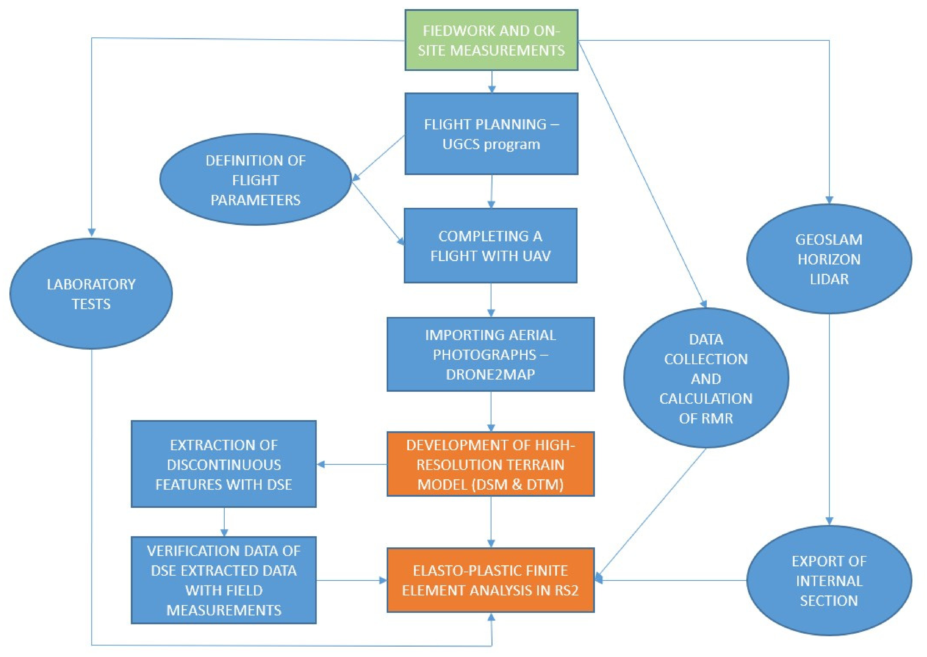
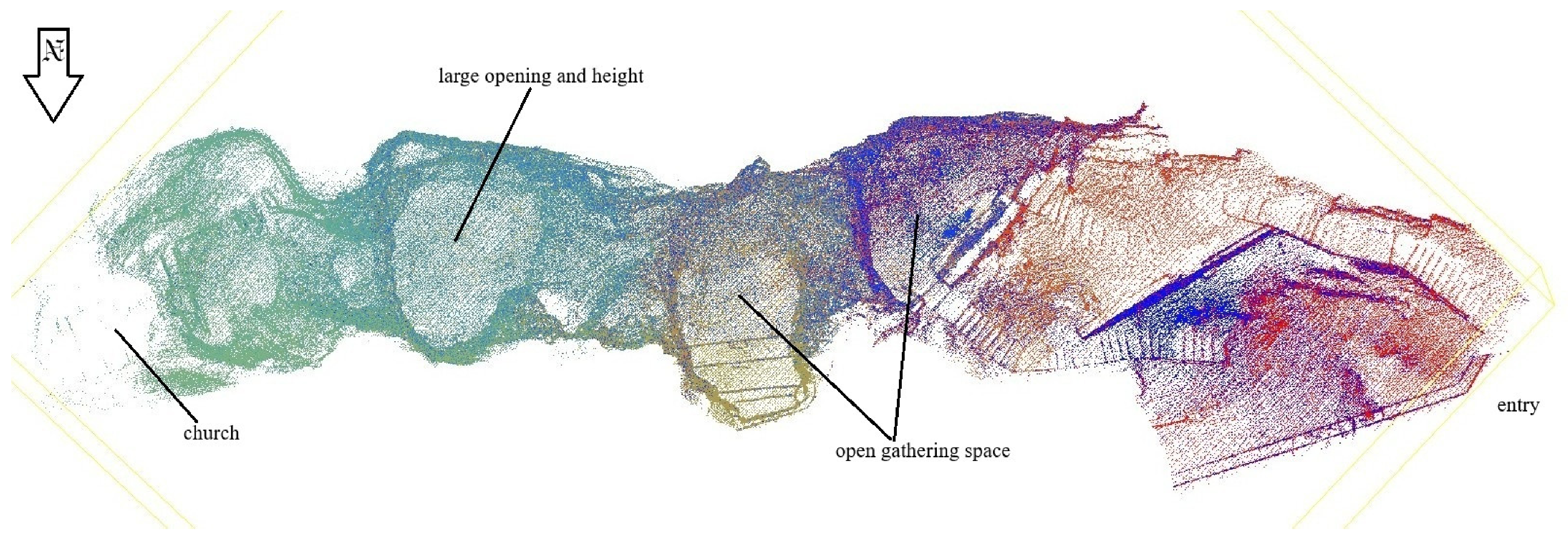
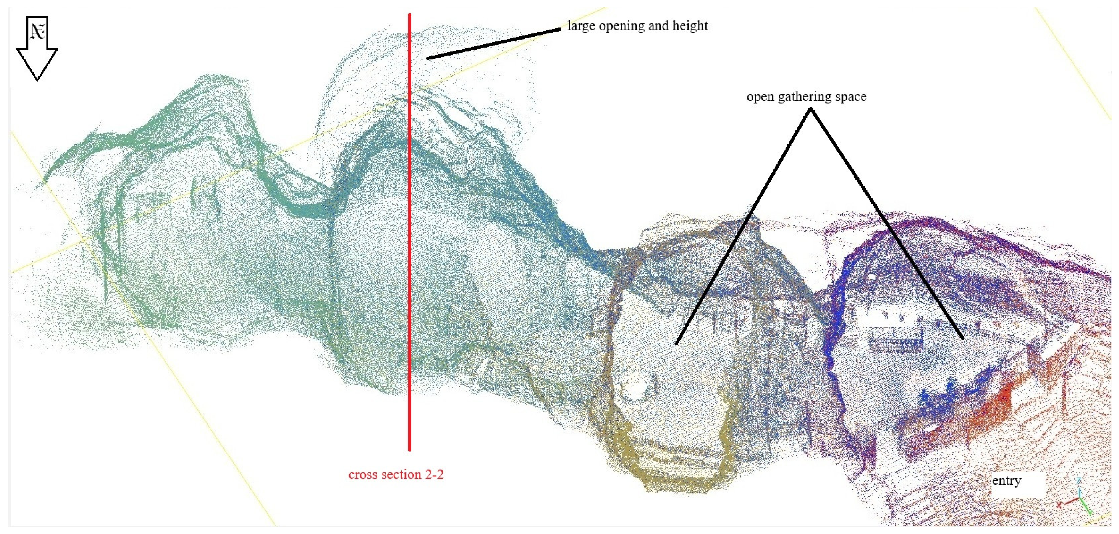
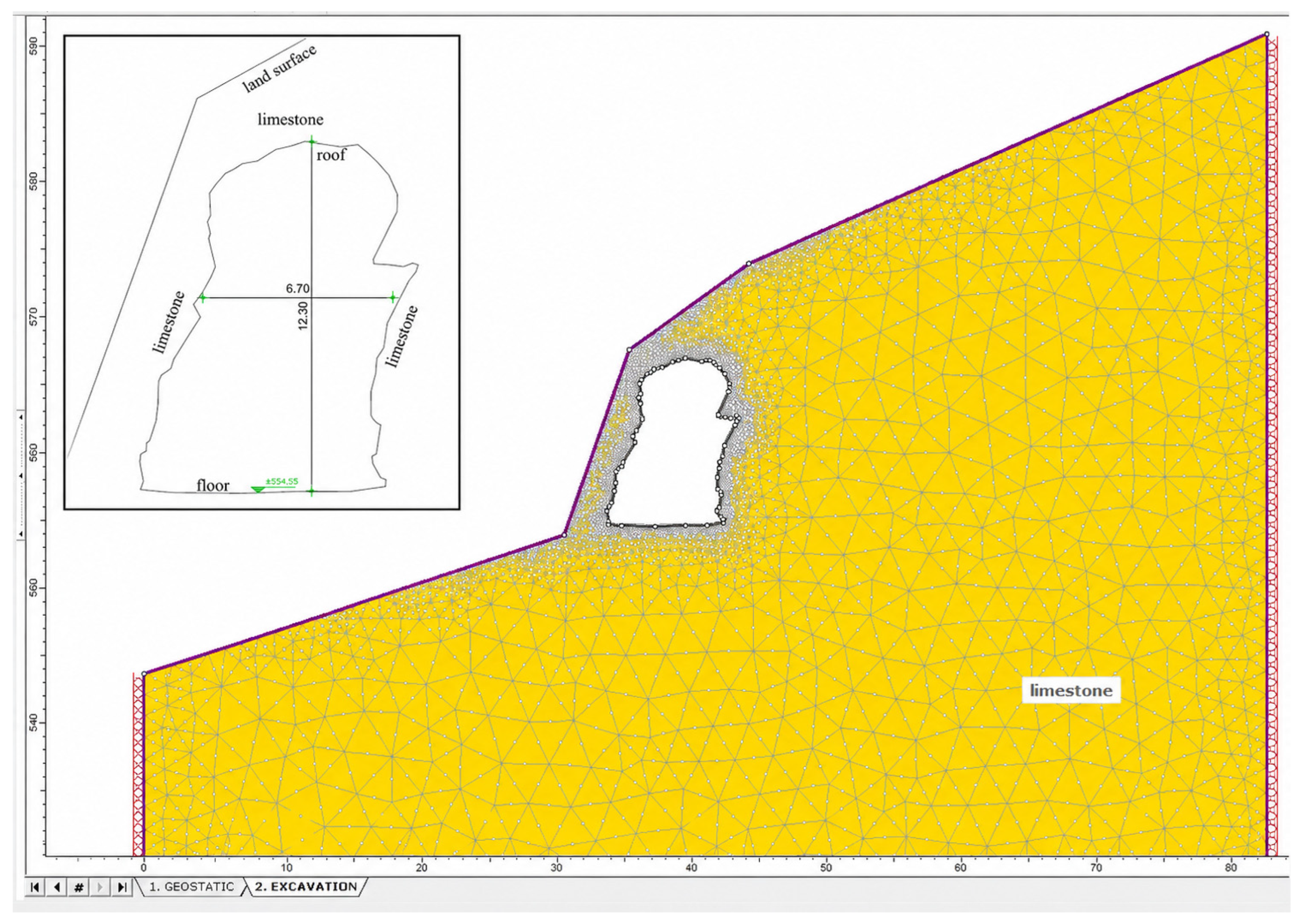
Figure 10 presents the two-dimensional cross-section used for the numerical simulation in RS2. The section was generated by combining the external cave morphology, derived from UAV photogrammetric surveying and Drone2Map processing, with the internal cave geometry along Section 2–2, which was acquired through terrestrial LiDAR scanning. This integrated approach allowed a more geometrically complete and consistent representation of the relationship between the external surface of the rock slope and the internal cave void, providing a suitable basis for the implementation of the stability scenarios in RS2.

Four scenarios were examined to evaluate the influence of mechanical degradation, seismic loading and the presence of a disturbed zone around the cavity in terms of SRF (Strength Reduction Factor). SRF is the factor used in the Shear Strength Reduction method to progressively reduce the shear strength parameters of the rock mass or soil material. During the analysis, the material strength gradually decreased until the numerical model reaches failure or no longer converges. The SRF value at this critical state is commonly interpreted as the factor of safety of the slope or underground opening. Higher SRF values indicate a greater stability margin, whereas values close to or lower than 1 suggest marginal or unacceptable stability.

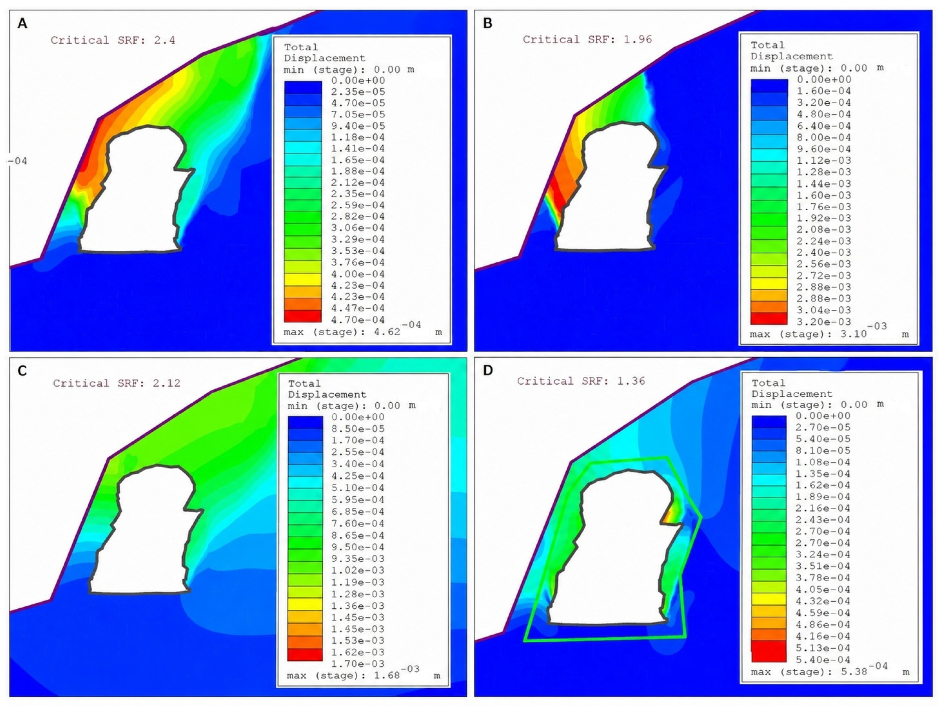
Scenario A represents the reference condition. It includes the original slope geometry, the estimated mechanical parameters of the limestone rock mass and gravity loading only. The computed Critical SRF was 2.40. Maximum total displacements were on the order of 4.62 × 10⁻⁴ m, while maximum shear strains were approximately 6.53 × 10⁻⁴. Plastic zones were localized mainly at the toe of the slope and around the cavity perimeter, without evidence of global slope failure. This scenario indicates a significant stability margin under static conditions.

Scenario B was designed to investigate the response of the cavity–slope system under a modified, less favourable rock mass parameter set. In this scenario, the rock mass deformation modulus was reduced from 15.8 GPa to 8 GPa. In addition, Scenario B was not limited to a stiffness-only modification; a separate Hoek–Brown parameter set was also assigned, as reported in Table 6. The Critical SRF decreased from 2.40 in Scenario A to 1.96 in Scenario B. This reduction is therefore interpreted as the result of the combined modified mechanical parameter set used in Scenario B, rather than as the effect of Young’s modulus reduction alone.

Scenario C retains the mechanical parameters of Scenario A and introduces pseudo-static seismic loading. A horizontal seismic coefficient k_h = 0.15 was applied in the unfavourable horizontal direction. In RS2, k_h is a dimensionless pseudo-static coefficient that represents a horizontal inertial acceleration equal to k_h·g; therefore, k_h = 0.15 corresponds to a horizontal acceleration equal to 15% of gravity. The value was selected as a sensitivity coefficient informed by the regional seismic hazard, rather than as a full code-based dynamic seismic analysis. According to the Greek seismic zonation of the Hellenic Seismic Code, the wider study area belongs to Seismic Hazard Zone II, for which the reference design ground acceleration is a = 0.24 g [54]. A commonly adopted pseudo-static approximation based on one-half of this reference acceleration gives k_h ≈ 0.5 a/g = 0.12. The value adopted in this study, k_h = 0.15, is therefore slightly higher than this simplified reference value and is used to examine the response of the selected cavity–slope section under adverse horizontal inertial loading. The Critical SRF was calculated as 2.12. Maximum total displacement reached 1.68 × 10⁻³ m, while maximum shear strain was approximately 4.10 × 10⁻⁴. Plastic zones developed mainly around the cavity perimeter and within the slope, but without indication of global instability. Compared with the static reference case, this pseudo-static loading reduced the stability margin; however, for the adopted sensitivity coefficient, the system remained stable with SRF greater than unity.

Scenario D represents the governing long-term geological evolution scenario of the cave–slope system. In contrast to the previous scenarios, which mainly examine the influence of global rock mass degradation and pseudo-static seismic loading, this scenario explicitly introduces a weakened perimeter zone around the cavity. This zone was used to represent the progressive decompression, weathering, and micro-fracturing that commonly develop along the boundary of natural limestone cavities during their long-term evolution. As a result, this scenario should not be interpreted as a simulation of a sudden large-scale continuum collapse of the cave or progressive failure of large rock blocks. Instead, it represents an equivalent-continuum approximation of progressive degradation processes along the cavity boundary, which are commonly controlled by discontinuity conditions, loss of asperity interlocking and long-term weathering. At the time of the field investigation, at the time of the field investigation, no clear evidence of recent fallen blocks on the cave floor was documented to support an active large-block collapse mechanism.

The reduced mechanical properties assigned to this zone were justified by combining field-based rock mass characterization with the conservative interpretation of the direct shear tests. In particular, the lower-bound shear strength parameters derived from the smoother artificial discontinuities were adopted to represent a degraded long-term condition, where roughness interlocking and local asperity contribution may be progressively reduced. This does not imply that the geomechanical role of natural discontinuities was ignored. The natural discontinuity tests were used to characterize the present rough-joint peak behaviour of the rock mass, whereas the artificial saw-cut results were used only to define a conservative lower-bound condition for a possible degraded long-term state of the cavity perimeter. This use of the artificial-discontinuity results should therefore be interpreted only as a conservative lower-bound assumption for a degraded boundary zone, and not as a direct representation of the current peak strength of the natural discontinuity network.

The thickness of the weakened perimeter zone was defined from the LiDAR-derived cavity boundary and field observations of disturbed rock around the cave perimeter, whereas its reduced strength was assigned as a conservative lower-bound condition informed by the smoother artificial direct shear results. This interpretation is consistent with rough-joint shear-strength concepts, in which degradation of surface roughness and asperity interlocking reduces peak shear resistance [34], and with finite-element approaches that represent thin weak layers as lower-strength zones [55].

The results, summarized in

Table 7. Aggregated analysis results of A, B, C, and D Scenarios executed with the program RS2.

Scenario	Description	Critical SRF	Maximum Displacement (m)	Maximum Shear Strain, γmax
A	Baseline static condition	2.40	4.62 × 10−4	6.53 × 10−4
B	Modified/degraded rock mass parameter set	1.96	3.10 × 10−3	4.17 × 10−3
C	Baseline with seismic loading	2.12	1.68 × 10−3	4.10 × 10−4
D	Weakened zone around the cavity	1.36	5.38 × 10−4	8.55 × 10−4

and presented in Figure 11 as total displacement around the cavity, show the relative response of the selected cavity–slope section under different material and loading assumptions. Because the external slope geometry was kept unchanged in all four analyses, the comparison should be interpreted as a scenario-based assessment of the influence of rock mass condition, pseudo-static loading and cavity-perimeter weakening for the fixed geometry analysed.

The comparison of the four scenarios indicates that, for the fixed section and geometry analysed, the weakest response was obtained when a weakened perimeter zone was introduced around the cavity. The baseline model indicates a substantial stability margin, whereas pseudo-static seismic loading and generalized degradation of the rock mass reduce the SRF without producing critical instability. Scenario D produced the lowest Critical SRF, equal to 1.36, and concentrated plastic yielding around the cavity boundary. This result suggests that, within the adopted equivalent-continuum model and for the selected cavity–slope section, local degradation around the cave perimeter has a strong influence on the computed stability margin. However, the comparison does not prove that internal geotechnical conditions generally govern stability more strongly than external slope morphology, since the slope geometry was not varied between scenarios. Scenario D is therefore interpreted as the most critical case among the examined scenarios for the specific geometry analysed.

The spatial pattern of the computed plastic zones was also compared qualitatively with the engineering-geological observations made during field investigation. In Scenario D, plastic yielding was mainly concentrated around the cavity perimeter, which is consistent with the observed disturbed rock mass zone along the cave boundary. This comparison is qualitative, because no displacement monitoring data or detailed post-failure inventory are available for the site. Therefore, field observations are used only as a plausibility check of the computed deformation pattern and not as an independent validation of the numerical results.

4. Discussion

The present study demonstrates the development and implementation of a unified multi-scale spatial data fusion framework for the quantitative assessment of rock mass stability in natural cavities and large underground openings. The proposed workflow combines external UAV photogrammetric reconstruction, internal SLAM-based LiDAR mapping, discontinuity analysis, laboratory testing, rock mass classification and finite element analysis. This integration is particularly important in natural cave environments, where stability is controlled by the combined effect of external slope morphology, internal void geometry, discontinuity patterns and local rock mass degradation. The main methodological contribution is therefore the integration of established survey, laboratory and numerical techniques into a single cavity–slope assessment workflow.

UAV photogrammetry provided a detailed representation of the external limestone slope and supported the extraction of structural information from the exposed rock mass. In parallel, SLAM-based LiDAR scanning captured the internal cave geometry, including the roof, sidewalls and areas that could not be reliably documented by aerial photogrammetry alone. The integration of these datasets improved the geometric reliability of the model and enabled the construction of a representative cross-section through the largest cave opening. Similar advantages of photogrammetric and LiDAR-based approaches for rock mass characterization and stability assessment in other works have also been reported [26,35,50,56].

In this work it should be clarified that the structural interpretation is based mainly on external field measurements and UAV/DSE-derived discontinuity extraction. The internal SLAM LiDAR survey was used to define the cave geometry and to support the extraction of the numerical cross-section, but it was not used to derive a separate internal discontinuity-set population. Any structural relationship between the external and internal domains is treated as an engineering-geological interpretation of the coupled cavity–slope system, rather than as a quantitatively demonstrated discontinuity–continuity model.

The comparison between DSE-based 3D discontinuity extraction and Dips software from field measurements showed that the dominant steeply dipping discontinuity sets were consistently identified, especially after subdividing the UAV-derived point cloud into sectors corresponding to the field mapping domains. This sector-based approach reduced spatial averaging and improved the structural representativeness of the dataset. However, low-dip discontinuities were not always clearly detected by the automated extraction and were therefore retained from field observations. This confirms that UAV-based structural mapping should be used as a complementary tool to conventional field mapping, rather than as a replacement for it.

It should also be noted that the mapped discontinuity sets were used to constrain the structural interpretation and rock mass characterization, but they were not explicitly represented in the RS2 model. Therefore, the computed plastic zones should not be interpreted as predicted discontinuity-controlled failure surfaces. Instead, they indicate zones where the equivalent continuum reaches plastic yielding under the adopted material parameters and loading assumptions. Potential structurally controlled mechanisms, such as block detachment, wedge release or sliding along persistent joints, would require a discontinuum or explicitly jointed modelling approach and are outside the scope of the present RS2 analysis.

The laboratory direct shear tests and rock mass classification results provided the geomechanical basis for the numerical analysis. The shear tests indicated relatively high shear resistance of the limestone discontinuities, mainly controlled by frictional behaviour and secondarily influenced by surface roughness, in agreement with classical rock joint shear behaviour. RMR and GSI systems were then used to translate field observations, discontinuity conditions and laboratory-derived parameters into representative rock mass properties for Hoek–Brown-based numerical modelling [22,23,52].

Another primary contribution of this work lies in quantifying the mechanical behavior of the highly complex, coupled cavity-slope system under long-term rock mass degradation using finite element analyses on a 2D model accurately reproduced by the previous multi-scale spatial data driven approach. While standard numerical simulations treat underground openings as idealized, sharp boundaries within a uniform continuum, the finite element Scenario D introduces an empirically calibrated, weakened decompressed ring surrounding the cavity perimeter. Within the fixed geometry analysed, Scenario D produced a distinct concentration of plastic yielding around the weakened cavity perimeter and the lowest Critical SRF among the examined scenarios. This response suggests that local degradation of the cave boundary may substantially reduce the computed stability margin of the selected cavity–slope section. However, because the external slope morphology was not varied between scenarios, the results should not be interpreted as proving that internal geotechnical conditions generally dominate over slope geometry. Instead, they indicate that, for the analysed section, the inclusion of a weakened cavity-perimeter zone is critical for obtaining a conservative assessment of long-term stability. For the fixed section and geometry analysed, the results indicate that the degraded cavity-perimeter zone produced the most critical response among the scenarios examined.

It should be emphasized that the four numerical cases presented in this study constitute a scenario-based comparison rather than a full parametric sensitivity analysis. A broader sensitivity analysis would require systematic variation in several parameters, including GSI, Hoek–Brown parameters, deformation modulus, UCS, K₀, pseudo-static seismic coefficient, groundwater conditions, weakened-zone thickness and weakened-zone strength. Such an analysis would substantially expand the numerical scope of the study and would require additional independently constrained parameter ranges, which are not available for the present case study. Consequently, the numerical conclusions are limited to the selected Section 2–2, the fixed geometry analysed and the adopted scenario-specific parameter sets. The results should therefore be interpreted as identifying the most critical response among the scenarios examined, and not as a complete sensitivity ranking of all possible controlling parameters.

Overall, the main contribution of the study is not limited to the calculation of critical SRF values but lies in the development of a reproducible workflow that links UAV–LiDAR survey data, field measurements, laboratory testing and numerical modelling. This integrated methodology improves geometric completeness and consistency, strengthens rock mass characterization and supports a more transparent quantitative stability assessment of natural caves and large underground cavities developed in fractured carbonate rock masses.

5. Conclusions

This study developed and applied an integrated UAV–LiDAR-based methodology for the quantitative assessment of rock mass stability in a natural cave environment. The workflow combined UAV photogrammetry, SLAM-based LiDAR scanning, field discontinuity mapping, laboratory testing, rock mass classification and finite element analysis.

The integration of UAV and LiDAR data allowed the external slope morphology and the internal cave geometry to be represented within a consistent geometric framework. This improved the reliability of the numerical cross-section and reduced the uncertainty associated with simplified geometric assumptions.

The comparison between automated discontinuity extraction and field measurements showed that UAV-derived point clouds can effectively support rock mass characterization, especially for clearly exposed and steeply dipping discontinuity sets. Nevertheless, field mapping remains necessary for identifying structurally important features that may not be fully captured by automated extraction.

Laboratory testing and RMR–GSI classification provided the basis for assigning representative mechanical parameters to the numerical model. This ensured that the finite element simulations reflected the overall behaviour of the limestone rock mass rather than only intact rock properties or isolated discontinuity strength values.

The numerical scenarios showed that, for the fixed section and geometry analysed, the lowest SRF was obtained when a weakened zone was introduced around the cave perimeter. This indicates that local degradation of the cavity boundary can substantially influence the computed stability margin and should be considered explicitly in long-term assessments of natural limestone cavities. The lowest SRF was obtained when a weakened zone was introduced around the cave perimeter, while pseudo-static seismic loading produced a secondary but still significant reduction in stability.

It should also be noted that the numerical analysis was performed using a two-dimensional equivalent-continuum finite element model. Consequently, the computed SRF values and plastic zones describe the overall response of the selected cavity–slope section under the adopted Hoek–Brown parameters and scenario assumptions. The model does not explicitly simulate discontinuity-controlled mechanisms such as three-dimensional wedge release, individual block detachment, sliding along persistent joints or spatial variability of joint persistence. Such mechanisms would require a discontinuum or explicitly jointed modelling approach.

In conclusion, the proposed methodology provides a robust and transferable framework for the stability assessment of natural caves and large underground cavities. By integrating high-resolution geomatic data with geomechanical characterization and numerical modelling, it supports a more reliable evaluation of complex fractured carbonate rock masses.