Article

Subducting Slab—Upper Plate Configuration, and Three-Dimensional Thermal Structure of Central-Southern Peru

1
Istituto Nazionale di Geofisica e Vulcanologia, Via di Vigna Murata 605, 00143 Rome, Italy
2
Sezione di Geologia, Scuola di Scienze e Tecnologie, Università degli Studi di Camerino, Via Gentile III da Varano 7, 62032 Camerino, Italy
3
Dipartimento di Scienze Pure e Applicate (DiSPeA), Università di Urbino “Carlo Bo”, Via Aurelio Saffi 2, 61029 Urbino, Italy
*
Author to whom correspondence should be addressed.
Geosciences 2026, 16(6), 216; https://doi.org/10.3390/geosciences16060216 (registering DOI)
Submission received: 3 April 2026 / Revised: 15 May 2026 / Accepted: 27 May 2026 / Published: 30 May 2026

Abstract

The study investigates the three-dimensional architecture and thermal structure of the Central Andes in centralsouthern Peru, highlighting the interplay between basement structure, Moho geometry, slab configuration, and thermal properties. Basement structural highs and lows acted as zones of weakness that localized deformation during Andean shortening. The Moho exhibits significant lateral heterogeneity, reflecting the combined effects of subduction processes, crustal shortening, magmatic underplating, and lower crustal flow or delamination. Its geometry provides key constraints on crustal thickness, seismic structure, and lithospheric dynamics. The subducting Nazca Plate shows strong along-strike variations in dip and continuity, influenced by plate kinematics and features such as the Nazca Ridge. These variations control mantle wedge development, arc magmatism, and deformation patterns in the overriding plate, contributing to the segmentation of the Andes. Steepslab segments promote mantle melting and volcanic activity, whereas flat-slab regions suppress magmatism. Consistent with these tectonic controls, Qs values increase from northwest to southeast, reflecting a transition from flat-slab conditions with low heat flow and limited geothermal activity to steep subduction zones characterized by active magmatism, elevated heat flow, and significant geothermal potential. This spatial variation underscores the strong coupling between slab geometry, thermal structure, and surface geothermal expression.

1. Introduction

Many Earth processes result in changes in the thermal structure and surface heat flow over large regions (e.g., Ranalli, 1995 [1]). Understanding the thermal structure of a region, in turn, is relevant for a series of applications, including, e.g., geothermal exploration and subsurface gas storage/waste disposal, as well as seismotectonic studies in active tectonic settings. Investigating the thermal structure of the crust may be carried out using various methodologies, which provide fundamental constraints on the thermo-tectonic setting of the region of interest (e.g., McKenzie et al., 2005 [2]). In oceanic environments, the cooling history of oceanic lithosphere is, to a first approximation, well described by classical cooling models and stands as one of the most robustly understood aspects of plate tectonics (e.g., Grose et al., 2013 [3]). In contrast, for stable and ancient continental regions (cratons), assuming thermal steady state is generally a valid simplification (e.g., Morgan et al., 1984 [4]). On the other hand, orogenic belts located at active plate margins—such as those formed at subduction zones and continental collision zones—show strong spatial and temporal variations in temperature (e.g., Royden, 1993 [5]). Classic studies (e.g., Brown, 1993 [6], and references therein) illustrated how these belts are characterized by a highly heterogeneous thermal structure that reflects the dynamic interplay of plate convergence, crustal thickening, magmatism, and fluid circulation. In contrast to stable cratonic regions, these belts exhibit pronounced lateral and vertical variations in geothermal gradients, resulting from the coexistence of relatively cold and hot domains within the same tectonic system. The same classic studies also pointed out that the descending oceanic lithosphere at subduction zones remains comparatively cold as it penetrates into the mantle, generating high-pressure metamorphic conditions that are achieved along normal cold subduction-zone geotherms (Syracuse et al., 2010 [7]) and are typically recorded by blueschist- and eclogite-facies assemblages (the blueschist facies representing either a prograde metamorphic stage preceding eclogitization or a retrograde overprint during exhumation). Geothermal gradients in these environments may be as low as 5–10 °C/km. Above the relatively cold subducting slab, the mantle wedge is thermally heterogeneous, consisting of a partially refrigerated mantle wedge immediately overlying the slab, and a hotter, convecting asthenospheric mantle wedge located between the refrigerated wedge and the overriding plate. Heat within the system is supplied primarily by mantle advection (corner flow) and conduction. Fluids released during slab dehydration hydrate the mantle wedge and lower the solidus, thereby promoting partial melting and the development of volcanic arcs. Arc magmatism and shallow crustal intrusions contribute to elevated temperature conditions in the overlying upper crust. Lithospheric-scale heat transport within active orogenic systems is dominated by conduction and large-scale advection. In particular, mantle heat transport occurs by advection associated with flow. On the other hand, conductive heat transfer dominates in thickened crustal domains, whereas advective processes, including the rising of magma and deforming crustal material, play a crucial role in redistributing heat, particularly in subduction-related environments. Additionally, hydrothermal fluid circulation can locally enhance heat transfer and modify the thermal structure of the upper crust. The thermal architecture of subduction-related mountain belts in general evolves through time, typically transitioning from an initially cold geotherm associated with active subduction to progressively warmer conditions during crustal thickening and eventual thermal relaxation. This evolution exerts a fundamental control on metamorphic processes, leading to the development of distinct pressure–temperature regimes that are diagnostic of specific tectonic settings, including high-pressure assemblages in the subducting slab (in cold, normal subduction zones with low geothermal gradients), intermediate thermal regimes in regional metamorphism affecting the overriding plate (where high-temperature metamorphic assemblages, e.g., amphibolite- and granulite-facies, may develop, particularly in regions of crustal thickening or magmatic underplating), and low-pressure/high-temperature conditions in extensional or back-arc environments. In these contexts, geotherms can be derived from surface heat-flow measurements combined with knowledge of thermal conductivity and the distribution of radiogenic heat sources (e.g., Furlong and Chapman, 2013 [8], and references therein). However, since the distribution of radiogenic elements within the crust remains uncertain, large-scale insights into crustal temperatures rely heavily on geophysical observations and on thermal modelling. The latter plays a particularly critical role in understanding the thermal structure of the continental crust, particularly in orogenic belts, where structural complexity and lateral heterogeneity are far greater than in oceanic domains. In these settings, realistic representations require three-dimensional models that explicitly incorporate internal heat production from radiogenic elements within the crust, as well as its spatial variability. In this study, we integrate subsurface geology and deep geophysical constraints with thermal modelling to investigate the effects of slab geometry and ridge subduction, with the aim of obtaining a better understanding of the geodynamic evolution of one of the most complex segments of the Central Andes. In this region, the subduction of the Nazca Plate beneath the South American Plate produces strong spatial variations in temperature that cannot be adequately captured by one- or two-dimensional models. A 3D perspective is therefore essential to resolve along-strike and depth-dependent heterogeneities in the thermal field. As knowing the crustal thermal structure is pivotal for the study and modelling of geodynamic, exhumation and surface processes, an analytical methodology is implemented to produce a 3D crustal thermal model that takes into account geologically derived constraints and the temperature variation due to the re-equilibrated conductive state and frictional heating associated with slip along the subduction interface (i.e., megathrust), as well as heat flow density data. The applied analytical procedure allows us to calculate the geotherms for a series of pseudo-wells traced along each section. Interpolation of the computed geotherms may also be carried out to obtain relevant isotherms. We also define 3D surface heat flow by interpolating the computed surface heat flow for each pseudo-well. Three sources of heat affect the thermal structure and the resulting heat flow measured at the surface: (i) the heat produced by the mantle, considered as flowing upward from the Moho discontinuity, (ii) the heat production rate (H) due to radioactive decay in the crust, and (iii) the frictional heating produced by slip along the subduction interface (megathrust). The analytical procedure will be applied in a series of pseudo-wells traced on the crustal sections, taking into account present-day topography. For each pseudo-well we calculate the geotherm. The results are then interpolated to obtain an overall picture of surface heat flow density. We acknowledge that absolute heat flow (Qs) values are model-dependent, and therefore our main conclusions rest primarily on relative spatial trends rather than absolute magnitudes.

2. Geological Background

The South American convergent margin constitutes one of the most prominent subduction systems on Earth, where the oceanic Nazca Plate subducts beneath the continental South American Plate at a convergence rate of approximately 68–77 mm/yr and a present-day azimuth of about N78° E (DeMets et al., 1990 [9]; Norabuena et al. [10], 1998; Contreras-Reyes et al., 2019 [11]). The Andean orogen displays significant along-strike variability in geometry, kinematics, and tectonic style (Ramos and Aleman, 2000 [12]; Sempere et al., 2008 [13]). The Peruvian Andes are part of the Northern Central Andes and the northern sector of the Central Andes Orocline, and their present configuration largely reflects Cenozoic tectonic and sedimentary processes (Mégard et al., 1987 [14]; Sempere et al., 2008 [13]). Continental shortening has been significantly greater in the Central Andes than in southern Chile, which may account for the greater elevation and width of the Central Andes relative to the Southern Andes. Trench-perpendicular shortening in the Central Andes, at the latitude of northern Chile, has been estimated to range between 200 and 500 km (Kley and Monaldi, 1998 [15]; McQuarrie, 2002 [16]; Arriagada et al., 2008 [17]), whereas values do not exceed 50 km between 33° and 40° S (Giambiagi et al., 2012 [18]). This contrast in shortening has been attributed either to variations in subduction dynamics or to feedbacks between climate and the tectonic regime (e.g., Martinod et al., 2010 [19], and references therein). The Andean orogenic cycle is characterized by alternating intervals of relative tectonic quiescence and shortening-related deformation, which are commonly grouped into three main tectonic phases: the Peruvian phase (Late Cretaceous), the Incaic phase (middle to late Eocene), and the Quechua phase (early Miocene). These phases collectively shaped the structural framework of the Andes, which integrates a Precambrian high-grade metamorphic basement overlain by Mesozoic and Cenozoic sedimentary successions. This long-term evolution records a complex interaction between crustal shortening, sedimentation, magmatism, and exhumation processes (Mégard et al., 1987 [14]).
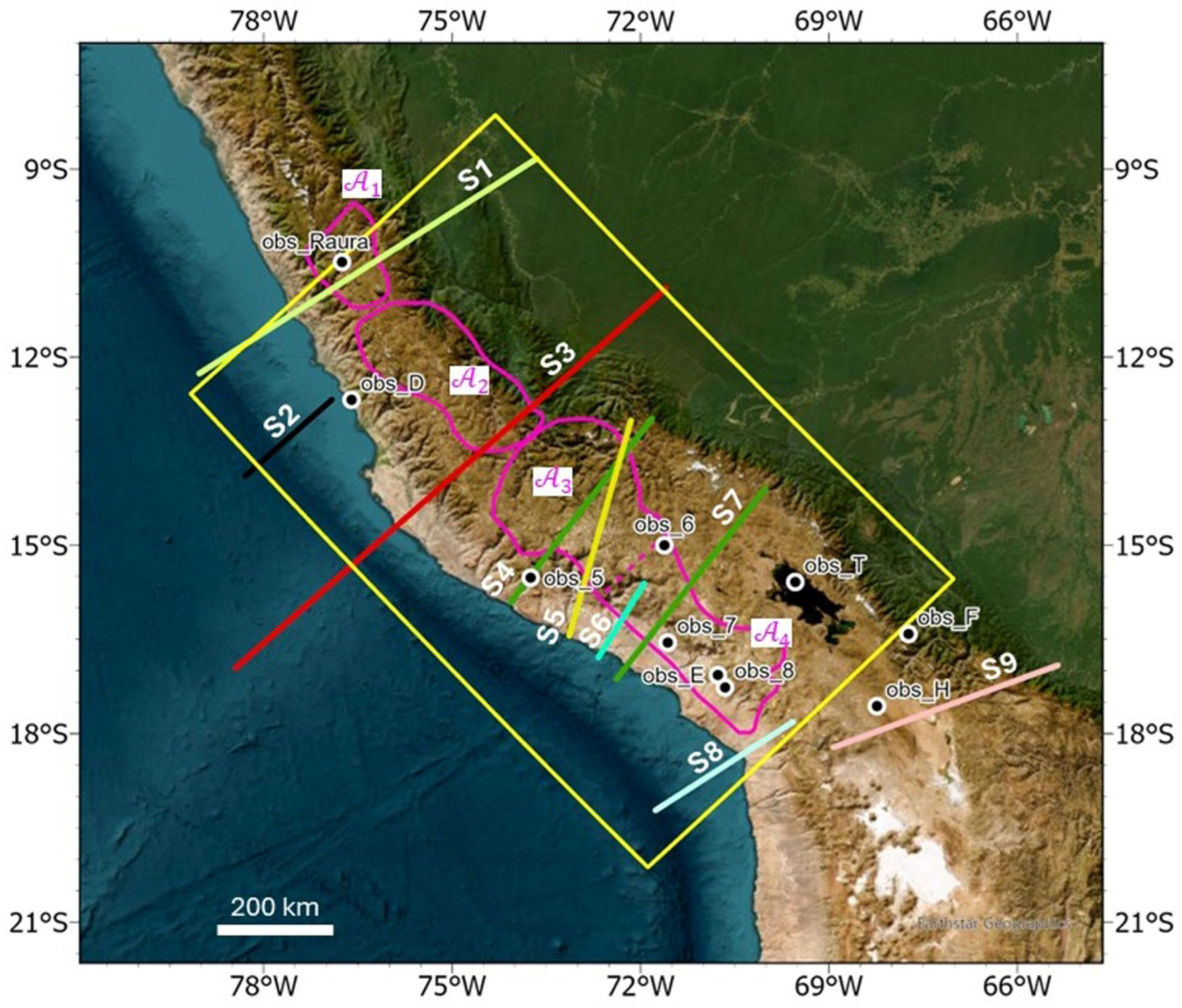
The study area (Figure 1) is located at the transition between the Northern Central Andes and the Central Andes Orocline, with the Nazca Ridge subduction zone marking the boundary between the two as well as the northern end of the active volcanic arc in Peru. The Peruvian forearc basin system between 8° S and 20° S (Figure 1) is an example of trench-parallel double forearc basins where seaward (slope) and landward (shelf) basins are separated from each other by the Outer Shelf High, a NW-trending structural culmination of the Precambrian–Paleozoic basement uplifted during the Neogene (Thornburg & Kulm, 1981 [20]; Kulm et al., 1982 [21]). The subduction beneath the Peruvian forearc of normal oceanic lithosphere and the buoyant Nazca Ridge, as well as the latter’s southward migration during the past 16–11 Myr (Hagen & Moberly, 1994 [22]; Hampel., 2002 [23]), have been associated with a wide range of effects on the leading edge of the overriding plate. In particular, rapid convergence is interpreted as driving subduction erosion and subsidence of the forearc area (von Huene & Lallemand, 1990 [24]; Clift et al., 2003 [25]), while slower rates of convergence were associated with its uplift and erosion. Major plate reorganization events were marked by significant changes in rate and direction of plate convergence (Herbozo et al., 2020 [26]) and paralleled periods of Andean orogeny like the mid-Eocene Incaic II (43–42 Ma) and middle to late Oligocene Aymara (30–27 Ma) contractional phases (Sébrier et al., 1988 [27]). The coastal sector of the Peruvian margin also includes the San Nicola batholiths, composed of Devonian plutonic bodies with compositions ranging from gabbro to monzogranite, which intrude the Precambrian basement and the Arequipa Massif (Mukasa and Henry, 1990 [28]).
According to Sempere et al. (2002) [29], the tectonic evolution of the Eastern Cordillera involved the inversion of an inherited rift system. This region was characterized by crustal shortening during the Oligocene–Miocene, affecting Paleozoic and Triassic–Jurassic extensional basins. The Peruvian Eastern Cordillera exposes the oldest Paleozoic lithologies within the Andean chain (Chew et al., 2016 [30]). Its southern sector is involved in the evolution of the Abancay Deflection, a major structural bend marked by a local change in strike to a NE–SW orientation (Gérard et al., 2021 [31]). This tectonic rotation occurred between the late Eocene and early Miocene and was associated with spatially variable exhumation (Roperch et al., 2006 [32]; Roperch et al., 2011 [33]; Gérard et al., 2021 [31]). The presence of this deflection strongly influenced regional paleogeography, producing marked differences between central and southern Peru. In particular, a late Eocene magmatic arc developed in the southern sector, whereas the northern sector experienced intense deformation without coeval magmatism (Carlotto et al., 2009 [34]; Roperch et al., 2011 [32]). The Western Cordillera can be subdivided into two main domains (Scherrenberg et al., 2014 [35]). The eastern domain corresponds to the Marañón fold-and-thrust belt, whereas the western domain is dominated by the Coastal Batholiths. The Marañón belt initiated during the Late Cretaceous and is characterized by tight folds toward the foreland and thrust faults toward the hinterland, with the entire system crosscut by NE–SW-striking, basement-involved strike–slip faults. During the Neogene, extensional tectonics, possibly related to crustal-scale yielding or episodic subduction decoupling, led to the development of intermontane basins such as the Ayacucho Basin (Wise et al., 2008 [36]). This basin is filled with volcanic and volcaniclastic deposits and records sedimentation punctuated by phases of shortening and erosion. The Coastal Batholiths consist of tabular intrusive bodies with an estimated thickness of approximately 5 km (Haederle and Atherton, 2002 [37]). They represent a major expression of Mesozoic magmatism in Peru and are associated with the Mochica phase of deformation (Pfiffner and Gonzalez, 2013 [38]). Several super-units have been identified within the batholith, each characterized by distinct compositions ranging from gabbro–diorite to granite and separated by well-defined contacts.
Figure 1. Relief and bathymetric map (from ERSI: https://www.esri.com/en-us/home) of the study area (boxed) and surrounding region, showing location of the considered profiles and of deep boreholes providing heat flow data relevant for this study (referred to site identification in Table 1). The four geothermal regions identified by magenta contours, constraining a SE-ward increase in mantle heat-flow (Qm) values, are as follows: A1—Churin, A2—Central, A3—NE Ejes Volcánico Sur, and A4—SO Ejes Volcánico Sur (Vargas and Cruz, 2010 [39]).
Geosciences 16 00216 g001
Table 1. Surface Heat Flow Sites in Peru from Uyeda et al. (1980) [40], Uyeda and Watanabe (1982) [41], Henry and Pollack (1988) [42] and Sclater et al. (1970) [43].
AcronymSite NameS LatW LongObserved Qs
(mW·m−2)
obs_RauraRaura10°29′76°45′30 ± 6.0[40,41]
obs_DCondestable12°41′76°36′38 ± 3.8[41]
obs_5Marcahui15°31′73°45′50 ± 10.0[42]
obs_6Tintaya14°54′71°21′40 ± 6.0[42]
obs_7Cerro Verde16°33′71°34′52 ± 5.2[42]
obs_8Toquepala17°16′70°39′75 ± 3.8[42]
obs_ECuajone17°04′70°46′66 ± 9.9[42]
obs_FChojilla16°25′67°44′76 ± 7.6[42]
obs_HChacarilla17°34′68°14′73 ± 14.6[42]
obs_TTiticaca Lake (Isla Soto)15°35′69°32′75 ± 15.0[43]

3. Methods and Outputs

3.1. 3D Main Geological Surfaces and Moho Discontinuity

The reconstruction of 3D surfaces was performed through the spatial interpolation of stratigraphic constraints derived from nine interpreted geological cross-sections. Within the continental domain, modeling focused on the primary stratigraphic interfaces, namely the sediment–basement boundary and the crust–mantle transition. The depths to the top-basement and the Moho were interpolated in order to quantitatively constrain the thickness distribution of both the sedimentary cover and the crystalline basement (which is between the Moho to the top-basement surface). Conversely, for the subducting slab, only the upper interface was considered, as it represents the primary geometrical constraint for defining slab geometry.
The cross-sections were georeferenced by GIS (Esri Inc., 2025 [44]), including a consistency check between the structural architecture and lithostratigraphic relationships depicted in the sections and the corresponding geological–structural outcrop patterns. This validation ensured coherence between subsurface interpretations and surface geology. Consequently, the depth data extracted from the cross-sections were automatically projected into a common spatial reference system and integrated into a unified geodatabase.
To accurately resolve the geometry of the modeled interfaces, point sampling along the cross-sections was performed using a non-uniform spacing. This adaptive sampling strategy was designed to increase point density in sectors characterized by high geometric complexity and high thickness gradient, while maintaining a lower density in more homogeneous regions. Such an approach minimizes interpolation artifacts and improves the fidelity of the reconstructed surfaces, particularly in structurally complex domains.
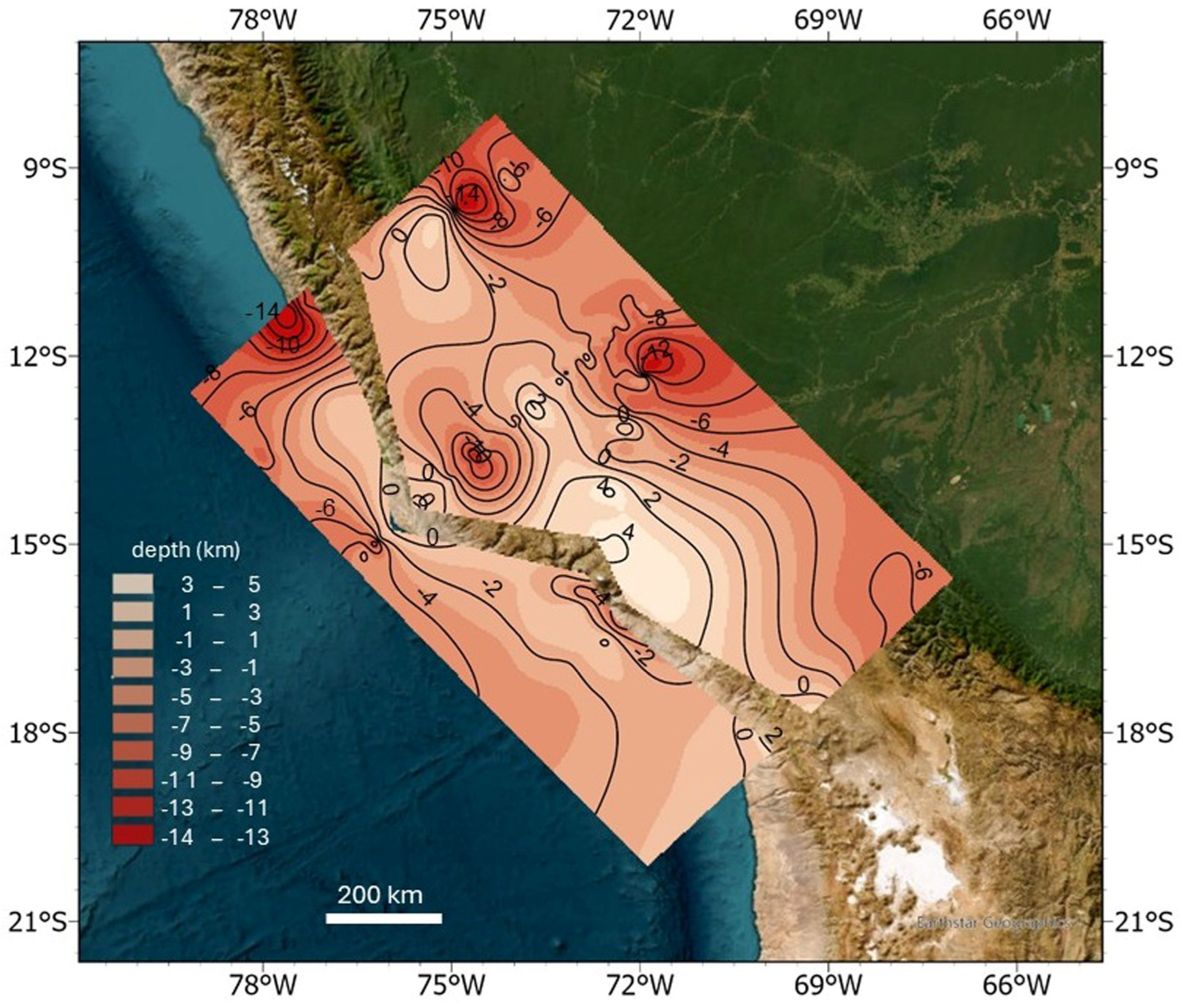
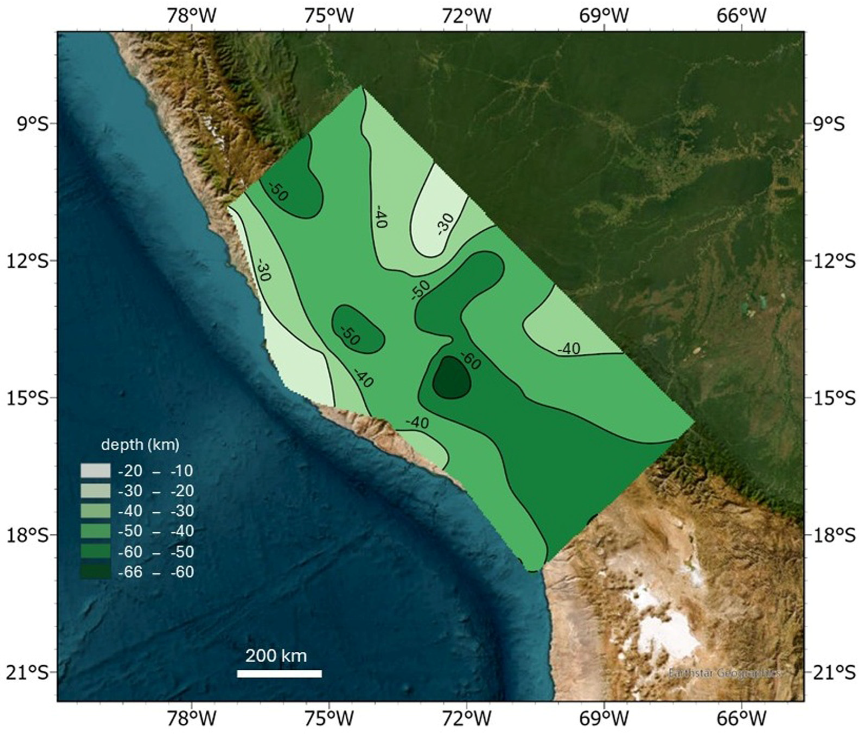
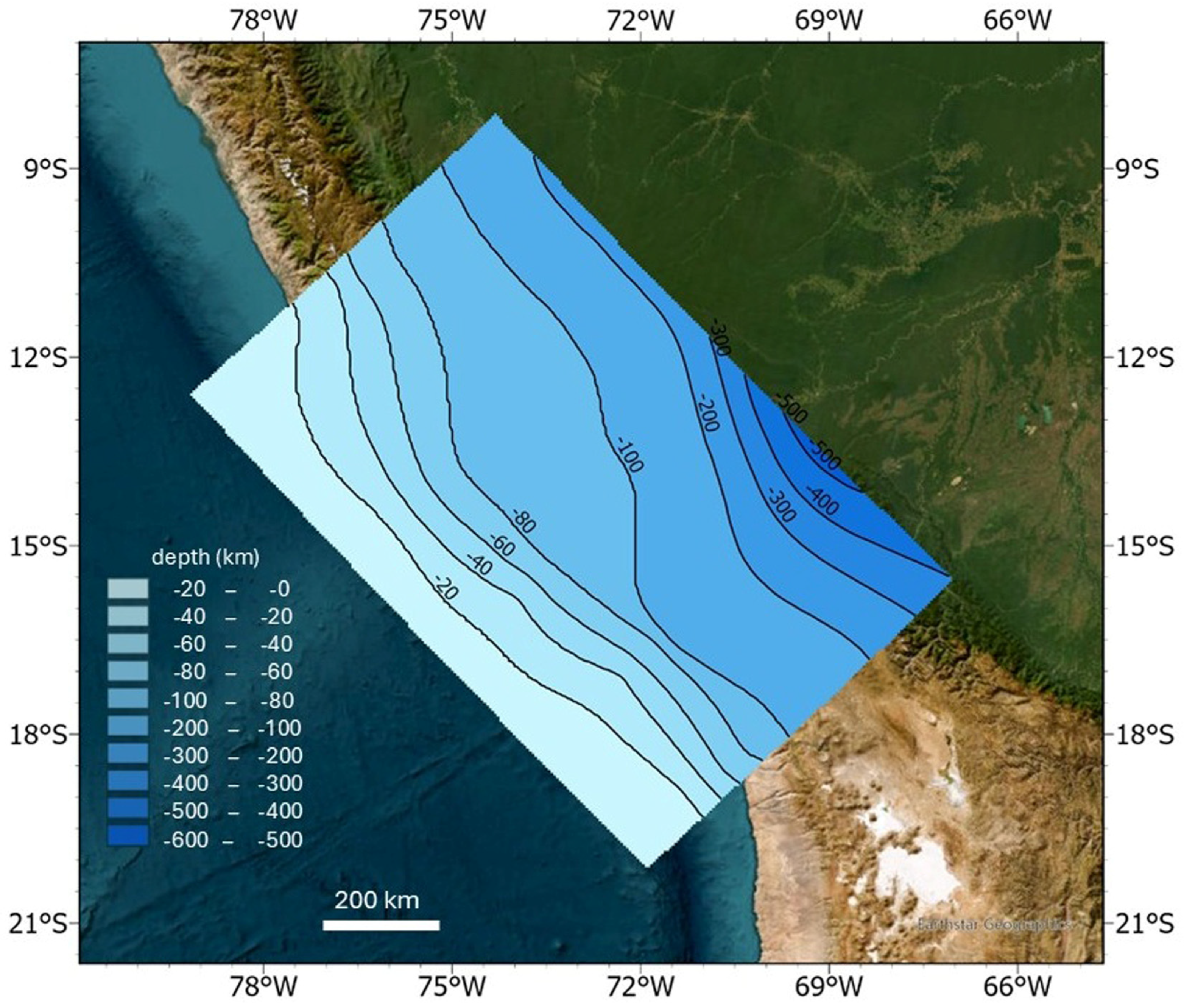
The interpolated datasets were subsequently used to generate continuous raster surfaces representing the main geological interfaces. Specifically, raster grids were produced for the bottom of the sedimentary cover (Figure 2), the bottom of the basement (Figure 3), and the top of the subducting slab (Figure 4). These surfaces provide a consistent three-dimensional structural framework of the study area and constitute the basis for quantitative analyses.
For the sedimentary cover, the interpolation was performed over two distinct spatial domains (Figure 2). This subdivision was required due to the presence of a basement outcrop, extending approximately NW–SE and subparallel to the coastline in the onshore sector (Figure 1). The occurrence of exposed basement interrupts the lateral continuity of the sedimentary succession, thus necessitating separate interpolation domains to avoid spurious extrapolation across non-depositional areas. The basement surface (Figure 3) was spatially constrained to regions where the Mohorovicic discontinuity (Moho) is defined, thereby ensuring consistency with the crustal-scale structural framework. The slab top surface (Figure 4) was reconstructed by interpolating depth constraints derived from the nine cross-sections in locations where the slab interface was explicitly identified. These constraints were integrated with regional-scale information provided by the 100–500 km depth contour lines from Hayes et al. (2018) [45], thereby incorporating independent geophysical constraints into the interpolation procedure. The resulting surface provides a geometrically consistent representation of the slab architecture across the study area, compatible with previously published slab models.
Figure 2. Interpolated top-basement isobaths obtained from 3D modelling based on the geological sections of Figure 5.
Geosciences 16 00216 g002
Figure 3. Interpolated upper plate Moho isobaths obtained from 3D modelling based on the geological sections of Figure 5.
Geosciences 16 00216 g003
Figure 4. Interpolated top-slab isobaths obtained from 3D modelling based on the geological sections of Figure 5.
Geosciences 16 00216 g004
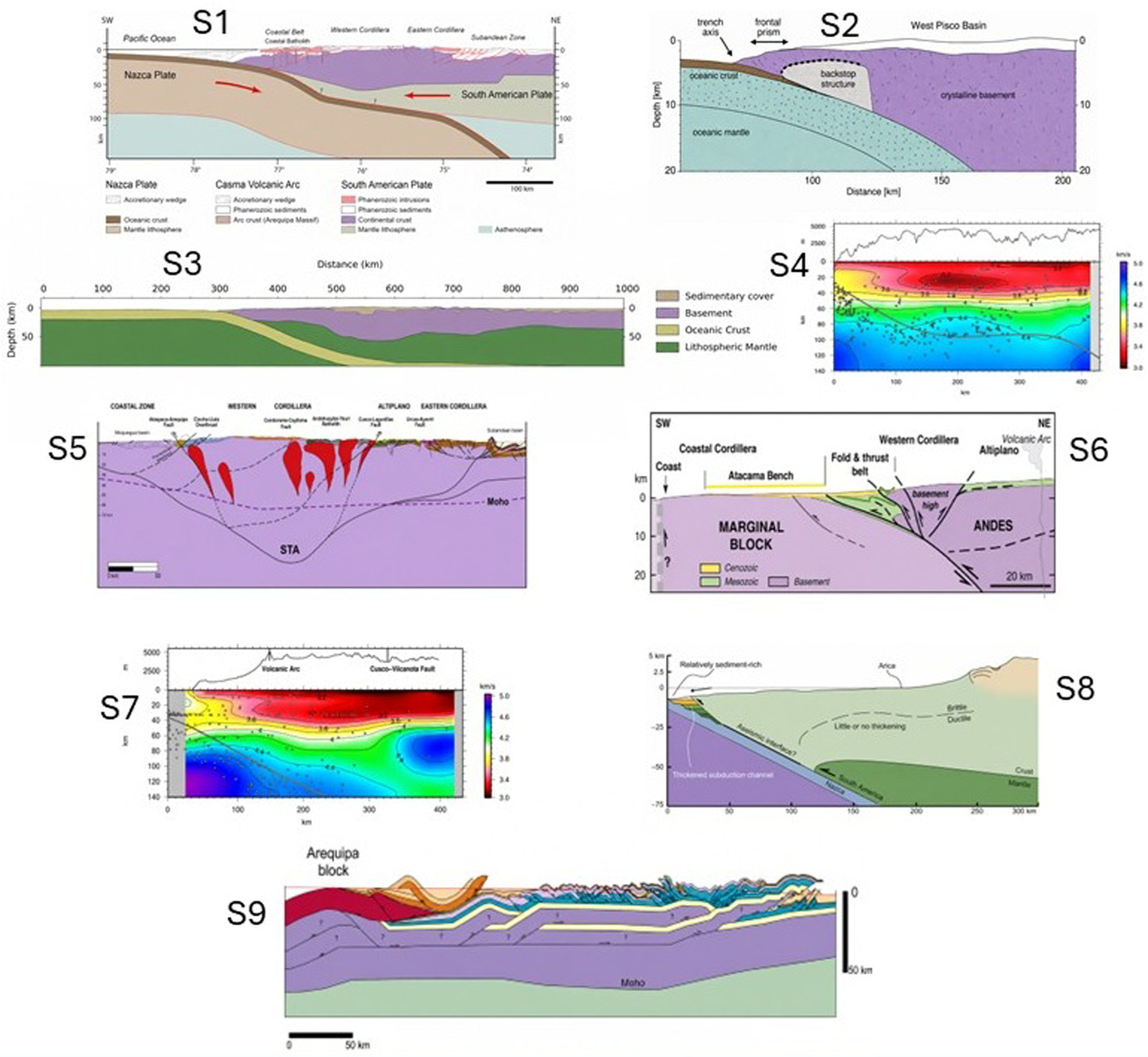
Figure 5. Published geological and seismic tomography profiles selected for this study, as modified from the following authors. S1: Adrian Pfiffner and Oscar Gonzalez (2013) [38]; S2: Krabbenhoft et al. (2004) [46]; S3: Ciattoni et al. (2025) [47]; S4: Ma and Clayton (2014) [48]; S5: Carlotto et al. (2023) [49]; S6: Armijo et al. (2015) [50]; S7: Ma and Clayton (2014) [48]; S8: Madella et al. (2016) [51]; S9: Hildebrand and Whalen (2014) [52].
Geosciences 16 00216 g005

3.2. Thermal Modelling

To define the heat flow map, we constructed a regular grid of 96 pseudo-wells spatially distributed across the entire study area. The pseudo-wells were placed at 90.5 km spacing along the NE–SW direction and 114.1 km apart in the orthogonal direction, ensuring a uniform coverage of the region under investigation. This grid configuration allowed for a representation of spatial variations in heat flow across the study area, by calculating Q s at each pseudo-well and interpolating the resulting data.
In the computation of the surface heat flow Q s , we considered (i) the contribution of the mantle heat flow Q m , (ii) the radiogenic heat Q S C in the sedimentary cover and Q B in the basement, and (iii) the frictional heat Q F in the megathrust zone, obtaining the following equation:
Q S =   Q + Q S C + Q B
In the equation, Q represents the heat flow at the base of the model due to the heat flow coming from the mantle and to the frictional heat of the thrust when it is present.
For the megathrust zone, we considered Q = ( Q o + Q F ) S 1 , where Q o is the oceanic mantle heat flow and S = 1 + b z f   v   s i n δ κ , with b 1 , is the reducing divisor near the megathrust fault [53]. For the continental zone, we considered Q =   Q m . Instead, Q S C =   H S C h S C is the contribution of the sedimentary layer considering a constant radiogenic source [54,55,56], while Q B =   H B D 1   e h B D is the contribution of the basement considering a radiogenic source with an exponential trend [57,58,59]. Considering a constant radiogenic source, we obtain the following temperature in the sedimentary cover layer:
T S C z = T S + Q S k S C z z t H S C 2 k S C z z t 2
where T S is the surface temperature.
Considering a radiogenic source with an exponential trend, we obtain the following temperature in the basement:
T B z = T B + Q   k B z z t h S C + H B D 2 k B 1   e z z t h S C D
where T B is the temperature at basement top and D is the depth scale.
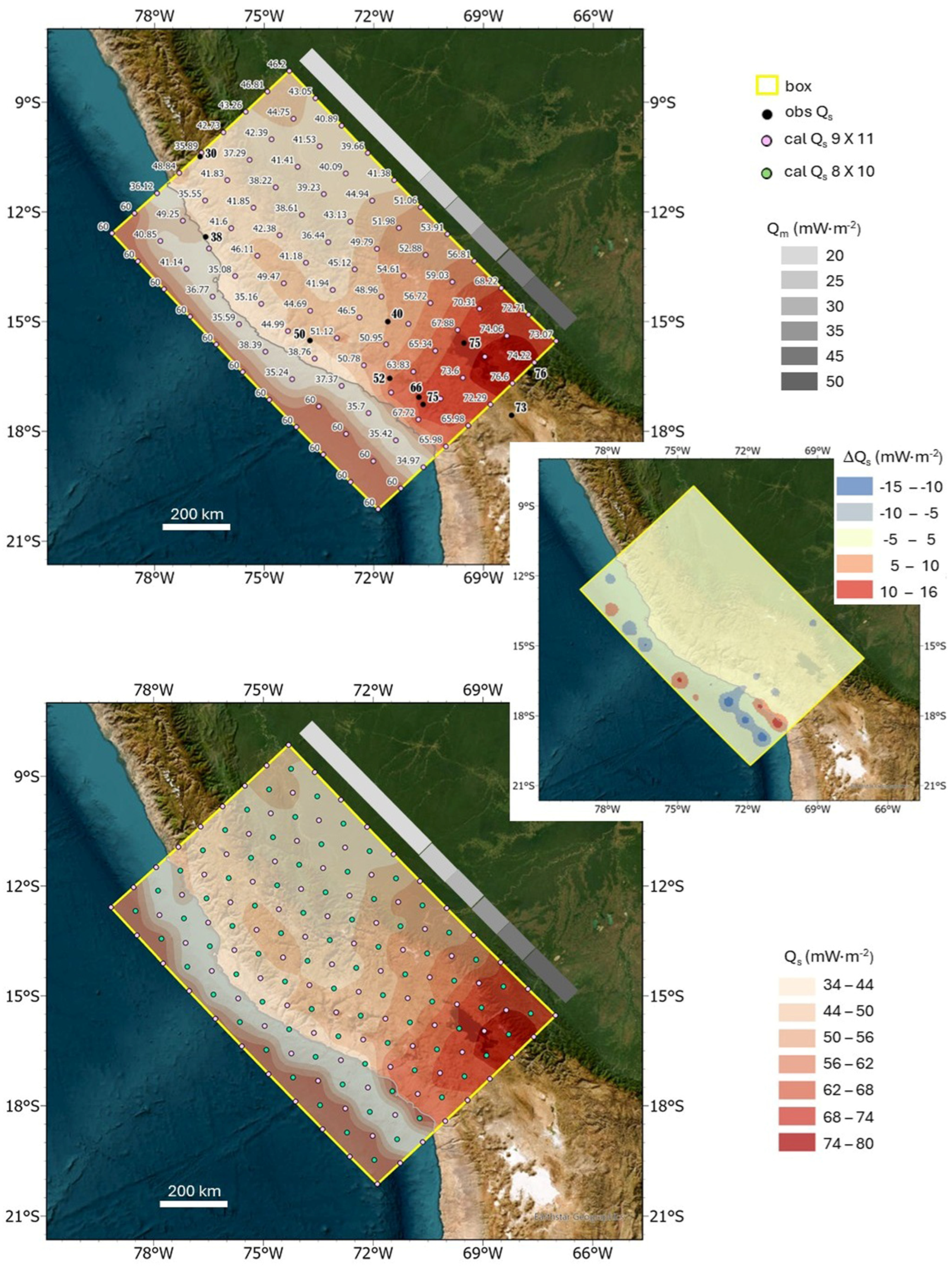
As a first-order approximation, surface heat flow was calculated at 99 equally spaced pseudo-wells distributed across the study area (upper panel of Figure 6). The adoption of a regular grid was primarily motivated by the heterogeneous and spatially limited distribution of the available geological and thermal constraints. Despite these limitations, the existing dataset is considered sufficient to constrain the first-order thermal structure and the regional distribution of heat flow within the investigated area. The thickness of the layers was derived from interpolation maps, whereas the thermal parameters adopted in the calculations are summarized in Table 2.
An additional aspect to consider in the analytical calculation of surface heat flow is the value assigned to Qm, which is not uniform across the study area and, in some locations, increases markedly toward the southeast (Hamza and Munoz, 1996 [67]; Vargas and Cruz, 2010 [39]; Hamza and Viera, 2012 [66]). To account for this spatial variation, we assumed a progressive increase in Qm from the northwest to the southeast, as illustrated in Figure 6.
The interpolation of the heat-flow datasets was performed using kriging method, a geostatistical technique particularly suitable for spatially correlated variables. This method is able to account for the spatial continuity of the data through variogram analysis. Compared to simpler deterministic interpolation methods, kriging allows both regional trends and local variations to be reproduced more realistically.
To assess whether the resulting surface heat-flow pattern was independent of the adopted grid configuration, a new set of calculations was performed by using a second grid composed of 80 pseudo-wells. In this configuration, each pseudo-well was positioned at the center of the cells defined by the previous grid (lower panel of Figure 6), thus allowing the spatial sampling to be shifted relative to the first setup. Comparison between the results obtained from the two independent grids—of 99 and of 80 pseudo-wells—indicates that the overall heat-flow pattern remains substantially unchanged, supporting the conclusion that the modelled distribution is not significantly influenced by the choice of grid geometry or by the positioning of the pseudo-wells. Nevertheless, some local differences emerge in the offshore sector, where the calculated heat-flow values display stronger lateral variations.
An additional calculation was performed by combining the two pseudo-well grids into a single dataset of 179 pseudo-wells (lower panel of Figure 6). The resulting heat-flow distribution confirms the persistence of the main regional trend identified in the previous results, while highlighting the higher heat-flow variations in the offshore area, although with a more limited spatial extent (right panel of Figure 6).
All interpolation results consistently indicate an increase in surface heat flow toward the southeastern portion of the study area, as well as an abrupt lateral variation across the offshore sector.
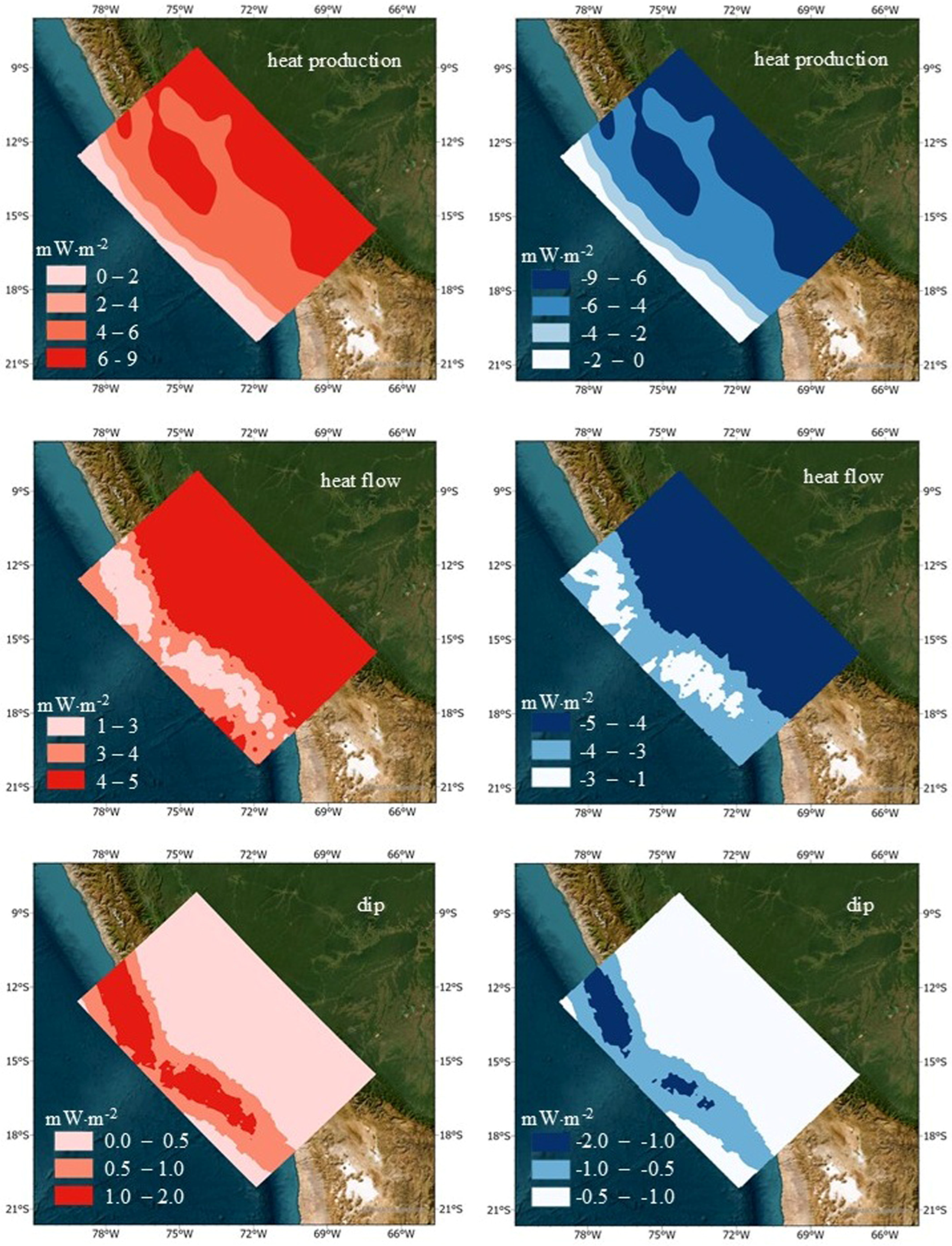
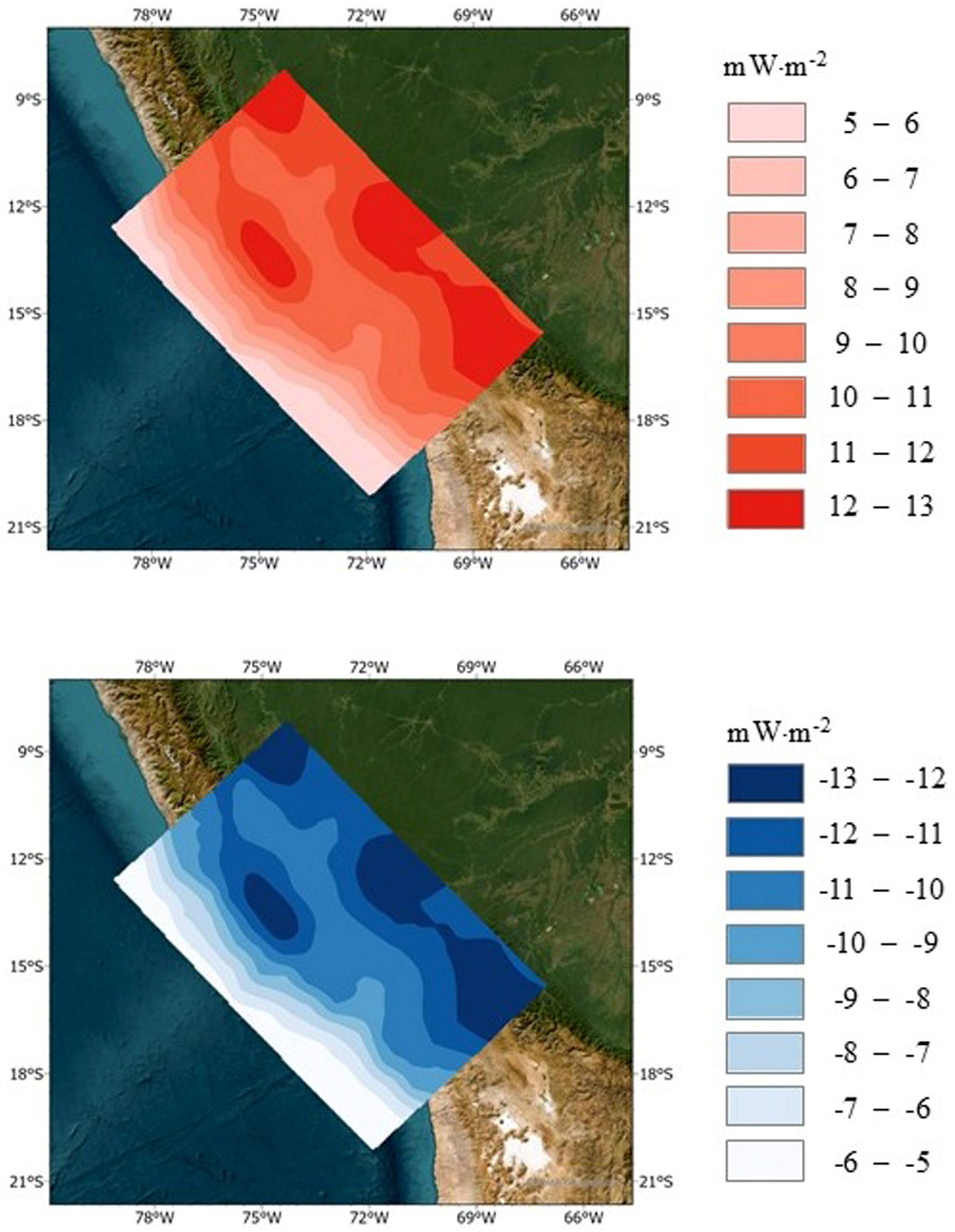
To assess the sensitivity of the calculated surface heat-flow distribution, a series of tests was performed by varying radiogenic heat production, slab dip, and basal heat-flow around the reference model values. This approach was used to evaluate how changes in the adopted thermal and geometrical parameters affect both the absolute heat-flow values and the overall spatial pattern of the results. Variations in radiogenic heat production and basal heat flux input directly influence the modelled surface heat flux distribution. Specifically, an increase or decrease in radiogenic heat production values, as well as an in basal heat flux, results in a corresponding increase or decrease in surface heat flux values, with the largest differences observed in the innermost sector of the study area. In contrast, variations in plate inclination produce an opposite thermal response. An increase in slab dip leads to a decrease in the modelled surface heat flow, whereas a lower inclination results in higher surface heat-flow values (Figure 7). Finally, Figure 8 summarizes the maximum and minimum variations in surface heat flow obtained from the complete set of sensitivity tests, considering the full range of values adopted for the three investigated parameters.

4. Main Outcomes of the Study

The top of the basement in the study area (Figure 2) is characterized by highs and lows which are controlled by the inherited Paleozoic and younger extensional basin architecture, as well as by pre-Andean mountain building processes and later overprinting by basement-involved Andean shortening, tectonic inversion and thick-skinned thrusting (e.g., Ciattoni et al., 2025 [47] and references therein). The pattern emerging from Figure 2 is consistent with the well known observation that the basement structure in the Central Andes is strongly affected by major fault systems and crustal discontinuities that segment the region into distinct tectonic domains (e.g., Ramos et al., 2002 [68]; Ramos and Folguera, 2009 [69]). In particular, basement uplifts that characterize the Coastal Cordillera and, in the northern-central sector of the study area, also the thick-skinned Eastern Cordillera (Ciattoni et al., 2025 [47]) are well defined by outcropping/elevated basement sectors in Figure 2.
Moho depths vary significantly within the study area, both across and along strike (Figure 3). Beneath the forearc region, the crust is relatively thin, and the Moho typically lies at depths of approximately 30–40 km, consistent with a tectonically eroded and mechanically thinned margin. Moving eastward beneath the Western Cordillera and the volcanic arc, the Moho deepens substantially, reflecting crustal thickening driven by magmatic underplating and long-term shortening. The greatest crustal thickness is observed beneath the Altiplano, where Moho depths commonly exceed 60–70 km, forming a broad crustal root that supports the elevated topography of the plateau. Importantly, the Moho geometry is not smoothly varying but instead shows pronounced lateral heterogeneity in three dimensions. Deep geological sections and geophysical imaging (Figure 5) reveal step-like offsets, uplifts and depressions of the Moho that correlate with major tectonic domains and upper crustal fault systems.
In the study area, the geometry of the subducting Pacific slab—represented by the downgoing Nazca Plate—exhibits a distinctly three-dimensional configuration, characterized by significant variations in dip angle and along-strike geometry down to depths of ~100 km (Figure 4). A key feature of the slab geometry in the study area is its along-strike variability, particularly at the transition between two major segments of the Andean margin. Northward, toward central Peru, the slab flattens into a low-angle (flat-slab) configuration, whereas to the south, toward northern Chile, it maintains a steeper angle of dip. The three-dimensional shape of the slab is further complicated by the occurrence of the major bathymetric feature on the oceanic plate represented by the aseismic Nazca Ridge. Southeast of the latter, the slab begins its descent at relatively low angles, typically on the order of ~25–30°, offshore and beneath the forearc region. As it progresses inland beneath the Western Cordillera, the slab steepens to dips of ~30–45°, facilitating the emplacement of a thick mantle wedge above it. At greater depths (beyond ~100–150 km), the slab continues to descend into the mantle relatively smoothly eastward (Figure 4).
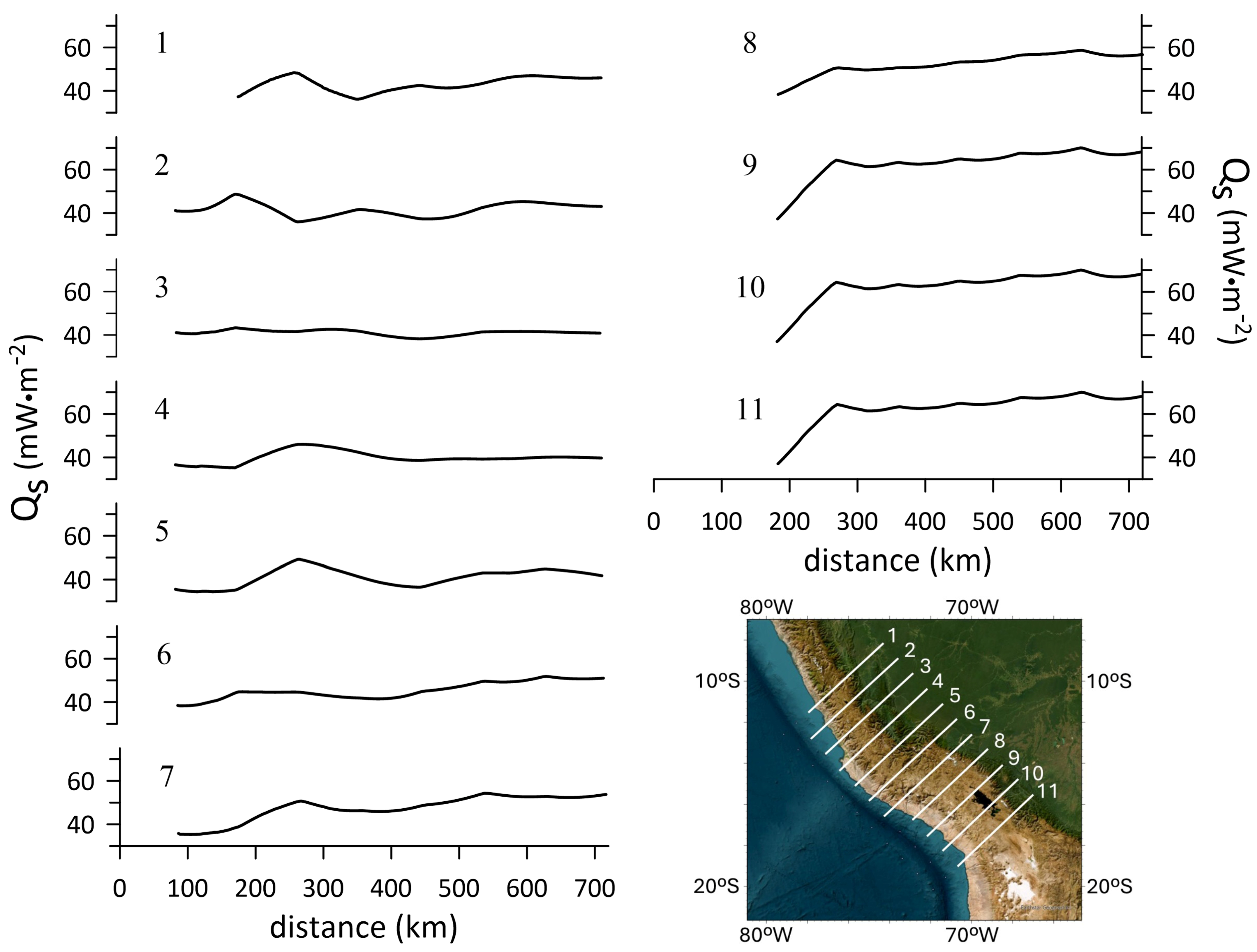
The thermal structure of the study area, obtained by the analytical method used in this study, is shown in the lower panel of Figure 6. The southern portion of the study area is characterized by a NW-SE trending Qs minimum located immediately NE of the subduction trench, beneath the accretionary wedge (where the oceanic slab is buried by accreted sediments). This minimum expands to the north, encompassing most of the Andean belt (including both Western and Eastern Cordilleras) as well as the foreland of the Andean retrowedge to the NE (i.e., the South American continent). The overriding plate displays a gradual increase in Qs moving from NW to SE (Figure 6).
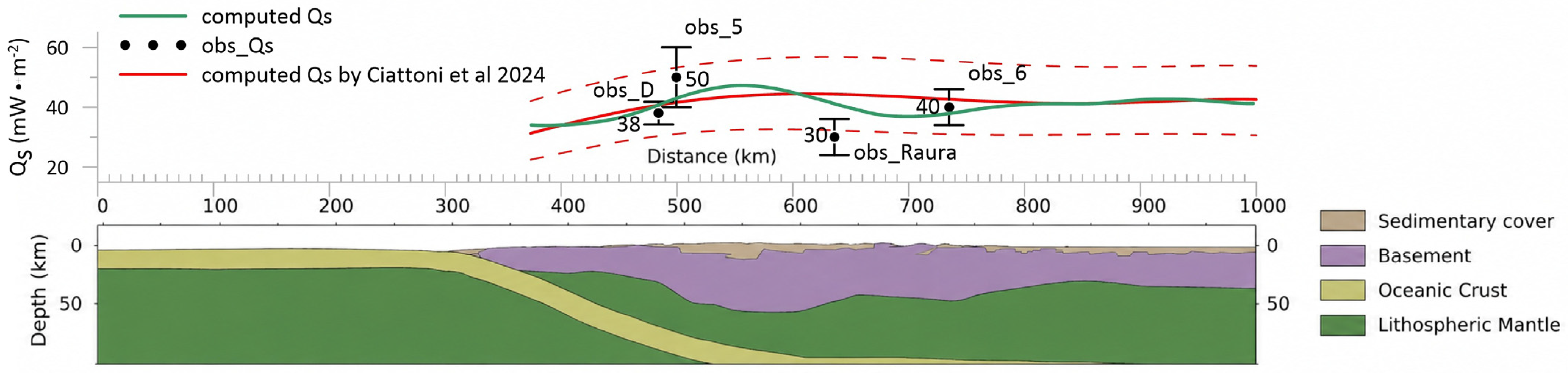
Both trends are clearly visible in the Qs profiles of Figure 9. The new 3D results of this study are generally consistent with those (2D) obtained in a previous study of a deep geological section across the study area; however, they define thermal maxima and minima with enhanced detail along the same section (Figure 10). The new results define a relative Qs minimum over the Eastern Cordillera and the eastern Andean thrust front, while relative maxima occur over the Western Cordillera and the South American foreland to the NE. Comparison with available temperature data obtained from deep boreholes show a good fit between calculated and measured data (Figure 10).

5. Discussion

The 3D structural and thermal model presented here provides new constraints on the crustal architecture and geodynamic evolution of the Central Andes that were not re-solvable in previous 2D studies. In particular, the integration of basement morphology, Moho geometry, slab configuration, and thermal structure reveals significant lateral variability and segmentation, offering a more realistic representation of lithospheric processes.
The reconstructed basement topography (Figure 2) is characterized by structural highs and lows that likely extend into the lower crust, consistent with previous interpretations (Ciattoni et al., 2025 [47]). In contrast to earlier 2D approaches, the 3D model highlights the spatial continuity and segmentation of these features, suggesting that inherited basement heterogeneities play a key role in controlling both deformation and heat distribution. These structures, rooted in the Proterozoic metamorphic framework of the Amazonian craton margin (Mukasa and Henry, 1990 [28]; Romero et al., 2013 [72]), act as long-lived zones of crustal weakness that localize strain and potentially influence fluid circulation. In addition, these inherited discontinuities likely act as preferential permeability pathways that facilitate vertical magma ascent, thereby linking deep mantle melting regions to shallow crustal heat anomalies and contributing to localized increases in surface heat flow (Qs).
The geometry of the Moho (Figure 3) further demonstrates the added value of the 3D approach. Rather than a laterally uniform interface, the Moho exhibits pronounced depth variations and along-strike segmentation, reflecting the combined effects of crustal shortening, magmatic underplating, and lithospheric modification. These processes have been widely invoked in the Central Andes (e.g., Hayes et al., 2018 [45]), but the 3D model allows their spatial distribution to be resolved more clearly. Variations in Moho depth can be linked to differential magmatic addition and possible lower crustal flow or redistribution, providing new constraints on crustal growth mechanisms and lithospheric strength. Importantly, regions of Moho shallowing spatially correlate with higher modeled Qs values, suggesting enhanced advective heat transfer from mantle-derived magmas and underplated material, which can elevate lower crustal temperatures to >700–800 °C and contribute significantly to the regional thermal budget.
The relationship between slab geometry and the thermal structure of the overriding plate is also refined. Previous studies have established the first-order control of slab dip on magmatism and deformation (e.g., Gutscher et al., 2000 [73]; Ramos et al., 2002 [68]; Horton, 2018 [74]; Horton et al., 2022 [75]), but the 3D model shows how these effects are expressed as laterally continuous thermal gradients rather than abrupt transitions. The modeled Qs distribution (Figure 9) reveals a systematic increase from flat-slab to steep-slab domains, consistent with variations in mantle wedge development and magmatic input. This pattern can be quantitatively linked to mantle wedge thermal structure, where temperatures in the wedge increase from <900 °C in flat-slab regions to >1100–1200 °C in steep-slab settings, exceeding the solidus of hydrated peridotite and enabling partial melting.
In addition to slab dip geometry, the transition from flat- to steep-slab subduction along the Central Andes can be quantitatively interpreted in terms of competing forces controlling slab buoyancy and bending. The subduction of the Nazca Ridge introduces a positive buoyancy anomaly associated with thickened oceanic crust (up to ~15–20 km compared to normal ~7 km) and reduced average slab density, which decreases slab pull forces and promotes slab flattening. This buoyancy effect can be approximated by a reduction in negative slab buoyancy on the order of 10–20%, sufficient to inhibit slab descent into the mantle and maintain a shallow dip angle. However, this effect is modulated by convergence rate, which in the Central Andes ranges from ~6 to 8 cm/yr (Ramos et al., 2002 [69]); higher convergence velocities increase viscous drag and enhance downward slab forcing, counteracting ridge buoyancy and favoring re-steepening of the slab. Furthermore, lithospheric strength contrasts between the overriding South American plate and the subducting Nazca plate exert an additional control on slab geometry. A stronger, thicker continental lithosphere increases interplate coupling and promotes horizontal slab underthrusting, whereas localized weakening—potentially associated with thermal erosion or inherited structural discontinuities—facilitates slab rollback and steepening. These effects can be expressed in terms of effective elastic thickness (Te), where values exceeding ~40–50 km favor flat-slab configurations, while reduced Te (<30–35 km) allows greater slab flexure and descent. The balance between ridge buoyancy, slab pull, viscous resistance, and overriding plate strength therefore defines a dynamic regime in which flat-slab segments are transient features that evolve toward steeper configurations once the buoyant ridge has fully subducted or thermal weakening reduces plate coupling. This dynamic framework is consistent with the observed spatial distribution of Qs, as flat-slab regions correspond to reduced mantle wedge thickness and suppressed asthenospheric flow, while steep-slab domains reflect the re-establishment of mantle wedge circulation and associated heat transport. Consequently, the lateral variability in thermal structure identified in the 3D model can be directly linked to these quantitatively constrained geodynamic parameters, providing a more physically robust explanation for along-strike segmentation of magmatism and heat flow.
In the northwestern sector, low Qs values correspond to flat-slab subduction, where the absence of a well-developed mantle wedge suppresses partial melting and limits magmatic activity (Gutscher et al., 2000 [73]). In these regions, slab dehydration reactions occur at relatively shallow depths (~70–100 km), but the thermal regime is insufficient to induce widespread flux melting in the overlying mantle due to low wedge temperatures. Moving southwestward, the transition to a more inclined slab geometry is associated with intermediate Qs values and moderate thermal conditions, reflecting limited mantle upwelling. Here, dehydration reactions shift to greater depths (~100–150 km), increasing fluid flux into a progressively hotter mantle wedge (≈950–1050 °C), which promotes localized partial melting and moderate magma production.
In southern Peru, particularly in the Arequipa region and along the Colca volcanic zone, high Qs values coincide with a steeply dipping slab and a well-developed volcanic arc (Voos et al., 2026 [76]). Here, enhanced mantle melting generates significant magmatic activity, driving high-temperature hydrothermal systems. This can be quantitatively interpreted as the result of slab-derived fluid release at depths of ~120–180 km, where the overlying mantle wedge reaches temperatures above 1100 °C, conditions sufficient for significant degrees (>10–15%) of partial melting. The resulting buoyant magmas ascend through structurally controlled pathways, with ascent rates and magma flux influencing the magnitude of advective heat transport into the crust. The highest Qs values occur toward the Peru–Bolivia border, where persistent steep subduction supports sustained magma generation and pronounced thermal anomalies, consistent with observations from geothermal systems such as Tutupaca (Steinmüller, 2001 [77]). In these regions, repeated magma intrusion and possible magma ponding at mid-crustal levels (~15–25 km depth) further enhance conductive and advective heat transfer, maintaining elevated surface heat flow.
Compared to previous 2D thermal models, the 3D framework demonstrates that thermal anomalies are spatially focused and structurally controlled. Areas of elevated temperature are not uniformly distributed along the arc but are concentrated where favorable slab geometry, crustal structure, and magmatic processes coincide. This has important implications for geothermal systems, as it suggests that the most significant geothermal resources are localized within specific structural and thermal domains rather than broadly distributed along strike. Moreover, the coupling between mantle melting conditions, fluid release depth, and magma ascent efficiency provides a quantitative basis for predicting where significant heat flow anomalies are most likely to occur.
The integration of thermal and structural information also provides new insights into structural permeability distribution. Zones where high Qs values overlap with basement discontinuities and Moho irregularities are likely to enhance fluid circulation and reservoir fluid storage potential. This represents a significant advance over previous models, which could not simultaneously resolve heat sources and structural controls in three dimensions. From an applied perspective, the 3D thermal model provides a crustal-scale reference framework for resource exploration. By identifying areas where favorable thermal conditions coincide with structurally controlled permeability, the model can help guide geothermal exploration and reduce uncertainty in targeting. More broadly, such a framework may also support studies of mineral systems and basin evolution, complementing existing approaches (e.g., Invernizzi et al., 2014 [78]; Maffucci et al., 2015 [79]; Filipovich et al., 2020 [80]).
Beyond geothermal implications, our results contribute to a better understanding of lithospheric processes in the Central Andes. The spatial correlation between Moho relief, slab geometry, and thermal gradients supports a heterogeneous model of crustal evolution, in which magmatic addition, crustal thickening, and possible lower crustal flow are modulated by both inherited structures and ongoing subduction dynamics (Hayes et al., 2018 [45]; Scire et al., 2016; 2017 [81,82]). The addition of quantitative constraints on mantle wedge temperature, dehydration depth, and melt generation further reinforces this interpretation, demonstrating that along-strike segmentation of the orogen reflects not only geometric variations in slab configuration but also systematic differences in thermo-petrological conditions governing magma production and heat transfer. This helps explain the pronounced segmentation of the orogen and the variability in tectonic and magmatic processes along strike.
In summary, the transition from 2D to 3D modeling enables a more integrated and spatially consistent interpretation of the relationships among tectonics, magmatism, and thermal structure. By explicitly coupling surface heat flow with mantle wedge thermal state, slab dehydration processes, magma ascent pathways, and the dynamic balance between ridge buoyancy, convergence rate, and lithospheric strength, the model provides a more physically grounded representation of the Central Andes lithosphere and offers new quantitative constraints on both geodynamic processes and geothermal resource potential.

6. Conclusions

(1)
The three-dimensional geometry of the Moho beneath southern Peru is a fundamental feature of the regional geodynamic system, reflecting the interplay of subduction dynamics, crustal thickening, magmatism, and inherited crustal heterogeneity. Its complex and laterally variable form provides key insights into the processes shaping the Central Andes and highlights the importance of 3D approaches for accurately characterizing lithospheric structure at active continental margins.
(2)
The northwest–southeast increase in Qs values across central-southern Peru reflects a fundamental control exerted by slab geometry on mantle processes. Flat-slab subduction in the northwestern sector of the study area suppresses heat transfer and magmatism, whereas progressively steeper subduction moving to the southeast promotes mantle melting, volcanic activity, and enhanced geothermal activity at the surface. This along-strike variation provides a coherent framework for understanding the distribution of geothermal resources and the thermal structure of the Andean margin.

Supplementary Materials

The following supporting information can be downloaded at: https://www.mdpi.com/article/10.3390/geosciences16060216/s1.

Author Contributions

Conceptualization, S.M., A.M. and S.S.; methodology, S.M., A.M. and S.S.; software, A.M.; validation, A.M., S.M. and S.S.; formal analysis, A.M. and S.S.; investigation, S.M., A.M. and S.S.; resources, A.M. and S.S.; data curation, A.M., S.M. and S.S.; writing—Original draft preparation, A.M.; writing—Review and editing, S.M.; visualization, A.M.; supervision, S.M. and S.S.; project administration, S.S.; funding acquisition, S.S. All authors have read and agreed to the published version of the manuscript.

Funding

Financial support for this research was provided by the Italian Ministry of University and Research (MUR) through the PRIN 2022 call (ranking list advancement; D.D. 1401/2024)—Project title: “ITAL—Innovations in Thermochronology applied to the Andean natural laboratory” (code 20225Z84SN, CUP J53C24002940006) to Stefano Mazzoli.

Data Availability Statement

Computed data can be found in attached Supplementary Materials File.

Acknowledgments

The authors are grateful to the editor for his helpful support in organizing the manuscript. Thoughtful and constructive reviews by two anonymous referees allowed us to substantially improve the manuscript.

Conflicts of Interest

The authors declare no conflicts of interest.

References

  1. Ranalli, G. Rheology of the Earth; Chapman & Hall: London, UK, 1995. [Google Scholar]
  2. McKenzie, D.; Jackson, J.; Priestley, K. Thermal structure of oceanic and continental lithosphere. Earth Planet. Sci. Lett. 2005, 233, 337–349. [Google Scholar] [CrossRef]
  3. Grose, C.J.; Afonso, J.C. Comprehensive plate models for the thermal evolution of oceanic lithosphere. Geochem. Geophys. Geosyst. 2013, 14, 3751–3778. [Google Scholar] [CrossRef]
  4. Morgan, P.; Sass, J.H. Thermal regime of the continental lithosphere. J. Geodyn. 1984, 1, 143–166. [Google Scholar] [CrossRef]
  5. Royden, L.H. The steady-state thermal structure of eroding orogenic belts and accretionary prisms. J. Geophys. Res. 1993, 98, 4487–4507. [Google Scholar] [CrossRef]
  6. Brown, M. P–T–t evolution of orogenic belts and the causes of regional metamorphism. J. Geol. Soc. 1993, 150, 227–241. [Google Scholar] [CrossRef]
  7. Syracuse, E.M.; van Keken, P.E.; Abers, G.A. The global range of subduction zone thermal models. Phys. Earth Planet. Inter. 2010, 183, 73–90. [Google Scholar] [CrossRef]
  8. Furlong, K.P.; Chapman, D.S. Heat flow, heat generation, and the thermal state of the lithosphere. Annu. Rev. Earth Planet. Sci. 2013, 41, 385–410. [Google Scholar] [CrossRef]
  9. DeMets, C.; Gordon, R.G.; Argus, D.F.; Stein, S. Current plate motions. Geophys. J. Int. 1990, 101, 425–478. [Google Scholar] [CrossRef]
  10. Norabuena, E.; Leffler-Griffin, L.; Mao, A.; Dixon, T.; Stein, S.; Sacks, I.S.; Ocola, L.; Ellis, M. Space geodetic observations of Nazca-South America convergence across the central Andes. Science 1998, 279, 358–362. [Google Scholar] [CrossRef] [PubMed]
  11. Contreras-Reyes, E.; Muñoz-Linford, P.; Cortés-Rivas, V.; Bello-González, J.P.; Ruiz, J.A.; Krabbenhoeft, A. Structure of the collision zone between the Nazca Ridge and the Peruvian convergent margin: Geodynamic and seismotectonic implications. Tectonics 2019, 38, 3416–3435. [Google Scholar] [CrossRef]
  12. Ramos, V.A.; Aleman, A. Tectonic evolution of the Andes. In Proceedings of the 31st International Geological Congress, Rio de Janeiro, Brazil, 6–17 August 2000; pp. 635–685. [Google Scholar]
  13. Sempere, T.; Folguera, A.; Gerbault, M. New insights into Andean evolution: An introduction to contributions from the 6th ISAG symposium (Barcelona, 2005). Tectonophysics 2008, 459, 1–13. [Google Scholar] [CrossRef]
  14. Mégard, F.; Schaer, J.; Rodgers, J. Structure and evolution of the Peruvian Andes. In The Anatomy of Mountain Ranges; Schaer, J.-P., Rodgers, J., Eds.; Princeton University Press: Princeton, NJ, USA, 1987; pp. 179–210. [Google Scholar]
  15. Kley, J.; Monaldi, C.R. Tectonic shortening and crustal thickness in the Central Andes: How good is the correlation? Geology 1998, 26, 723–726. [Google Scholar] [CrossRef]
  16. McQuarrie, N. The kinematic history of the central Andean fold-thrust belt, Bolivia: Implications for building a high plateau. Geol. Soc. Am. Bull. 2002, 114, 950–963. [Google Scholar] [CrossRef]
  17. Arriagada, C.; Roperch, P.; Mpodozis, C.; Cobbold, P.R. Paleogene building of the Bolivian Orocline: Tectonic restoration of the central Andes in 2-D map view. Tectonics 2008, 27, TC5015. [Google Scholar] [CrossRef]
  18. Giambiagi, L.; Mescua, J.; Bechis, F.; Tassara, A.; Hoke, G. Thrust belts of the southern Central Andes: Along-strike variations in shortening, topography, crustal geometry, and denudation. Geol. Soc. Am. Bull. 2012, 124, 1339–1351. [Google Scholar] [CrossRef]
  19. Martinod, J.; Husson, L.; Roperch, P.; Guillaume, B.; Espurt, N. Horizontal subduction zones, convergence velocity and the building of the Andes. Earth Planet. Sci. Lett. 2010, 299, 299–309. [Google Scholar] [CrossRef]
  20. Thornburg, T.M.; Kulm, L.D. Sedimentary basins of the Peru continental margin: Structure, stratigraphy, and Cenozoic tectonics from 6°S to 16°S latitude. In Nazca Plate: Crustal Formation and Andean Convergence; Geological Society of America: Boulder, CO, USA, 1981. [Google Scholar] [CrossRef]
  21. Kulm, L.D.; Resig, J.M.; Thornburg, T.M.; Schrader, H.J.; Resig, J.M. Cenozoic structure, stratigraphy and tectonics of the central Peru forearc. In Trench and Forearc Geology: Sedimentation and Tectonics on Modern and Ancient Plate Margins; Legget, J.K., Ed.; Blackwells: London, UK, 1982; pp. 151–169. [Google Scholar]
  22. Hagen, R.A.; Moberly, R. Tectonic effects of a subducting aseismic ridge: The subduction of the Nazca Ridge at the Peru trench. Mar. Geophys. Res. 1994, 16, 145–161. [Google Scholar] [CrossRef]
  23. Hampel, A. The migration history of the Nazca Ridge along the Peruvian active margin: A re-evaluation. Earth Planet. Sci. Lett. 2002, 203, 665–679. [Google Scholar] [CrossRef]
  24. von Huene, R.; Lallemand, S. Tectonic erosion along the Japan and Peru convergent margins. Geol. Soc. Am. Bull. 1990, 102, 704–720. [Google Scholar] [CrossRef]
  25. Clift, P.D.; Pecher, I.; Kukowski, N.; Hampel, A. Tectonic erosion of the Peruvian forearc, Lima Basin, by subduction and Nazca Ridge collision. Tectonics 2003, 22, 1023. [Google Scholar] [CrossRef]
  26. Herbozo, G.; Kukowski, N.; Clift, P.D.; Pecher, I.; Bolaños, R. Cenozoic increase in subduction erosion during plate convergence variability along the convergent margin off Trujillo, Peru. Tectonophysics 2020, 790, 228557. [Google Scholar] [CrossRef]
  27. Sébrier, M.; Mercier, J.L.; Macharé, J.; Bonnot, D.; Cabrera, J.; Blanc, J.L. The state of stress in an overriding plate situated above a flat slab: The Andes of Central Peru. Tectonics 1988, 7, 895–928. [Google Scholar] [CrossRef]
  28. Mukasa, S.B.; Henry, D.J. The San Nicolás batholith of coastal Peru: Early Palaeozoic continental arc or continental rift magmatism? J. Geol. Soc. 1990, 147, 27–39. [Google Scholar] [CrossRef]
  29. Sempere, T.; Carlier, G.; Soler, P.; Fornari, M.; Carlotto, V.; Jacay, J.; Arispe, O.; Néraudeau, D.; Cárdenas, J.; Rosas, S.; et al. Late Permian–Middle Jurassic lithospheric thinning in Peru and Bolivia, and its bearing on Andean-age tectonics. Tectonophysics 2002, 345, 153–181. [Google Scholar] [CrossRef]
  30. Chew, D.M.; Pedemonte, G.; Corbett, E. Proto-andean evolution of the eastern Cordillera of Peru. Gondwana Res. 2016, 35, 59–78. [Google Scholar] [CrossRef]
  31. Gérard, B.; Robert, X.; Audin, L.; Valla, P.G.; Bernet, M.; Gautheron, C. Differential exhumation of the Eastern Cordillera in the Central Andes: Evidence for south-verging backthrusting (Abancay Deflection, Peru). Tectonics 2021, 40, e2020TC006314. [Google Scholar] [CrossRef]
  32. Roperch, P.; Sempere, T.; Macedo, O.; Arriagada, C.; Fornari, M.; Tapia, C.; Garcia, M.; Laj, C. Counterclockwise rotation of late Eocene–Oligocene fore-arc deposits in southern Peru and its significance for oroclinal bending in the central Andes. Tectonics 2006, 25, TC3010. [Google Scholar] [CrossRef]
  33. Roperch, P.; Carlotto, V.; Ruffet, G.; Fornari, M. Tectonic rotations and transcurrent deformation south of the Abancay deflection in the Andes of southern Peru. Tectonics 2011, 30, TC2010. [Google Scholar] [CrossRef]
  34. Carlotto, V.; Rodríguez, R.; Acosta, H.; Cárdenas, J.; Jaillard, E. Alto estructural Totos-Paras (Ayacucho): Límite paleogeográfico en la evolución mesozoica de las cuencas Pucará (Triásico superior-Liásico) y Arequipa (Jurásico-Cretácico). Soc. Geol. Perú 2009, 7, 1–46. [Google Scholar]
  35. Scherrenberg, A.F.; Holcombe, R.J.; Rosenbaum, G. The persistence and role of basin structures on the 3D architecture of the Marañón Fold-Thrust Belt, Peru. J. S. Am. Earth Sci. 2014, 51, 45–58. [Google Scholar] [CrossRef]
  36. Wise, J.M.; Noble, D.C.; Zanetti, K.A.; Spell, T.L. Quechua II contraction in the Ayacucho intermontane basin: Evidence for rapid and episodic Neogene deformation in the Andes of central Perú. J. S. Am. Earth Sci. 2008, 26, 383–396. [Google Scholar] [CrossRef]
  37. Haederle, M.; Atherton, M.P. Shape and intrusion style of the Coastal Batholith, Peru. Tectonophysics 2002, 345, 17–28. [Google Scholar] [CrossRef]
  38. Pfiffner, O.A.; Gonzalez, L. Mesozoic–Cenozoic evolution of the western margin of South America: Case study of the Peruvian Andes. Geosciences 2013, 3, 262–310. [Google Scholar] [CrossRef]
  39. Vargas, V.; Cruz, V. Geothermal map of Perú. In Proceedings World Geothermal Congress 2010, Bali, Indonesia; International Geothermal Association: Bochum, Germany, 2010; pp. 1–7. [Google Scholar]
  40. Uyeda, S.; Watanabe, T.; Ozasayama, Y.; Ibaragi, K. Report of heat flow measurements in Peru and Ecuador. Bull. Earthq. Res. Inst. 1980, 55, 55–74. [Google Scholar]
  41. Uyeda, S.; Watanabe, T. Terrestrial heat flow in western South America. Tectonophysics 1982, 3, 63–70. [Google Scholar] [CrossRef]
  42. Henry, S.G.; Pollack, H.N. Terrestrial heat flow above the Andean subduction zone in Bolivia and Peru. J. Geophys. Res. Solid Earth 1988, 93, 15153–15162. [Google Scholar] [CrossRef]
  43. Sclater, J.G.; Vacquier, V.; Rohrhirsch, J.H. Terrestrial heat flow measurements on Lake Titicaca, Peru. Earth Planet. Sci. Lett. 1970, 8, 45–54. [Google Scholar] [CrossRef]
  44. Esri Inc. ArcGIS Pro, Version 3.5; Esri Inc.: Redlands, CA, USA, 2025; Available online: https://www.esri.com (accessed on 26 May 2026).
  45. Hayes, G.P.; Moore, G.L.; Portner, D.E.; Hearne, M.; Flamme, H.; Furtney, M.; Smoczyk, G.M. Slab2, a comprehensive subduction zone geometry model. Science 2018, 362, 58–61. [Google Scholar] [CrossRef]
  46. Krabbenhoft, A.; Bialas, J.; Kopp, H.; Kukowski, N.; Hubscher, C. Crustal structure of the Peruvian continental margin from wide-angle seismic studies. Geophys. J. Int. 2004, 159, 749–764. [Google Scholar] [CrossRef]
  47. Ciattoni, S.; Cella, F.; Mazzoli, S.; Zambrano, M.; Megna, A.; Santini, S.; Butler, R.; Pierantoni, P.P.; Di Celma, C. Lithosphere architecture along the axis of the subducting aseismic Nazca Ridge (Peruvian active margin). Tectonics 2025, 44, e2024TC008514. [Google Scholar] [CrossRef]
  48. Ma, Y.; Clayton, R.W. The crust and uppermost mantle structure of Southern Peru from ambient noise and earthquake surface wave analysis. Earth Planet. Sci. Lett. 2014, 395, 61–70. [Google Scholar] [CrossRef]
  49. Carlotto, V.; Carlier, G.; van Heiningen, P.; Hodgin, E.B.; Cárdenas, J.; Ligarda, R.; Cerpa, L.; Maqquera, V. Andean evolution, orogenic deformation and uplift of the Western cordillera and altiplano of southern Peru, northern Bolivia and Chile: Eocene-Oligocene lithospheric delamination. J. S. Am. Earth Sci. 2023, 128, 104423. [Google Scholar] [CrossRef]
  50. Armijo, R.; Lacassin, R.; Coudurier-Curveur, A.; Carrizo, D. Coupled tectonic evolution of Andean orogeny and global climate. Earth-Sci. Rev. 2015, 143, 1–35. [Google Scholar] [CrossRef]
  51. Madella, A.; Delunel, R.; Audin, L.; Schlunegger, F. Why is there no Coastal Cordillera at the Arica bend (Western Central Andes)? Basin Res. 2016, 30, 248–268. [Google Scholar] [CrossRef]
  52. Hildebrand, R.S.; Whalen, J.B. Arc and slab-failure magmatism in Cordilleran batholiths I—The Cretaceous Coastal batholith of Peru and its role in South American orogenesis and hemispheric subduction flip. Geosci. Can. 2014, 41, 255–282. [Google Scholar] [CrossRef]
  53. Molnar, P.; England, P. Temperatures, heat flux, and frictional stress near major thrust faults. J. Geophys. Res. Solid Earth 1990, 95, 4833–4856. [Google Scholar] [CrossRef]
  54. Santini, S.; Basilici, M.; Invernizzi, C.; Mazzoli, S.; Megna, A.; Pierantoni, P.P.; Spina, V.; Teloni, S. Thermal Structure of the Northern Outer Albanides and Adjacent Adriatic Crustal Sector, and Implications for Geothermal Energy Systems. Energies 2020, 13, 6028. [Google Scholar] [CrossRef]
  55. Valdenegro, P.; Muñoz, M.; Yáñez, G.; Parada, M.A.; Morata, D. A model for thermal gradient and heat flow in central Chile: The role of thermal properties. J. S. Am. Earth Sci. 2019, 91, 88–101. [Google Scholar] [CrossRef]
  56. Luo, T.; Leng, W. Thermal structure of continental subduction zone: High temperature caused by the removal of the preceding oceanic slab. Earth Planet. Phys. 2021, 5, 290–295. [Google Scholar] [CrossRef]
  57. Dragoni, M.; Doglioni, C.; Mongelli, F.; Zito, G. Evaluation of Stresses in Two Geodynamically Different Areas: Stable Foreland and Extensional Backarc. Pure Appl. Geophys. 1996, 146, 319–341. [Google Scholar] [CrossRef]
  58. Molnar, P.; Chen, W.P.; Padovani, E. Calculated temperatures in overthrust terrains and possible combinations of heat sources responsible for the tertiary granites in the greater Himalaya. J. Geophys. Res. 1983, 88, 6415–6429. [Google Scholar] [CrossRef]
  59. Megna, A.; Candela, S.; Mazzoli, S.; Santini, S. An analytical model for the geotherm in the Basilicata oil fields area (southern Italy). Ital. J. Geosci. 2014, 133, 204–213. [Google Scholar] [CrossRef]
  60. Vilà, M.; Fernández, M.; Jiménez-Munt, I. Radiogenic heat production variability of some common lithological groups and its significance to lithospheric thermal modeling. Tectonophysics 2010, 490, 152–164. [Google Scholar] [CrossRef]
  61. Cermak, V.; Rybach, L. Thermal Conductivity and Specific Heat of Mineral and Rocks. In Landolt–Bornstein: Numerical Data and Functional Relationships in Science and Technology, Physical Properties of Rocks; Angenheister, G., Ed.; Springer: Berlin/Heidelberg, Germany; New York, NY, USA, 1982; Volume 1, pp. 305–343. [Google Scholar]
  62. Dragoni, M.; Santini, S. Contribution of the 2010 Maule Megathrust Earthquake to the Heat Flow at the Peru-Chile Trench. Energies 2022, 15, 2253. [Google Scholar] [CrossRef]
  63. Rodriguez Piceda, C.; Scheck Wenderoth, M.; Gomez Dacal, M.L.; Bott, J.; Prezzi, C.B.; Strecker, M.R. Lithospheric density structure of the southern Central Andes constrained by 3D data-integrative gravity modeling. Int. J. Earth Sci. 2021, 110, 2333–2359. [Google Scholar] [CrossRef]
  64. Cermak, V.; Haenel, R. Geothermal maps. In Handbook of Terrestrial Heat-Flow Density Determination; Haenel, R., Rybach, L., Stegena, L., Eds.; Kluwer: Dordrecht, The Netherlands, 1988; pp. 261–300. [Google Scholar]
  65. Seno, T. Determination of the pore fluid pressure ratio at seismogenic megathrusts in subduction zones: Implications for strength of asperities and Andean-type Mountain building. J. Geophys. Res. Solid Earth 2009, 114, B05405. [Google Scholar] [CrossRef]
  66. Hamza, V.M.; Vieira, F.P. Global distribution of the lithosphere-asthenosphere boundary: A new look. Solid Earth 2012, 3, 199–212. [Google Scholar] [CrossRef]
  67. Hamza, V.M.; Munoz, M. Heat Flow Map of South America. Geothermics 1996, 25, 599–646. [Google Scholar] [CrossRef]
  68. Ramos, V.A.; Cristallini, E.O.; Pérez, D.J. The Pampean flat-slab of the Central Andes. J. S. Am. Earth Sci. 2002, 15, 59–78. [Google Scholar] [CrossRef]
  69. Ramos, V.A.; Folguera, A. Andean flat-slab subduction through time. Geol. Soc. Lond. Spec. Publ. 2009, 327, 31–54. [Google Scholar] [CrossRef]
  70. Ciattoni, S.; Mazzoli, S.; Megna, A.; Basilici, M.; Santini, S. Two-Dimensional Geothermal Model of the Peruvian Andes above the Nazca Ridge Subduction. Energies 2023, 16, 7697. [Google Scholar] [CrossRef]
  71. Ciattoni, S.; Mazzoli, S.; Megna, A.; Santini, S. Seismotectonic Setting of the Andes along the Nazca Ridge Subduction Transect: New Insights from Thermal and Finite Element Modelling. Geosciences 2024, 14, 257. [Google Scholar] [CrossRef]
  72. Romero, D.; Valencia, K.; Alarcón, P.; Peña, D.; Ramos, V.A. The offshore basement of Perú: Evidence for different igneous and metamorphic domains in the forearc. J. S. Am. Earth Sci. 2013, 42, 47–60. [Google Scholar] [CrossRef]
  73. Gutscher, M.A.; Spakman, W.; Bijwaard, H.; Engdahl, E.R. Geodynamics of flat subduction: Seismicity and tomographic constraints from the Andean margin. Tectonics 2000, 19, 814–833. [Google Scholar] [CrossRef]
  74. Horton, B.K. Tectonic regimes of the central and southern Andes: Responses to variations in plate coupling during subduction. Tectonics 2018, 37, 402–429. [Google Scholar] [CrossRef]
  75. Horton, B.K.; Capaldi, T.N.; Perez, N.D. The role of flat slab subduction, ridge subduction, and tectonic inheritance in Andean deformation. Geology 2022, 50, 1007–1012. [Google Scholar] [CrossRef]
  76. Voos, A.; Martínez-Ardila, A.M.; Clausen, B.; Poma Porras, O.A. Volcanic-Plutonic links in the Peruvian Coastal Batholith: Insights from Geochronology and arc migration. Int. Geol. Rev. 2026, 68, 224–251. [Google Scholar] [CrossRef]
  77. Steinmüller, K. Modern hot springs in the southern volcanic Cordillera of Peru and their relationship to Neogene epithermal precious-metal deposits. J. S. Am. Earth Sci. 2001, 14, 377–385. [Google Scholar] [CrossRef]
  78. Invernizzi, C.; Pierantoni, P.P.; Chiodi, A.; Maffucci, R.; Corrado, S.; Baez, W.; Tassi, F.; Giordano, G.; Viramonte, J. Preliminary assessment of the geothermal potential of Rosario de la Frontera area (Salta, NW Argentina): Insight from hydro-geological, hydro-geochemical and structural investigations. J. S. Am. Earth Sci. 2014, 54, 20–36. [Google Scholar] [CrossRef]
  79. Maffucci, R.; Bigi, S.; Corrado, S.; Chiodi, A.; Di Paolo, L.; Giordano, G.; Invernizzi, C. Quality assessment of reservoirs by means of outcrop data and “discrete fracture network” models: The case history of Rosario de La Frontera (NW Argentina) geothermal system. Tectonophysics 2015, 647–648, 112–131. [Google Scholar] [CrossRef]
  80. Filipovich, R.; Báez, W.; Groppelli, G.; Ahumada, F.; Aldega, L.; Becchio, R.; Berardi, G.; Bigi, S.; Caricchi, C.; Chiodi, A.; et al. Geological Map of the Tocomar Basin (Puna Plateau, NW Argentina). Implication for the geothermal system investigation. Energies 2020, 13, 5492. [Google Scholar] [CrossRef]
  81. Scire, A.; Zandt, G.; Beck, S.; Long, M.; Wagner, L.; Minaya, E.; Tavera, H. Imaging the transition from flat to normal subduction: Variations in the structure of the Nazca slab and upper mantle under southern Peru and northwestern Bolivia. Geophys. J. Int. 2016, 204, 457–479. [Google Scholar] [CrossRef]
  82. Scire, A.; Zandt, G.; Beck, S.; Long, M.; Wagner, L. The deforming Nazca slab in the mantle transition zone and lower mantle: Constraints from teleseismic tomography on the deeply subducted slab between 6 S and 32 S. Geosphere 2017, 13, 665–680. [Google Scholar] [CrossRef]
Figure 6. Thermal structure of the study area obtained by the interpolation of the computed surface heat-flow (Qs) values calculated for each pseudo-well. The upper panel shows the interpolation based on 99 data points (magenta dots), whereas the lower panel includes an additional 80 data points (green dots), for a total of 179 data points. Observed Qs values (black dots) are shown for comparison. The SE-ward increase in mantle heat-flow (Qm) values (see text) is represented by the grayscale bar on the upper-right side of the box outlining the study area. The right panel shows the misfit between the two interpolations.
Geosciences 16 00216 g006
Figure 7. Sensitivity tests performed by varying radiogenic heat production (±30%), basal heat-flow (±5 mW∙m−2), slab dip, and basal heat-flow (±10%).
Geosciences 16 00216 g007
Figure 8. Maximum and minimum surface heat-flow values derived from the complete set of sensitivity tests.
Geosciences 16 00216 g008
Figure 9. Trends of interpolated heat flow (Qs) along the eleven profiles shown on the lower left inset map.
Geosciences 16 00216 g009
Figure 10. Interpolated heat flow (Qs) curve (green line) obtained in this study for section S3 (located in Figure 1), showing computed maximum and minimum variation values (dashed red lines). The heat flow (Qs) curve obtained by 2D modelling (red line from Ciattoni et al. (2023; 2024) [70,71]) along the same section trace is shown for comparison. Black dots display observed data (Table 2), with their associated errors (black bars; location of the four deep boreholes providing the observed heat flow data is shown in Figure 6).
Geosciences 16 00216 g010
Table 2. Data considered in the model and parameters included in the equations from Vilà et al. (2010) [60], Cermak and Rybach (1982) [61], Dragoni and Santini (2022) [62], Rodriguez Piceda et al. (2021) [63], Cermak and Haenel (1988) [64], Seno (2009) [65], Hamza and Viera (2012) [66] and Hamza and Munoz (1996) [67].
z t (m)Ground elevation (negative) or sea depth (positive) related to m.s.l.
h S C (m)Sedimentary cover thickness
h B (m)Basement thickness
H S C = 1.1   µ W m 3 RHP * of sedimentary cover thickness[60]
H B = 1.6   µ W m 3 RHP * of basement thickness[60]
k S C = 2.1   W m 1 K 1 Thermal conductivity of sedimentary cover[61]
k B = 2.7   W m 1 K 1 Thermal conductivity of the basement[61]
κ = 10 6   m 2 s 1 Thermal diffusivity[62]
µ = 0.7 Coefficient of static friction[62]
ρ S C = 2.4 × 10 3   k g m 3 Density of the sedimentary cover[63]
ρ B = 2.83 × 10 3   k g m 3 Density of the basement[63]
D = 10   km Depth scale[64]
x f   ( km ) Horizontal coordinate for points on the megathrust fault
z f   ( km ) Vertical coordinate for points on the megathrust fault
δ = a r c t g z f x f Dip angle of the megathrust fault
λ = 0.96 Pore fluid factor[65]
v = 7.7   c m a 1 Relative plate velocity[65]
Q F = µ ρ g h 1 λ v Frictional heat flow density
Q o = 60   m W m 2 Oceanic heat flow density from the mantle[66]
Q m L a t , L o n Continental heat flow density from the mantle[67]
Q m A 1 = 20   m W m 2 ( L a t , L o n ) A 1 , where A 1 is the Churín area [39]
Q m A 2 = 20   m W m 2 ( L a t , L o n ) A 2 , where A 2 is the Central area[39]
Q m A 3 = 20 30   m W m 2 ( L a t , L o n ) A 3 , where A 3 is the NE Eje Volcánico Sur area[39]
Q m A 4 = 30 50   m W m 2 ( L a t , L o n ) A 4 , where A 4 is the SO Eje Volcánico Sur area[39]
Q S L a t , L o n Surface heat flow density
* Radiogenic Heat Productivity.
Disclaimer/Publisher’s Note: The statements, opinions and data contained in all publications are solely those of the individual author(s) and contributor(s) and not of MDPI and/or the editor(s). MDPI and/or the editor(s) disclaim responsibility for any injury to people or property resulting from any ideas, methods, instructions or products referred to in the content.