Impact of Solar and Geomagnetic Driver Selection on 24 h-Ahead Global VTEC Prediction in a Deep Learning Framework: A ConvLSTM Case Study

Abstract

This study investigates how solar and geomagnetic driver selection affects 24 h-ahead global ionospheric vertical total electron content (VTEC) prediction under different geomagnetic conditions. A four-step feature selection strategy involving importance evaluation, redundancy elimination, physical interpretability prioritization, and performance validation was developed to identify five key drivers from candidate solar and geomagnetic factors. Using global ionospheric maps provided by the Center for Orbit Determination in Europe (CODE) from 2014 to 2018, a non-overlapping 90-day temporal block scheme was adopted to reduce the risk of temporal information leakage. Six ablation experiments were conducted to compare the predictive performance of different driver combinations. The results show that the full-factor configuration selected by the proposed strategy achieved the most favorable overall performance among the tested combinations, although the global-average improvement relative to the baseline remained modest. The optimal driver combination varied with geomagnetic disturbance level, and the contribution of external drivers showed clear latitudinal dependence. In addition, the full-factor configuration yielded a more balanced global error distribution and was associated with slower error accumulation over the 24 h horizon. These findings suggest that physically guided driver selection is useful for constructing more physically meaningful driver combinations and for improving long-horizon prediction stability within a unified ConvLSTM-based framework.

1. Introduction

Vertical total electron content (VTEC) is a fundamental physical parameter that characterizes the column-integrated electron density along the propagation path of electromagnetic waves through the ionosphere [1]. Its spatiotemporal variability directly affects signal propagation in global navigation satellite system (GNSS) applications, particularly carrier-phase measurements, signal quality, and positioning performance [2,3,4]. The evolution of VTEC is jointly influenced by solar extreme ultraviolet radiation, geomagnetic activity, solar wind conditions, and atmosphere–ionosphere coupling processes [5,6]. Under geomagnetically quiet conditions, VTEC generally exhibits pronounced diurnal and seasonal variations [7]. In contrast, during space weather disturbance events such as geomagnetic storms and solar flares, VTEC can change rapidly within a few hours, leading to substantially increased GNSS positioning errors [3,8,9]. Therefore, accurate VTEC prediction remains important for mitigating ionospheric effects on positioning and for supporting precise GNSS services and space-weather-related applications.

Existing approaches for VTEC modeling and prediction can generally be classified into four categories, including physical, empirical, statistical, and data-driven approaches [10]. Physical models describe ionospheric plasma generation, loss, and transport by numerically solving continuity and transport equations, but their predictive performance is often limited by uncertainties in the initial and boundary conditions [11]. Empirical models, represented by the International Reference Ionosphere, are constructed from long-term global observations using approaches such as spherical harmonic fitting [12]. Although these models can represent the climatological state of global VTEC under relatively quiet solar conditions, their static formulations are not well suited to capturing rapid ionospheric responses to transient disturbance events [13,14]. Statistical approaches, including global ionospheric map construction and interpolation frameworks, have long been used for large-scale TEC modeling and prediction [15,16]. However, the complex and nonlinear nature of ionospheric variability poses substantial challenges to purely statistical methods [17]. Data-driven methods, including both machine learning and deep learning models, have shown strong potential for TEC prediction through nonlinear mapping and flexible feature extraction [18]. Deep learning models are particularly effective at extracting complex spatiotemporal features. Among them, long short-term memory (LSTM)-based models are effective for temporal sequence modeling [19]. Convolutional long short-term memory (ConvLSTM) networks extend this idea by embedding convolutional operations into recurrent units, thereby enabling joint spatiotemporal feature extraction [20,21]. Recent deep learning frameworks have further improved the operational prediction of global TEC maps [22,23,24,25].

Despite their promising performance under quiet conditions, deep learning models still exhibit noticeable biases under geomagnetic storm events and other disturbed ionospheric conditions [26]. To improve model responsiveness to strong space weather disturbances, recent studies have increasingly introduced external driving factors to better represent the physical coupling between solar activity and the near-Earth space environment [23,27]. Frequently used drivers include solar activity indicators and geomagnetic indices, which have been shown to improve TEC predictive performance, especially in disturbed periods and in geomagnetically sensitive regions [27,28,29,30]. However, adding more external factors does not necessarily yield better performance. Redundant inputs may interfere with the model’s ability to capture the dominant governing patterns while contributing little useful predictive information [31]. Therefore, the selection of external drivers should balance physical interpretability and model parsimony. In existing studies, however, the choice of external drivers varies substantially across datasets, regions, and model architectures. For example, Chen et al. used sunspot number (R), F10.7, Ap, and DST as external geophysical driving sources in a global deep-learning TEC prediction model [32], whereas Ren et al. used historical TEC maps together with Kp, ap, DST, F10.7, and a time factor for storm-period global TEC prediction [33]. In storm-time regional modeling, Adolfs et al. used 27-day median TEC, latitude, longitude, universal time, storm time, F10.7, SYM-H, and Hp30 as inputs [26], while a more recent China-region study selected Kp, DST, and Ap as core geomagnetic parameters [34]. These examples suggest that external-driver sets are often chosen in a study-specific manner, making it difficult to compare their relative utility under a unified evaluation framework and increasing the risk that potentially important variables may be omitted while redundant ones are retained. Moreover, the rationale for selecting one combination over another is often insufficiently discussed. As a result, systematic empirical evidence regarding the marginal utility of multi-factor combinations, the identification of optimal driver sets under disturbed conditions, and their quantitative evaluation remains limited.

To address this gap, this study investigates the influence of solar and geomagnetic drivers on the accuracy and stability of 24 h global VTEC forecasting within a ConvLSTM framework, a deep learning architecture that combines convolutional feature extraction with recurrent temporal modeling [35]. A four-step feature selection strategy, consisting of importance evaluation, redundancy elimination, physical interpretability prioritization, and performance validation, is used to identify five core driving factors from candidate external variables. Based on CODE observations from 2014 to 2018, a non-overlapping 90-day temporal block scheme is employed to reduce temporal information leakage, and six ablation experiments are conducted to compare different driver combinations under multiple evaluation metrics, including RMSE, MAE, and R². The main contributions of this study are threefold. First, we propose a physically guided and performance-validated four-step driver selection strategy for constructing a compact and interpretable external-driver set in deep learning-based VTEC prediction. Second, under a unified ConvLSTM framework, we systematically evaluate the conditional utility of different driver combinations across geomagnetic disturbance levels and latitude bands. Third, we further show that driver selection affects not only average predictive accuracy but also long-horizon stability over the 24 h lead-time window.

2. Data and Methods

2.1. Data

2.1.1. Data Sources

This study used global ionospheric maps (GIMs) released by the Center for Orbit Determination in Europe (CODE) as the primary VTEC dataset. Derived from multi-GNSS observations, these products have been widely used in ionospheric modeling and space weather research. Data from 2014 to 2018 were selected to span the late maximum and subsequent declining phase of solar cycle 24, thereby covering a range of disturbance conditions within a single solar cycle rather than multiple solar cycle phases. VTEC values are expressed in TEC units (TECU), with a spatial resolution of 2.5° × 5° (latitude × longitude), forming a 71 × 73 grid over 87.5° S–87.5° N and 180° W–180° E. The temporal resolution was unified to 1 h by linear interpolation to match the auxiliary datasets.

To reduce the risk of temporal information leakage, the data were divided into non-overlapping 90-day blocks, with 60 days for training, 15 days for validation, and 15 days for testing. The partitioning was performed chronologically, and incomplete blocks were discarded.

Hourly OMNI2 data provided by the National Aeronautics and Space Administration (NASA) were used as the source of external drivers. After temporal alignment with the CODE GIM data, five core drivers were retained: the 10.7 cm solar radio flux (F10.7), auroral electrojet upper index (AU), disturbance storm time index (DST), solar wind proton speed (Vp), and alpha-to-proton density ratio (Na/Np). Among these variables, Na/Np was retained as a solar wind compositional descriptor. Unlike Vp, which mainly characterizes dynamical forcing, Na/Np provides complementary information on solar wind composition and source-state differences, and alpha-particle abundance can also contribute non-negligibly to the effective solar wind pressure imposed on the near-Earth environment [36,37]. Because the adopted chronological block-wise split does not guarantee identical month-level proportions across subsets, we further examined the broad seasonal composition and the distributions of the five retained drivers in the training, validation, and test sets. The training set was seasonally balanced by design, with 25.0% of the samples in each of winter (December–February), spring (March–May), summer (June–August), and autumn (September–November), whereas the validation and test sets showed only moderate deviations from this pattern (validation: 20.4%, 26.5%, 27.3%, and 25.8%; test: 21.8%, 26.1%, 26.4%, and 25.7%, respectively). The median values of the five retained drivers also remained broadly comparable across the three subsets: F10.7 = 91.25, 88.00, and 91.25; AU = 44, 43, and 47; DST = −10, −8, and −10 nT; Vp = 405, 402, and 430 km/s; and Na/Np = 0.037, 0.037, and 0.036 for the training, validation, and test sets, respectively, with similar interquartile ranges. These results indicate that, although exact month-level proportions are not identical, the adopted scheme still preserves broad seasonal coverage and reasonably comparable external-driver distributions across subsets.

2.1.2. Data Preprocessing

All preprocessing parameters were estimated from the training set only. The VTEC data were first transformed using log1p to reduce heavy-tailed behavior and variance non-stationarity, and were subsequently standardized to zero mean and unit variance.

The five external drivers were normalized to [0,1] using Min–Max scaling. To preserve cyclic spatiotemporal patterns, latitude, longitude, hour of day (UTC), and day of year were encoded using sine and cosine transformations. This produced four temporal features and four spatial features, which were concatenated with the VTEC inputs. It should be noted that local time (LT), which is known to be important for TEC variability, was not introduced as an additional explicit variable. Instead, LT information was implicitly represented through the joint encoding of UTC hour and longitude, because local time at each grid cell can be derived from their combination $(\mathrm{LT}=\mathrm{UTC}+ \lambda /15)$, where $\lambda$ denotes longitude in degrees. In this way, the model can learn location-dependent diurnal TEC variations while preserving the cyclic structure of both temporal and spatial inputs.

2.1.3. Feature Selection Strategy

A four-step feature selection strategy was designed to identify a compact and physically interpretable set of external drivers from the OMNI2 candidate variables. First, importance-based screening was performed using XGBoost (version 2.1.1) regression under a five-fold time-series cross-validation scheme. In each fold, gain-based feature importance was extracted, normalized so that the total importance summed to 1 within that fold, and then averaged across folds. The cumulative contribution rate was calculated from the averaged importance values sorted in descending order, and variables were retained as candidates until the cumulative contribution exceeded 85%; the first variable beyond this threshold was additionally retained to avoid boundary truncation. Second, redundant factors were removed using Spearman’s rank correlation and distance correlation. Third, physical interpretability prioritization was conducted as an expert-guided manual review rather than as an additional automated optimization step. After the statistically screened candidate set had been obtained, variables were examined according to whether they represented distinct and well-established physical processes in the solar–magnetosphere–ionosphere system. In this review, priority was given to variables with clearer physical meaning and more direct relevance to VTEC variability, including F10.7 as a proxy for solar radiative forcing, DST for storm-time ring-current disturbance, AU for auroral electrojet activity, Vp for solar wind dynamical forcing, and Na/Np as a complementary descriptor of solar wind composition and source-state variability. When several candidates were judged to contain partially overlapping process information, preference was given to the more physically direct and widely used indicator. Finally, performance validation was conducted using a lightweight ConvLSTM model, and only factors associated with improved RMSE were retained. This procedure yielded five core driving factors.

2.2. Methods

2.2.1. ConvLSTM-Based Modeling Framework

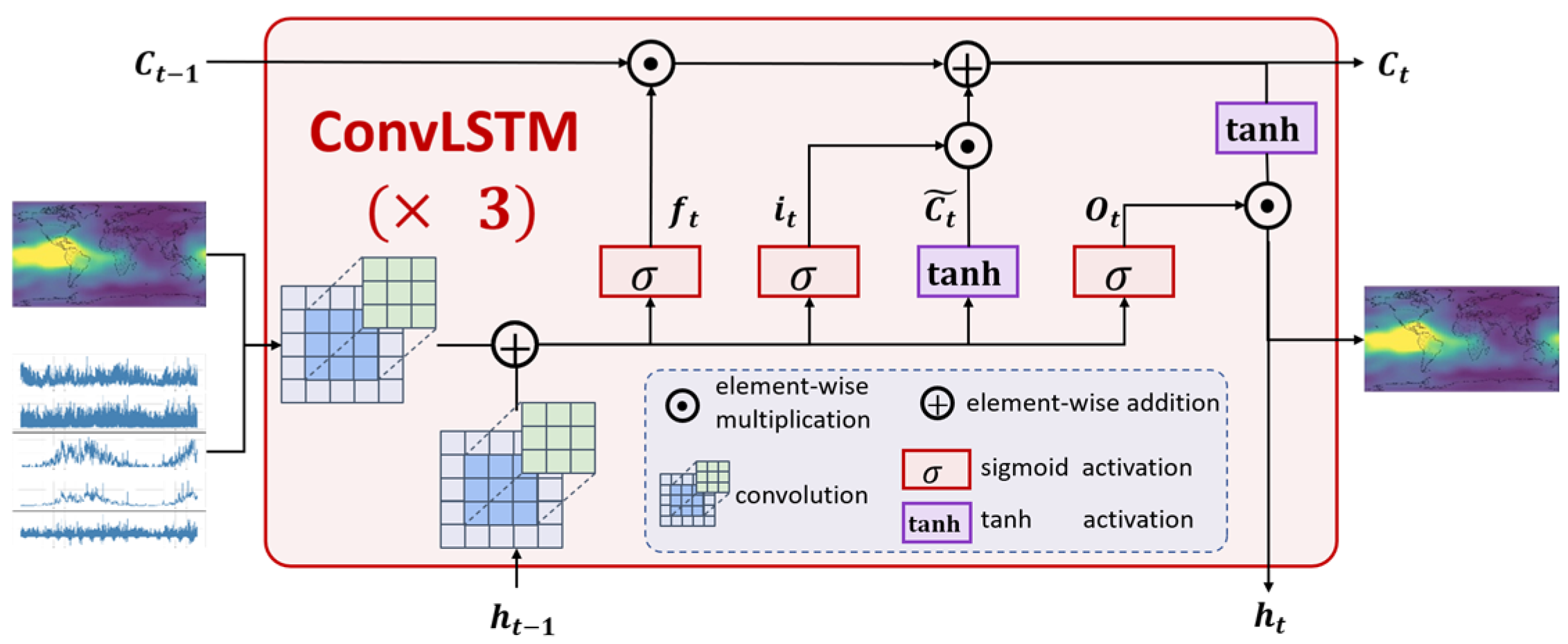
A stacked convolutional long short-term memory (ConvLSTM) network was adopted as the baseline model architecture for the present 24 h-ahead VTEC task. By combining the spatial feature extraction capability of convolutional neural networks (CNNs) with the temporal dependency modeling ability of long short-term memory (LSTM) networks, ConvLSTM is well suited to capturing the strongly coupled spatiotemporal evolution of VTEC. As shown in Figure 1, the proposed framework consists of three components: a stacked ConvLSTM encoder, an external-driver fusion layer, and an output projection layer. In the ConvLSTM cell shown in Figure 1, $H_t$ and $C_t$ denote the hidden state and cell state, respectively, $i_t$, $f_t$ and $o_t$ denote the input, forget, and output gates, and $\widetilde{C_t}$ denotes the candidate cell state. Here, $\sigma$ denotes the sigmoid activation function, which maps gate values to the range [0,1] and controls how much information is retained, updated, or output, whereas tanh denotes the hyperbolic tangent activation function, which maps values to [−1,1] and is used to generate the candidate state and regulate the hidden-state output.

The two-dimensional input to the ConvLSTM encoder consists of historical VTEC together with spatial encoding features and temporal encoding features. The input tensor is organized as (batch size, time steps, channels, height, width), corresponding to dimensions of (batch size, 24, 9, 71, 73). The nine channels include one VTEC feature channel, four spatial encoding channels, and four temporal encoding channels. It should be noted that the external drivers are not expanded into two-dimensional maps before entering the ConvLSTM encoder. Instead, they are retained as a one-dimensional auxiliary vector, projected into a latent representation, spatially broadcast to match the hidden feature-map size, and fused with the encoded TEC representation in the external-driver fusion layer.

The stacked ConvLSTM encoder comprises three sequential ConvLSTM layers with 32, 32, and 16 hidden channels, respectively. All layers use a kernel size of 3 × 3 and padding of 1 to preserve the spatial dimensions throughout the network. Through the coordinated action of the input, forget, and output gates, the network dynamically filters and propagates relevant spatiotemporal information, thereby learning complex VTEC evolution patterns.

To incorporate external forcing information, an external-driver fusion layer was introduced. The five-dimensional driver vector was first projected into a 16-dimensional latent representation through a fully connected layer. The resulting latent vector was then broadcast to match the spatial dimensions of the ConvLSTM output and concatenated with the extracted spatiotemporal features. This design allows solar and geomagnetic driver information to be integrated with the primary VTEC representation so that external forcing information can be incorporated into the final prediction process.

Finally, a 1 × 1 convolutional layer was used as the output projection layer to map the fused features to a 24-channel output corresponding to the predicted VTEC fields for the next 24 h. The output tensor has dimensions of (batch size, 24, 71, 73), ensuring that the predicted fields retain the same spatial resolution as the input data.

2.2.2. Training Strategy

The model was trained using the smooth L1 loss, which is less sensitive to outliers than the mean squared error and can improve training stability by reducing the influence of extreme samples. AdamW, an adaptive gradient optimizer with decoupled weight decay, was adopted as the optimizer, with an initial learning rate of 6 × 10^-4 and a weight decay coefficient of 1 × 10⁻⁵. Compared with the original Adam formulation with L2-style penalty, AdamW applies weight decay separately from the gradient-based parameter update, which helps improve generalization performance and stabilize training.

To avoid overfitting and unnecessary iterations, an early stopping strategy was applied with a patience of 10 epochs. Training was terminated when the decrease in validation loss remained smaller than 1 × 10⁻⁶ for 10 consecutive epochs, and the model parameters corresponding to the minimum validation loss were retained.

Mixed-precision training was employed to improve computational efficiency and reduce training time. To ensure reproducibility, the random seed was fixed at 42. The batch size was set to 128, the maximum number of training epochs was 100, and the gradient clipping threshold was fixed at 1.0 to maintain numerical stability during optimization.

2.2.3. Evaluation Metrics

Model performance was evaluated using three standard metrics: root mean square error (RMSE), mean absolute error (MAE), and coefficient of determination (R²). RMSE is defined as

$$\mathrm{RMSE}=\sqrt{{\displaystyle \frac{1}{N}}{\displaystyle \sum _{i=1}^N}{\left(y_i-\widehat{y_i}\right)}^2},$$

MAE is defined as

$$\mathrm{MAE}={\displaystyle \frac{1}{N}}{\displaystyle \sum _{i=1}^N}|y_i-\widehat{y_i}|,$$

and R² is defined as

$${\mathrm{R}}^2=1-{\displaystyle \frac{{\displaystyle {\sum }_{i=1}^N}{\left(y_i-\widehat{y_i}\right)}^2}{{\displaystyle {\sum }_{i=1}^N}{\left(y_i-\overline{y_i}\right)}^2}},$$

where $N$ denotes the total number of samples, $y_i$ denotes the observed VTEC value, $\widehat{y_i}$ denotes the predicted VTEC value, and $\overline{y_i}$ denotes the mean of the observed values. RMSE emphasizes larger errors, MAE reflects the average magnitude of the prediction error, and R² measures the proportion of variance explained by the model.

3. Results and Analysis

3.1. Overall Prediction Performance

Six comparative experiments were conducted to quantify the effects of different external drivers and their combinations on VTEC prediction performance. All models were built on the same stacked ConvLSTM framework, and performance was evaluated using RMSE, MAE, and R², whose definitions are given in Section 2.2.3.

As shown in

Table 1. Overall Prediction Performance Metrics of the Six Models on The Test Set.

	ConvLSTM	+All	+DST	+F10.7	+F10.7+DST	+DST+AU
RMSE	3.0626	3.0206	3.0622	3.1459	3.0294	3.0650
MAE	1.8309	1.8139	1.8326	1.8528	1.8128	1.8303
R2	0.9568	0.9579	0.9568	0.9544	0.9577	0.9567

Note: Bold values indicate the best performance in each row.

, the contribution of external drivers was not simply additive; instead, model performance depended strongly on the specific driver combination, indicating clear interaction and complementarity among the selected factors. Introducing F10.7 alone resulted in slightly poorer performance than the baseline model, suggesting that solar radiative information alone was insufficient to improve the representation of VTEC disturbances and may introduce additional uncertainty. By contrast, adding DST alone produced results close to those of the baseline, indicating that although DST is a physically meaningful driver, its individual contribution was insufficient to markedly improve overall model performance.

The combined use of F10.7 and DST yielded performance close to that of the full-factor model, implying that solar radiation and global geomagnetic forcing provide complementary information for characterizing the major coupled processes governing VTEC variability. In contrast, the DST+AU configuration remained close to the baseline, suggesting limited additional benefit because both variables represent geomagnetic activity and therefore contain partially overlapping information.

Among all configurations, the full-factor model (ConvLSTM+All) showed the most favorable overall average performance. By supplementing the core F10.7–DST coupling with additional information on solar wind dynamics (Vp) and composition (Na/Np), the full-factor model is better adapted to complex near-Earth forcing conditions and produced the lowest overall errors. It should also be noted that the R² values in Table 1 vary only within a narrow range (0.9544–0.9579). This indicates that all six models already explain most of the large-scale variance in the test set, so the global-average R² metric is relatively insensitive to the modest differences among driver configurations in this high-skill setting. For this reason, the practical comparison in this study relies more on RMSE, MAE, and condition-dependent analyses across disturbance levels, latitude bands, and lead times, rather than on the very small differences in global-average R² alone.

To assess whether deep learning is justified beyond simple temporal extrapolation, we further compared the ConvLSTM-based models with two classical statistical baselines, namely SARIMA and Holt–Winters exponential smoothing [38,39]. Under the same 24 h-ahead setting and the same chronological non-overlapping block partition, both statistical baselines performed clearly worse than the ConvLSTM-based models (

Table 2. Comparison between deep-learning models and classical statistical baselines on the test set.

	SARIMA	Holt-Winters	ConvLSTM	ConvLSTM+All
RMSE	5.6386	5.0546	3.0626	3.0206
MAE	2.8559	2.9582	1.8309	1.8139
R2	0.8534	0.8822	0.9568	0.9579

Note: Bold values indicate the best performance in each row.

). Specifically, the SARIMA baseline yielded a MAE of 2.856 TECU, an RMSE of 5.639 TECU, and an R² of 0.853, whereas the Holt–Winters baseline yielded a MAE of 2.958 TECU, an RMSE of 5.055 TECU, and an R² of 0.882. By comparison, the baseline ConvLSTM achieved a MAE of 1.831 TECU, an RMSE of 3.063 TECU, and an R² of 0.957, while the full-factor ConvLSTM+All further improved the results to a MAE of 1.814 TECU, an RMSE of 3.021 TECU, and an R² of 0.958. These comparisons suggest that, in the present global 24 h-ahead prediction setting, deep learning is justified relative to simple statistical forecasting baselines, while the selected external drivers provide further gains on top of the ConvLSTM backbone.

3.2. Performance Under Different Geomagnetic Disturbance Levels

To evaluate model adaptability under different ionospheric states, the test samples were divided into four disturbance levels according to the DST index: Quiet (DST > −30 nT), Minor (−30 ≥ DST > −50 nT), Moderate (−50 ≥ DST > −100 nT), and Severe (DST ≤ −100 nT). The corresponding results are summarized in

Table 3. RMSE and MAE (TECU) of the six models under different geomagnetic disturbance levels. For each entry, the first number denotes RMSE and the second denotes MAE.

level	ConvLSTM	+F10.7	+DST	+F10.7+DST	+DST+AU	+All
Quiet	2.72/1.65	2.80/1.67	2.71/1.65	2.69/1.63	2.73/1.65	2.68/1.63
Minor	3.62/2.32	3.71/2.35	3.71/2.37	3.65/2.33	3.70/2.35	3.65/2.34
Moderate	5.05/3.23	5.19/3.30	5.12/3.26	5.01/3.20	4.99/3.19	4.91/3.16
Severe	7.23/4.79	7.22/4.80	6.87/4.57	6.85/4.58	6.85/4.52	6.94/4.61

Note: Bold values indicate the best performance in each row.

.

Prediction errors increased systematically with disturbance intensity. From Quiet to Severe conditions, both RMSE and MAE rose across all model configurations, indicating that stronger geomagnetic forcing substantially increases the difficulty of 24 h-ahead global VTEC prediction. This overall pattern confirms that disturbed ionospheric states remain a major source of uncertainty for all tested models.

The usefulness of external drivers was clearly disturbance-dependent. Under Quiet conditions, the multi-factor configurations showed the most favorable performance. In particular, the full-factor model achieved the lowest RMSE, whereas the ConvLSTM+F10.7+DST configuration yielded the lowest MAE, suggesting that under relatively stable ionospheric conditions, the integration of multiple external drivers can provide modest but measurable benefits.

Under Minor disturbance conditions, however, the baseline ConvLSTM remained the best-performing configuration. All driver-augmented variants produced slightly larger errors than the baseline, indicating that additional external information does not necessarily translate into improved prediction when the ionosphere is only weakly disturbed. This result further suggests that, in such cases, the contribution of external drivers may be limited relative to the predictive information already contained in the historical VTEC sequence itself.

The benefit of external drivers became more evident under Moderate conditions. In this regime, the full-factor model provided the best overall performance, with both RMSE and MAE lower than those of the baseline and the other competing configurations. By contrast, the ConvLSTM+F10.7 model remained consistently worse than the baseline, implying that solar radiative information alone is insufficient to capture the dominant processes governing disturbed VTEC variability. These results indicate that once the ionosphere departs more clearly from quiet background conditions, a coordinated combination of solar, geomagnetic, and solar wind-related information becomes more useful than single-factor forcing.

Under Severe disturbance conditions, the advantage shifted toward DST-centered and geomagnetic-dominant combinations. The ConvLSTM+F10.7+DST configuration achieved the lowest RMSE, while the ConvLSTM+DST+AU configuration yielded the lowest MAE. The full-factor model also improved upon the baseline, but it no longer represented the best-performing configuration in this category. This pattern suggests that, under strong geomagnetic forcing, indices more directly associated with storm-time magnetospheric and auroral activity are more informative than F10.7 alone and may even be more effective than a broader multi-factor combination.

Overall, the results in Table 3 indicate that the optimal driver configuration is not fixed across all geomagnetic conditions. Instead, its effectiveness depends strongly on disturbance intensity. Multi-source forcing is more beneficial under Quiet and Moderate conditions, whereas under Severe disturbance, the most useful information is concentrated in geomagnetic-driver combinations dominated by DST and AU.

3.3. Spatial Characteristics of Prediction Errors

Figure 2 and Figure 3 present grid-wise error statistics aggregated over the full test set rather than prediction results from a specific day. For each grid cell, RMSE and MAE were computed by aggregating all available 24 h-ahead predictions in the test subset. The baseline map provides the overall error background, whereas the subtraction maps highlight where each driver configuration improves or degrades prediction relative to the baseline. Positive values indicate error reduction, whereas negative values indicate error increase. Although the large-scale background patterns remain visually similar across models, this is expected because all configurations share the same ConvLSTM backbone and are evaluated on the same test set. The purpose of the subtraction maps is to reveal the relatively subtle but spatially coherent differences in error reduction and error increase that are not easily distinguishable from the absolute maps alone.

The subtraction maps reveal clear differences among the driver configurations. The ConvLSTM+F10.7 model shows predominantly negative $\Delta \mathit{RMSE}$ and $\Delta \mathit{MAE}$ values across broad low-latitude belts, indicating that F10.7 alone does not consistently improve the baseline model and may even degrade performance in parts of the equatorial region. By contrast, the ConvLSTM+DST model shows more positive differences in several low-latitude and middle-to-high-latitude sectors, suggesting that geomagnetic forcing is more effective in reducing baseline errors, although the benefit remains geographically heterogeneous.

The pronounced low-latitude bands in Figure 2 and Figure 3 are broadly consistent with the equatorial ionization anomaly (EIA) region [40]. The EIA is one of the most prominent structures in the low-latitude ionosphere and is characterized by a trough near the magnetic equator and enhanced TEC crests on both sides, together with strong meridional gradients and marked longitudinal variability. These features increase the difficulty of global gridded prediction and help explain why the clearest spatial differences among models are concentrated in the equatorial belt. In this sense, the low-latitude error pattern should not be interpreted merely as a generic equatorial background effect, but more specifically as a model sensitivity to EIA-related structure and variability [41,42].

Relative to the baseline, the multi-factor configurations, especially ConvLSTM+DST+AU and ConvLSTM+All, show broader positive $\Delta \mathit{RMSE}$ and $\Delta \mathit{MAE}$ regions and a weaker concentration of negative differences in several low-latitude and auroral sectors. This suggests that combining multiple external drivers can partially mitigate EIA- and geomagnetic-related error patterns, although the improvement remains spatially nonuniform.

Table 4. RMSE, MAE, and R² of the six models in three magnetic-latitude zones.

		ConvLSTM	+F10.7	+DST	+F10.7+DST	+DST+AU	+All
Low magnetic latitude	RMSE	4.3583	4.5391	4.4099	4.3453	4.4071	4.3347
	MAE	2.7291	2.8046	2.7615	2.7199	2.7607	2.7249
	R2	0.9524	0.9484	0.9513	0.9527	0.9513	0.9529
Middle magnetic latitude	RMSE	2.6281	2.6514	2.5748	2.5619	2.5654	2.5578
	MAE	1.5523	1.5592	1.5383	1.5280	1.5296	1.5295
	R2	0.9371	0.9360	0.9396	0.9402	0.9401	0.9404
High magnetic latitude	RMSE	2.2762	2.2817	2.2586	2.2457	2.2849	2.2330
	MAE	1.3619	1.3617	1.3596	1.3461	1.3638	1.3442
	R2	0.8992	0.8987	0.9007	0.9019	0.8984	0.9030

Note: Three geomagnetic latitude zones are defined based on absolute magnetic latitude: low (0–30°), middle (30–60°), and high (60–90°). Bold values indicate the best performance in each row.In middle magnetic latitudes, the benefit of external drivers becomes more evident. Relative to the baseline, the ConvLSTM+DST, ConvLSTM+F10.7+DST, ConvLSTM+DST+AU, and ConvLSTM+All models all reduced RMSE and MAE, indicating that geomagnetic forcing contributes more clearly to improved predictive consistency in this latitude band. The corresponding R² values also increased slightly, but the differences remained small. Among the tested configurations, the full-factor model achieved the lowest RMSE (2.5578 TECU), while the ConvLSTM+F10.7+DST model yielded the lowest MAE (1.5280 TECU). Overall, the practical improvement in this latitude band is better reflected by error reduction than by the very small differences in R² alone.

summarizes the RMSE, MAE, and R² of the six models in low-, middle-, and high-magnetic-latitude zones. The tabulated results further confirm that the utility of external drivers is strongly latitude-dependent. In low magnetic latitudes, the differences among model configurations remain relatively modest. Although the full-factor model achieved the lowest RMSE (4.3347 TECU), the overall gain over the baseline remained limited. The corresponding R² differences were also very small, suggesting that the dominant errors in this region are closely related to EIA-associated structure and strong low-latitude gradients.

In high magnetic latitudes, the contribution of external drivers is even clearer. Relative to the baseline, DST-based and multi-factor configurations all reduced error and improved goodness of fit, reflecting the stronger sensitivity of high-latitude ionospheric variability to geomagnetic forcing. The full-factor model again showed the most favorable overall performance, with the lowest RMSE (2.2330 TECU), the lowest MAE (1.3442 TECU), and the highest R² (0.9030). These results indicate that geomagnetic drivers and multi-source forcing information are more beneficial in middle and high magnetic latitudes, whereas the gain remains more limited in low magnetic latitudes because of the greater structural complexity of EIA-related errors.

Taken together, the latitude-zone metrics summarized in Table 4 indicate that the contribution of external drivers is strongly latitude-dependent. In middle and high magnetic latitudes, geomagnetic drivers contribute more clearly to improved predictive consistency. In low magnetic latitudes, however, the gain remains more limited because the dominant errors are concentrated in EIA-related regions characterized by strong TEC gradients and greater structural complexity.

3.4. Error Patterns During a Geomagnetic Storm Event

Figure 4 provides an illustrative example of model behavior during the geomagnetic storm event on 17 March 2015 from 19:00 to 23:00 UT. Although all models show broadly similar large-scale error polarity, the baseline ConvLSTM configuration exhibits the largest error amplitude, especially in high latitudes. The ConvLSTM+F10.7 model shows only limited improvement, whereas DST-based and multi-factor configurations reduce the storm-time error amplitude more clearly. In this sense, the event-scale behavior is consistent with the broader conclusion from Table 3 that geomagnetic drivers are more useful than F10.7 alone under disturbed conditions.

3.5. Lead-Time-Dependent Prediction Performance

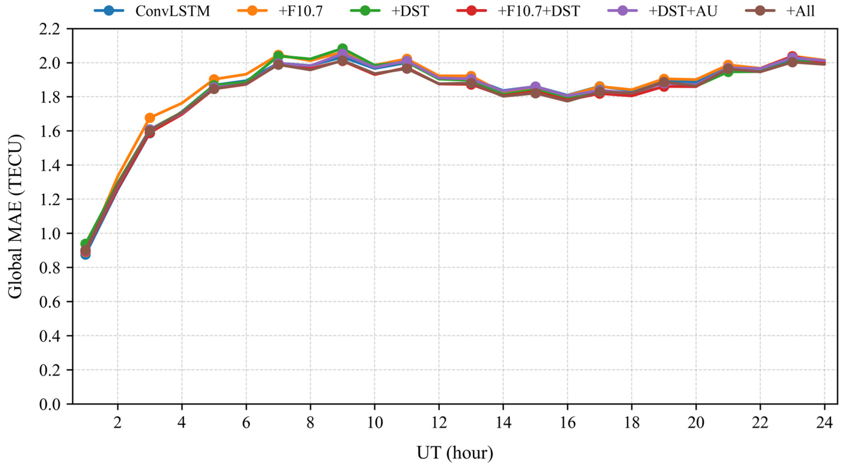
Figure 5 presents the temporal evolution of global MAE for all six models over the 24 h prediction horizon. For all models, MAE increased with lead time, reflecting the natural accumulation of error over longer prediction horizons. At the beginning of the prediction period, the MAE values of all models were close, ranging from approximately 0.8 to 0.9 TECU. Although some differences became visible after the early lead-time stages, the curves remained relatively close over much of the 24 h horizon.

The baseline ConvLSTM model showed the fastest growth in error, with MAE reaching approximately 1.9 TECU by 6 h. By contrast, the models incorporating geomagnetic drivers, particularly ConvLSTM+DST, ConvLSTM+DST+AU, and ConvLSTM+All, tended to show slower error growth during some middle and later lead times. Among them, the full-factor model maintained relatively low MAE over most of the prediction period. Overall, Figure 5 suggests a tendency toward improved long-horizon stability rather than a large and uniform improvement at every prediction step. Given that the external drivers are introduced as auxiliary variables at the forecast start and then fused with the encoded TEC representation, this behavior is more plausibly interpreted as improved sensitivity to the disturbance state at initialization, which then helps reduce subsequent error propagation, rather than as an explicit time-varying long-term constraint throughout the full 24 h horizon.

4. Discussion

The results indicate that the contribution of external drivers to deep learning-based VTEC prediction depends not only on whether additional variables are introduced, but also on how these variables are selected and combined. This finding highlights the importance of balancing statistical contribution, redundancy control, and physical interpretability when incorporating solar and geomagnetic information into data-driven prediction models. In this study, the proposed four-step feature selection strategy identified five core drivers, namely F10.7, DST, AU, Vp, and Na/Np, which jointly represent solar radiation, geomagnetic disturbance, solar wind dynamics, and particle composition. Within the present experimental setting, the overall results suggest that a physically coordinated driver set may be more useful than either a single-factor input or a less systematically selected combination.

A notable result is that the predictive gain associated with external drivers was strongly scenario-dependent. Under relatively quiet geomagnetic conditions, the full-factor configuration achieved the best performance, indicating that the regular evolution of VTEC can benefit from the integration of multi-source background information. In contrast, under severe disturbance conditions, the best-performing configurations shifted toward combinations dominated by geomagnetic indices, especially DST and AU. This pattern suggests that, under severe disturbance, the dominant source of prediction uncertainty is no longer only the background ionospheric state, but also the abrupt forcing associated with geomagnetic activity. In this context, geomagnetic indicators provide more direct and timely information than solar radiative indices alone. This interpretation is also consistent with the physical role of F10.7, which primarily characterizes the background level of solar radiation rather than the short-term intensity and structure of geomagnetic forcing.

The results also reveal pronounced latitudinal dependence in the effectiveness of external drivers. At low magnetic latitudes, the gain from external drivers remained limited, but this should not be interpreted simply as a lack of low-latitude variability. Rather, the dominant errors in this region are closely related to EIA-associated structure, which is characterized by strong TEC gradients and pronounced longitudinal variability. These features make low-latitude prediction intrinsically difficult and help explain why the improvement pattern remains spatially heterogeneous even when external drivers are introduced. By contrast, in middle and especially high latitudes, geomagnetic drivers produced larger improvements. This regional contrast is consistent with the stronger sensitivity of middle- and high-latitude ionospheric variability to geomagnetic forcing. In particular, the reductions in high-latitude error under DST-, AU-, and full-factor configurations indicate that geomagnetic information is important for constraining disturbance-driven deviations that are difficult to learn from VTEC history alone. The broader positive ΔRMSE and ΔMAE regions shown by the multi-factor configurations further suggest that multi-source driver fusion may help reduce the concentration of EIA- and geomagnetic-related error patterns, although the improvement remains spatially nonuniform.

Another important finding is that the inclusion of external drivers affected not only overall predictive performance but also prediction stability over time. The slower MAE growth observed in the full-factor and geomagnetic-driver models suggests that appropriate driver selection may help limit error accumulation over a 24 h prediction horizon. In the present architecture, however, the external drivers are introduced as an auxiliary vector at the forecast start and fused with the encoded TEC representation, rather than being supplied as a time-varying future forcing sequence. Therefore, the reduced error growth is more reasonably interpreted as a consequence of improved sensitivity to the initial disturbance state and better conditioning of the forecast initialization. This effect then propagates through the multi-step prediction, rather than acting as a continuous long-term external constraint over the full lead-time window. This interpretation is also consistent with the stronger benefit of geomagnetic drivers under disturbed conditions, where accurate representation of the initial forcing state is especially important for reducing subsequent error propagation.

Although the selected driver configurations improved predictive performance under several conditions, the global-average gains remained modest. Therefore, the practical significance of the present findings should not be understood as a large universal improvement in operational accuracy, but rather as empirical evidence that the utility of external drivers is condition-dependent and that physically guided driver selection may be beneficial in specific settings.

From a methodological perspective, the proposed feature selection strategy provides a practical procedure for incorporating physical knowledge into deep learning-based ionospheric prediction within the present ConvLSTM-based setting and dataset configuration. Rather than relying solely on statistical importance or subjective experience, the strategy combines importance screening, redundancy removal, physical interpretability, and performance validation in a progressive manner. This helps avoid two common problems in driver construction: the omission of physically meaningful variables and the inclusion of redundant inputs that may degrade performance. The fact that the selected driver set achieved the best overall results suggests that careful driver selection is an important component of model design in this type of data-driven VTEC prediction setting, rather than a secondary preprocessing step. In addition, the comparison with SARIMA and Holt–Winters shows that the ConvLSTM-based framework remains advantageous relative to simple classical statistical forecasting baselines under the same prediction setting.

Several limitations should nevertheless be acknowledged. First, although the selected drivers improved predictive performance under most conditions, the gain remained limited under the most extreme storm scenarios, especially in high-latitude regions where error peaks were still evident. This suggests that the current model and driver set do not fully capture the rapid and highly nonlinear ionospheric response during severe geomagnetic events. Second, the present analysis was conducted using data from 2014 to 2018, and the relative utility of different drivers may vary across solar cycles or under different long-term background conditions. More importantly, the proposed feature selection strategy was validated only within a single ConvLSTM-based architecture in the present study. Its transferability to other deep learning backbones, as well as to empirical or statistical prediction frameworks, therefore, remains unverified. Third, although the selected drivers span multiple physical processes, the model architecture itself remains data-driven and does not explicitly encode ionospheric physical constraints, which may limit physically grounded interpretation under highly disturbed conditions.

Future work may proceed in two directions. One is to improve high-latitude prediction under extreme geomagnetic storms by incorporating region-specific observations or disturbance-sensitive auxiliary data, thereby strengthening model responsiveness to abrupt auroral and polar ionospheric variability. The other is to examine whether the utility of external drivers varies across different solar cycle phases and, if so, whether such variation is large enough to justify a dynamic driver-selection mechanism under changing space-weather conditions. Such efforts may further improve the reliability and transferability of deep learning-based VTEC prediction under complex and extreme ionospheric environments.

5. Conclusions

This study examined how solar and geomagnetic driver selection affects 24 h-ahead global VTEC prediction within a ConvLSTM framework and proposed a four-step strategy for constructing a compact external-driver set. Among the tested combinations, the full-factor configuration showed the best overall performance, although its global-average improvement over the baseline remained modest. The results further indicate that the utility of external drivers is condition-dependent rather than universally additive, with clearer differences across geomagnetic disturbance levels, latitude bands, and prediction lead times. Overall, this study provides empirical support for more systematic and physically informed driver selection in data-driven VTEC prediction. The generality of this finding across other model architectures, time periods, and solar cycle conditions still requires further verification.

References

1. Blackband, W.T.; Burgess, B.; Jones, I.L.; Lawson, G.J. Deduction of ionospheric electron content from the Faraday fading of signals from artificial Earth satellites. Nature 1959, 183, 1172–1174. [Google Scholar] [CrossRef] [Scilit]
2. Breitsch, B.; Morton, Y.T.; Rino, C.; Carrano, C.; Xu, D. GNSS carrier phase cycle slips due to diffractive ionosphere scintillation: Simulation and characterization. IEEE Trans. Aerosp. Electron. Syst. 2020, 56, 3632–3644. [Google Scholar] [CrossRef] [Scilit]
3. Zhou, W.; Yuan, Y.; Tang, C.; Meng, Y.; Chen, Y. Ionosphere disturbances on GNSS signal and positioning performance: Analysis of the solar flare and geomagnetic storm events in September 2017 and October 2021. Adv. Space Res. 2024, 73, 4608–4620. [Google Scholar] [CrossRef] [Scilit]
4. Schmölter, E.; Berdermann, J. The impact of the 2024 Mother’s day storm on aircraft surveillance across Europe. Space Weather 2025, 23, e2025SW004718. [Google Scholar] [CrossRef] [Scilit]
5. Fang, T.-W.; Fuller-Rowell, T.; Yudin, V.; Matsuo, T.; Viereck, R. Quantifying the sources of ionosphere day-to-day variability. J. Geophys. Res. Space Phys. 2018, 123, 9682–9697. [Google Scholar] [CrossRef] [Scilit]
6. Guerra, M.; Cesaroni, C.; Fiorentino, N.; Tosone, F.; Ventriglia, V.; Pica, E.; Astafyeva, E.; Maletckii, B.; Spogli, L. Automatic detection of large-scale traveling ionospheric disturbances using GNSS data and image processing techniques. Space Weather 2025, 23, e2025SW004423. [Google Scholar] [CrossRef] [Scilit]
7. Ogwala, A.; Somoye, E.O.; Ogunmodimu, O.; Adeniji-Adele, R.A.; Onori, E.O.; Oyedokun, O. Diurnal, seasonal and solar cycle variation in total electron content and comparison with the IRI-2016 model at Birnin Kebbi. Ann. Geophys. 2019, 37, 775–789. [Google Scholar] [CrossRef] [Scilit]
8. Astafyeva, E.; Maletckii, B.; Förster, M.; Ouar, I.D.; Huba, J.D.; Hairston, M.R.; Coley, W.R. Electrodynamic and ionospheric puzzles of the 10–11 May 2024 geomagnetic superstorm. J. Geophys. Res. Space Phys. 2025, 130, e2024JA033284. [Google Scholar] [CrossRef] [Scilit]
9. Zakharenkova, I.; Cherniak, I.; Braun, J.J.; Weiss, J.P.; Wu, Q.; VanHove, T.; Hunt, D.; Sleziak-Sallee, M. Unveiling ionospheric response to the May 2024 superstorm with low-earth-orbit satellite observations. Space Weather 2025, 23, e2024SW004245. [Google Scholar] [CrossRef] [Scilit]
10. Zhen, W.M.; Ou, M.; Zhu, Q.L.; Dong, X.; Liu, D. Review on ionospheric sounding and modeling. Chin. J. Radio Sci. 2023, 38, 625–645. [Google Scholar] [CrossRef]
11. Cai, Y.; Yue, X.; Wang, W.; Zhang, S.-R.; Liu, H.; Lin, D.; Wu, H.; Yue, J.; Bruinsma, S.L.; Ding, F.; et al. Altitude extension of the NCAR-TIEGCM (TIEGCM-X) and evaluation. Space Weather 2022, 20, e2022SW003227. [Google Scholar] [CrossRef] [Scilit]
12. Themens, D.R.; Reid, B.; Jayachandran, P.T.; Larson, B.; Koustov, A.V.; Elvidge, S.; McCaffrey, A.M.; Watson, C. E-CHAIM as a model of total electron content: Performance and diagnostics. Space Weather 2021, 19, e2021SW002872. [Google Scholar] [CrossRef] [Scilit]
13. Bilitza, D.; Pezzopane, M.; Truhlik, V.; Altadill, D.; Reinisch, B.W.; Pignalberi, A. The International Reference Ionosphere model: A review and description of an ionospheric benchmark. Rev. Geophys. 2022, 60, e2022RG000792. [Google Scholar] [CrossRef] [Scilit]
14. Kim, J.-H.; Kwak, Y.-S. Validating the IRI-2020 model for ionospheric storms over the North-east Asian sector induced by extreme geomagnetic storms. Adv. Space Res. 2025, 75, 4347–4369. [Google Scholar] [CrossRef] [Scilit]
15. Schaer, S. Mapping and Predicting the Earth’s Ionosphere Using the Global Positioning System; Geodätisch-Geophysikalische Arbeiten in der Schweiz, Vol. 59; Institut für Geodäsie und Photogrammetrie, ETH Zürich: Zürich, Switzerland, 1999. [Google Scholar]
16. Jakowski, N.; Mayer, C.; Hoque, M.M.; Wilken, V. Total electron content models and their use in ionosphere monitoring. Radio Sci. 2011, 46, RS0D18. [Google Scholar] [CrossRef] [Scilit]
17. Materassi, M.; Alberti, T.; Migoya-Orué, Y.; Radicella, S.M.; Consolini, G. Chaos and predictability in ionospheric time series. Entropy 2023, 25, 368. [Google Scholar] [CrossRef] [Scilit]
18. Tang, J.; Ding, M.; Yang, D.; Fan, C.; Khonsari, N.; Mao, W. Different data-driven prediction of global ionospheric TEC using deep learning methods. Int. J. Appl. Earth Obs. Geoinf. 2024, 130, 103889. [Google Scholar] [CrossRef] [Scilit]
19. Zewdie, G.K.; Valladares, C.; Cohen, M.B.; Lary, D.J.; Ramanl, D.; Tsidu, G.M. Data-driven forecasting of low-latitude ionospheric total electron content using long short-term memory deep recurrent neural networks. Space Weather 2021, 19, e2020SW002639. [Google Scholar] [CrossRef] [Scilit]
20. Chen, J.; Zhi, N.; Liao, H.; Lu, M.; Feng, S. Global forecasting of ionospheric vertical total electron contents via ConvLSTM with spectrum analysis. GPS Solut. 2022, 26, 69. [Google Scholar] [CrossRef] [Scilit]
21. Yang, J.; Huang, W.; Xia, G.; Zhou, C.; Chen, Y. Operational forecasting of global ionospheric TEC maps 1-, 2-, and 3-day in advance by ConvLSTM model. Remote Sens. 2024, 16, 1700. [Google Scholar] [CrossRef] [Scilit]
22. Shih, C.-Y.; Lin, C.Y.-T.; Lin, S.-Y.; Yeh, C.-H.; Huang, Y.-M.; Hwang, F.-N.; Chang, C.-H. Forecasting of global ionosphere maps with multi-day lead time using transformer-based neural networks. Space Weather 2024, 22, e2023SW003579. [Google Scholar] [CrossRef] [Scilit]
23. Lin, Y.; Fang, H.; Duan, D.; Huang, H.; Xiao, C.; Ren, G. Enhanced forecasting of global ionospheric vertical total electron content maps using deep learning methods. Atmosphere 2024, 15, 1319. [Google Scholar] [CrossRef] [Scilit]
24. Ren, X.; Yang, P.; Liu, H.; Chen, J.; Liu, W. Deep learning for global ionospheric TEC forecasting: Different approaches and validation. Space Weather 2022, 20, e2021SW003011. [Google Scholar] [CrossRef] [Scilit]
25. Mao, S.; Pan, Y.; Kłopotek, G.; Schartner, M.; Krásná, H.; de Witt, A.; Soja, B. Enhanced global ionospheric mapping using deep ensemble neural networks with uncertainty quantification. Space Weather 2025, 23, e2025SW004446. [Google Scholar] [CrossRef] [Scilit]
26. Adolfs, M.; Hoque, M.M.; Shprits, Y.Y. Storm-time relative total electron content modelling using machine learning techniques. Remote Sens. 2022, 14, 6155. [Google Scholar] [CrossRef] [Scilit]
27. Feng, J.; Zhang, Y.; Li, W.; Han, B.; Zhao, Z.; Zhang, T.; Huang, R. Analysis of ionospheric TEC response to solar and geomagnetic activities at different solar activity stages. Adv. Space Res. 2023, 71, 2225–2239. [Google Scholar] [CrossRef] [Scilit]
28. Kim, J.-H.; Kwak, Y.-S.; Kim, Y.H.; Moon, S.-I.; Jeong, S.-H.; Yun, J. Potential of regional ionosphere prediction using a long short-term memory deep-learning algorithm specialized for geomagnetic storm period. Space Weather 2021, 19, e2021SW002741. [Google Scholar] [CrossRef] [Scilit]
29. Han, B.; Yu, Q.; Wang, J.; Chernogor, L.F.; Zheng, Y. An ionospheric VTEC forecasting model over China based on the kernel ridge regression. Adv. Space Res. 2025, 76, 353–370. [Google Scholar] [CrossRef] [Scilit]
30. Ren, X.; Yang, P.; Mei, D.; Liu, H.; Xu, G.; Dong, Y. Global ionospheric TEC forecasting for geomagnetic storm time using a deep learning-based multi-model ensemble method. Space Weather 2023, 21, e2022SW003231. [Google Scholar] [CrossRef] [Scilit]
31. Wang, S.; Huang, S. Quantify the information contributions of external drivers to ionospheric TEC variability. J. Geophys. Res. Space Phys. 2023, 128, e2023JA031897. [Google Scholar] [CrossRef] [Scilit]
32. Chen, Z.; Liao, W.; Li, H.; Wang, J.; Deng, X.; Hong, S. Prediction of global ionospheric TEC based on deep learning. Space Weather 2022, 20, e2021SW002854. [Google Scholar] [CrossRef] [Scilit]
33. Ren, X.; Zhao, B.; Ren, Z.; Wang, Y.; Xiong, B. Deep learning-based prediction of global ionospheric TEC during storm periods: Mixed CNN-BiLSTM method. Space Weather 2024, 22, e2024SW003877. [Google Scholar] [CrossRef] [Scilit]
34. Chen, J.; Xiong, P.; Wu, H.; Zhang, X.; Zhang, X.; Chai, R.; Zhang, T.; Wang, K.; Wang, C. High-precision prediction of ionospheric TEC in the China region based on CMONOC high-resolution data and an auxiliary attention temporal convolutional network. J. Geophys. Res. Mach. Learn. Comput. 2025, 2, e2025JH000608. [Google Scholar] [CrossRef] [Scilit]
35. Luo, H.; Gong, Y.; Chen, S.; Yu, C.; Yang, G.; Yu, F.; Hu, Z.; Tian, X. Prediction of global ionospheric total electron content (TEC) based on SAM-ConvLSTM model. Space Weather 2023, 21, e2023SW003707. [Google Scholar] [CrossRef] [Scilit]
36. Viall, N.M.; Borovsky, J.E. Nine outstanding questions of solar wind physics. J. Geophys. Res. Space Phys. 2020, 125, e2018JA026005. [Google Scholar] [CrossRef] [Scilit]
37. Kepko, L.; Viall, N.M.; DiMatteo, S. Periodic mesoscale density structures comprise a significant fraction of the solar wind and are formed at the sun. J. Geophys. Res. Space Phys. 2024, 129, e2023JA031403. [Google Scholar] [CrossRef] [Scilit]
38. Hill, P.; Biggs, J.; Ponce-López, V.; Bull, D. Time-series prediction approaches to forecasting deformation in Sentinel-1 INSAR data. J. Geophys. Res. Solid Earth 2021, 126, e2020JB020176. [Google Scholar] [CrossRef] [Scilit]
39. Chatfield, C. The Holt-winters forecasting procedure. J. R. Stat. Soc. Ser. C (Appl. Stat.) 1978, 27, 264–279. [Google Scholar] [CrossRef] [Scilit]
40. Nigussie, M.; Jakowski, N.; Hoque, M. Characterization and climatological modeling of equatorial ionization anomaly (EIA) crest position. J. Geophys. Res. Space Phys. 2022, 127, e2022JA030798. [Google Scholar] [CrossRef] [Scilit]
41. Mukhtarov, P.; Pancheva, D.; Andonov, B.; Pashova, L. Global TEC maps based on GNSS data: 1. Empirical background TEC model. J. Geophys. Res. Space Phys. 2013, 118, 4594–4608. [Google Scholar] [CrossRef] [Scilit]
42. Balan, N.; Liu, L.B.; Le, H.J. A brief review of equatorial ionization anomaly and ionospheric irregularities. Earth Planet. Phys. 2018, 2, 257–275. [Google Scholar] [CrossRef] [Scilit]
Figure 1. Overall architecture of the ConvLSTM model. The TEC sequence is represented as a two-dimensional grid map, whereas the external drivers are treated as one-dimensional auxiliary variables. These auxiliary variables are not expanded into two-dimensional maps before entering the ConvLSTM encoder; instead, they are fused with the encoded TEC representation after linear projection and spatial broadcasting.
Geosciences 16 00169 g001
Figure 2. Baseline RMSE distribution and baseline-referenced RMSE differences for the five driver-augmented models, computed by aggregating all 24 h-ahead predictions over the full test set. The upper-left panel shows the absolute RMSE of the baseline ConvLSTM model. The remaining panels show Δ RMSE =   RMSE baseline   RMSE model , where positive values indicate lower error than the baseline model and negative values indicate higher error. These panels are intended to highlight the spatial improvement or degradation associated with each driver configuration.
Geosciences 16 00169 g002
Figure 3. Baseline MAE distribution and baseline-referenced MAE differences for the five driver-augmented models, computed by aggregating all 24 h-ahead predictions over the full test set. The upper-left panel shows the absolute MAE of the baseline ConvLSTM model. The remaining panels show Δ MAE = MAE baseline   MAE model , where positive values indicate lower error than the baseline model and negative values indicate higher error. These panels are intended to highlight the spatial improvement or degradation associated with each driver configuration.
Geosciences 16 00169 g003
Figure 4. Illustrative storm-case prediction-error maps for the six models during the geomagnetic storm on 17 March 2015 (19:00–23:00 UT). Prediction error is defined as predicted VTEC minus observed VTEC. Positive values indicate overestimation, whereas negative values indicate underestimation. This figure is intended as a qualitative event-scale complement to the aggregated analyses presented in the main text.
Geosciences 16 00169 g004
Figure 5. Temporal Evolution of Global MAE for Six Models over the 24 h Prediction Horizon.
Geosciences 16 00169 g005